Covariant generalization of cosmological perturbation theory

Abstract

We present an approach to cosmological perturbations based on a covariant perturbative expansion between two worldlines in the real inhomogeneous universe. As an application, at an arbitrary order we define an exact scalar quantity which describes the inhomogeneities in the number of e-folds on uniform density hypersurfaces and which is conserved on all scales for a barotropic ideal fluid. We derive a compact form for its conservation equation at all orders and assign it a simple physical interpretation. To make a comparison with the standard perturbation theory, we develop a method to construct gauge-invariant quantities in a coordinate system at arbitrary order, which we apply to derive the form of the $n$-th order perturbation in the number of e-folds on uniform density hypersurfaces and its exact evolution equation. On large scales, this provides the gauge-invariant expression for the curvature perturbation on uniform density hypersurfaces and its evolution equation at any order.

I Introduction

Relativistic perturbation theory is an extremely useful tool for studying primordial inhomogeneities in cosmology and interpreting cosmological data such as the Cosmic Microwave Background (CMB) temperature anisotropies. The linear perturbation theory has been developed to a very high degree of sophistication Lifshitz:1963ps ; Bardeen:1980kt ; Kodama:1985bj ; Mukhanov:1990me and due to the smallness of the CMB temperature fluctuations usually provides an excellent approximation of the evolution of cosmological inhomogeneities. However, in order to reliably compare the theory with the high accuracy of the present and future observations, it has become important to study perturbations beyond the linear order, and recently there has been a flourishing activity around this subject. The foundation of second and higher order perturbation theory has been given in Bruni ; secondorder , although already at second order the coordinate approach becomes computationally challenging (see for example Bartolo ; Noh:2004bc ; Nakamura ).

Instead of resorting to higher orders, one can alternatively use non-perturbative methods to study the nonlinear evolution of cosmological perturbations. Most of these methods Salopek:1990jq ; Comer:1994np ; Sasaki:1998ug ; Lyth:2003im ; Rigopoulos:2003ak ; proof are based on the so-called long wavelength approximation, which restricts their validity to super-Hubble scales.

A non-perturbative and covariant way to deal with relativistic inhomogeneities has been proposed by Ellis and Bruni Ellis:1989jt and thereafter employed mainly in its linearized version to study cosmological perturbations as an alternative to the coordinate approach Bruni:1992dg . There one defines perturbations of scalar quantities as covectors that vanish in a spatially homogenous and isotropic Friedmann-Lemaître-Robertson-Walker (FLRW) universe. The advantage of the covariant formalism is that it directly deals with geometrical quantities that are not hampered by the gauge problems of the standard perturbation theory.

Recently, the covariant formalism was revived in Langlois:2005ii ; Langlois:2006iq ; Langlois:2006vv as a convenient way to derive exact equations describing the nonlinear evolution of perturbations, without resorting to any approximations. In Langlois:2005ii it was shown that, for a barotropic ideal fluid, it is possible to define a covector which is conserved exactly and on all scales in the Lie derivation along the fluid flow.

The existence of a conserved quantity in cosmology is of paramount importance as it allows one to establish a connection between perturbations at different epochs without solving for the detailed evolution of the universe. The result of Langlois:2005ii generalizes the approximate large-scale conservation of the so-called curvature perturbation on uniform density hypersurfaces in perturbation theory. This quantity was introduced in linear theory in Bardeen:1980kt ; Bardeen , rederived using the continuity equation alone in Hwang:1991aj ; Wands:2000dp and extended to second order in the perturbations in Malik:2003mv . Nonlinear generalizations for the curvature perturbation have also been derived using the long wavelength approximation in Lyth:2003im ; Rigopoulos:2003ak ; proof .

In the present paper, we present a covariant approach for the study of nonlinear perturbations and their conservation properties based on a perturbative expansion similar to the standard coordinate-based perturbation theory. However, in the coordinate approach a perturbation is defined as the difference between the values that a quantity (a scalar or a tensor) takes in the real inhomogeneous universe and in a fictitious ideal background, whereas in our approach a perturbation is defined geometrically in the real inhomogeneous universe as the difference between the values of a quantity measured by two observers on different worldlines. Thus, the terms in our covariant expansion are tensors in the real universe, not coordinate-based perturbations around an ideal homogeneous universe. Our definition also implies that the perturbation of a tensor of a given type is described by a tensor of the same type. Thus, in contrast to the approach of Ellis:1989jt , the perturbations of scalar fields are described by scalars and not by covectors.

As in the standard coordinate approach, our perturbative expansion allows us to write a hierarchy of equations which, order by order, are coupled with those of lower order. However, being covariantly defined in the real universe, our quantities are automatically gauge-independent, thus avoiding the complications of the gauge issue of the standard perturbation theory.

To demonstrate the efficiency of our approach, we apply it to the continuity equation of an ideal fluid. At each order in covariant perturbations, we define a scalar quantity $\zeta_{(n)}$ which generalizes, on large scales, the curvature perturbation on uniform density hypersurfaces at the same order. We derive an exact evolution equation for $\zeta_{(n)}$, showing that at arbitrary order it is conserved for a barotropic ideal fluid. This equation manifestly mimics the perturbative large-scale evolution equation of the curvature perturbation on uniform density hypersurfaces.

This paper is organized as follows. In Sec. II we briefly review the covariant formalism for nonlinear cosmological perturbations. In Sec. III we define our covariant perturbative expansion and apply it to the continuity equation. Section IV is devoted to the comparison between our covariant perturbative expansion with the standard coordinate-based approach. Finally, in Sec. V we draw our conclusions.

II Covariant formalism

In this section we briefly review the basic ideas of the covariant approach to perturbations proposed in Ellis:1989jt and recently used to study the conservation and evolution of nonlinear relativistic perturbations for a perfect fluid Langlois:2005ii , for dissipative interacting fluids Langlois:2006iq and for scalar fields Langlois:2006vv .

We consider a universe dominated by an ideal fluid characterized by a four-velocity $u^{a}=dx^{a}/d\tau$ ($u_{a}u^{a}=-1$), where $\tau$ is the proper time of an observer comoving with the fluid. The energy-momentum tensor of the fluid is

$$T^{a}_{\ b}=\rho u^{a}u_{b}+ph^{a}_{\ b},$$ (1)

where $h^{a}_{\ b}$ is the spatial projection tensor orthogonal to the four-velocity $u^{a}$,

$$h_{ab}\equiv g_{ab}+u_{a}u_{b},\quad\quad(h^{a}_{\ c}h^{c}_{\ b}=h^{a}_{\ b},\quad h^{a}_{\ b}u^{b}=0).$$ (2)

In the covariant approach, the deviations from a spatially homogeneous and isotropic FLRW universe are described by tensor fields defined in the real inhomogeneous universe and vanishing in an FLRW spacetime. The inhomogeneities of scalar quantities that do not vanish in the background can be described in a simple way by considering the spatial projections of their covariant derivatives Ellis:1989jt . For any scalar $f$ one can define the projected gradient

$$D_{a}f\equiv h_{a}^{\ b}\nabla_{b}f,$$ (3)

which vanishes in the FLRW background and is thus interpreted as a perturbation. This definition is purely geometrical and depends only on the four-velocity $u^{a}$. Since the covector $D_{a}f$ is defined in the real inhomogeneous universe, it can be conveniently employed to describe nonlinear perturbations without having to rely on a perturbative expansion around an ideal homogeneous background.

In Langlois:2005ii , the covariant approach was used to define conserved nonlinear perturbations from the continuity equation, obtained by contracting the conservation equation of the energy-momentum tensor,

$$\nabla_{b}T^{b}_{\ a}=0,$$ (4)

with the fluid four-velocity $u^{a}$. For an ideal fluid, the continuity equation reads

$$\dot{\rho}+3\dot{\alpha}(\rho+p)=0,$$ (5)

where $\alpha$ is the local number of e-folds defined as the integral of the volume expansion along a worldline,

$$\alpha\equiv\frac{1}{3}\int\nabla_{a}u^{a}d\tau,\qquad(3\dot{\alpha}=\nabla_{a}u^{a}),$$ (6)

and the dot denotes the covariant derivative projected along $u^{a}$,

$$\dot{\alpha}\equiv\nabla_{u}\alpha.$$ (7)

Here, for convenience, we have adopted the short notation

$$\nabla_{v}\equiv v^{a}\nabla_{a}$$ (8)

for the covariant derivative along a generic vector $v^{a}$, that we shall use hereafter. We remind here also the expression for the Lie derivative along a vector $v^{a}$, which will be useful in the following. For a scalar quantity $f$, this is equivalent to the covariant derivative along $v^{a}$, i.e.,

$${\cal L}_{v}f=\nabla_{v}f.$$ (9)

For a vector $w^{a}$ it is equivalent to the commutator between $v^{a}$ and $w^{a}$,

$${\cal L}_{v}w^{a}=[v,w]^{a}\equiv\nabla_{v}w^{a}-\nabla_{w}v^{a},$$ (10)

while for a covector $w_{a}$ it is given by

$${\cal L}_{v}w_{a}=\nabla_{v}w_{a}+w_{b}\nabla_{a}v^{b}.$$ (11)

In order to “extract” an evolution equation for covariant perturbations from Eq. (5), one can simply take the spatially projected gradient $D_{a}$ of this equation and invert the time derivative and the spatial gradient. One can define a covector Langlois:2005ii ,

$$\zeta_{a}\equiv D_{a}\alpha-\frac{\dot{\alpha}}{\dot{\rho}}D_{a}\rho,$$ (12)

that satisfies a remarkably simple conservation equation in the Lie derivative along $u^{a}$,

$${\cal L}_{u}\zeta_{a}=\frac{3\dot{\alpha}^{2}}{\dot{\rho}}\left(D_{a}p-\frac{\dot{p}}{\dot{\rho}}D_{a}\rho\right).$$ (13)

Equation (13) is fully nonlinear and exact on all scales. For a barotropic fluid, i.e., when the pressure of the fluid is a unique local function of the energy density, $p=p(\rho)$, its right hand side vanishes and $\zeta_{a}$ is exactly conserved under Lie derivation along the worldlines of comoving observers. When expanded to first order in the standard perturbation theory, $\zeta_{a}$ reduces on large scales to the spatial gradient of the first-order curvature perturbation on uniform density hypersurfaces, usually denoted by $\zeta$. Furthermore, on large scales Eq. (13) mimics the evolution equation of $\zeta$.

III Covariant perturbation theory

III.1 Covariant perturbations

Here we define a covariant perturbative expansion in the real inhomogeneous universe, which allows us to introduce the concept of $n$-th order covariant perturbations. We first consider the perturbations of a scalar quantity $f$. Later, we will generalize our definitions to a tensor field.

In an inhomogeneous universe, two comoving observers living on different worldlines and measuring the same proper time $\tau$ will in general observe different values of $f$ whereas in an FLRW universe they would measure the same (homogeneous) value. Thus, one can describe the inhomogeneities of $f$ by considering the difference between the values of $f$ measured by two neighboring comoving observers.

To characterize the separation between these observers, we introduce a connecting vector $e^{a}\equiv dx^{a}/d\lambda$ that commutes with the fluid four-velocity ellis ,

$$[u,e]^{a}=0,\qquad(\Leftrightarrow\quad{\cal L}_{u}e^{a}=0).$$ (14)

As shown in Fig. 1, for each value of the proper time $\tau$, the connecting vector $e^{a}$ defines an integral curve, parameterized by $\lambda$, linking observers that measure the same proper time. These observers define a continuous family of worldlines and Eq. (14) guarantees that the parameters $\tau,\lambda$ can be used as (timelike and spacelike, respectively) coordinates on this two-dimensional hypersurface.

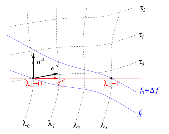
Figure 1: Geometric definition of the covariant perturbation $\Delta f_{\lambda_{\perp}}$

on the two-dimensional hypersurface with the coordinates $\{\tau,\lambda\}$.

The connecting vector $e^{a}$ is not, in general, orthogonal to the fluid four-velocity $u^{a}$, but can be decomposed into a longitudinal part, parallel to $u^{a}$, and a relative position vector $e_{\perp}^{a}$, orthogonal to $u^{a}$ ellis , as

$$e^{a}\equiv e^{a}_{\perp}+e_{\parallel}u^{a},\qquad(e_{\perp}^{a}=h^{a}_{\ b}e^{b},~{}e_{||}=-u^{a}e_{a}).$$ (15)

The relative position vector $e_{\perp}^{a}$ defines another integral curve, parameterized by $\lambda_{\perp}$, which characterizes the separation between neighboring observers as measured in their rest frame.

We now define the perturbation of $f$ by comparing the values measured by observers on the integral curve of $e_{\perp}^{a}$. For convenience, we choose the parametrization of the curve such that these observers are at $\lambda_{\perp}=0$ and $\lambda_{\perp}=1$, respectively:

$$\Delta f\equiv f(1)-f(0).$$ (16)

This can be taylor-expanded along the integral curve of $e_{\perp}^{a}$ as,

$$\Delta f=\sum_{n=1}^{\infty}\frac{1}{n!}\left.\nabla_{e_{\perp}}^{n}f\right|_{0},$$ (17)

where $\left.\right|_{0}$ denotes the restriction to $\lambda_{\perp}=0$. Each term in the expansion (17) vanishes in the FLRW background and thus we define the $n$-th order term in Eq. (17) as the $n$-th order covariant perturbation of $f$.

The first-order term of the expansion (17), i.e., the covariant first-order perturbation ${\nabla_{e_{\perp}}}f$, has actually been introduced already in the appendix of Ellis:1989jt as a scalar analogue of the spatially projected gradient $D_{a}f$ employed in the standard covariant approach. Indeed, it can be written as

$$\nabla_{e_{\perp}}f=e^{a}D_{a}f.$$ (18)

In contrast, the higher order covariant perturbations in (17) have not been discussed previously in the literature.

The definition of the covariant $n$-th order perturbation of a scalar can be easily generalized to an arbitrary tensor field $T$ living in the inhomogeneous real spacetime, which we denote by ${\cal M}$, by defining a diffeomorphism between $\lambda_{\perp}=0$ and $\lambda_{\perp}=1$. This can be accomplished by using the flow $\Phi:\mathbb{R}\times{\cal M}\to{\cal M}$, generated by the vector field $e_{\perp}^{a}$. The diffeomorphism $\Phi$ defines a pullback $\Phi^{*}_{\lambda_{\perp}}$ which maps a tensor $T$ at $\lambda_{\perp}$ into a tensor $\Phi^{*}_{\lambda_{\perp}}T$ at $\lambda_{\perp}=0$. The perturbation of the tensor field $T$ can then be defined as

$$\Delta T\equiv\Phi^{*}_{1}\left.T\right|_{0}-\left.T\right|_{0}.$$ (19)

In an FLRW universe any tensor field $T$ is invariant under $\Phi^{*}_{\lambda_{\perp}}$ because this corresponds to a transformation of the coordinates on the homogeneous spatial hypersurfaces. Therefore $\Delta T$ describes a perturbation around the FLRW background and, as in the scalar case, it can be taylor-expanded as

$$\Delta T=\sum_{n=1}^{\infty}\frac{1}{n!}\left.{\cal L}_{e_{\perp}}^{n}T\right|_{0}.$$ (20)

The n-th order term ${\cal L}_{e_{\perp}}^{n}\left.T\right|_{0}$ in this expansion is the $n$-th order covariant perturbation of the tensor field $T$. If $T$ is a scalar field, the Lie derivative is just the directional derivative and we recover the expression (17).

The perturbation (19) and the perturbative expansion (20) have been defined here in analogy to the standard coordinate-based perturbation theory Bruni . However, instead of living in an ideal background spacetime, $\Delta T$ and each term in its expansion are geometrically defined quantities in the real inhomogeneous universe. The $n$-th order covariant perturbations ${\cal L}^{n}_{e_{\perp}}T$ measure how the tensor field $T$ changes in the direction of $e_{\perp}^{a}$. Therefore they depend on the choice of $e_{\perp}^{a}$ but this is not a source of ambiquity since $e_{\perp}^{a}$ is a vector field in the real universe and can be given a physical meaning.

III.2 Evolution of perturbations

Now we study the evolution of perturbations employing our covariant perturbative expansion for scalar quantities and applying it to the continuity equation. Using this perturbative expansion we expand the continuity equation (5) and define at each order a quantity that is exactly conserved along the fluid flow for adiabatic (isentropic) perturbations, i.e., if the ideal fluid is barotropic.

We begin by considering the evolution of covariant first-order perturbations. By applying the spatial derivative $\nabla_{e_{\perp}}$ to Eq. (5) we find

$$\nabla_{e_{\perp}}\dot{\rho}+3(\rho+p)\nabla_{e_{\perp}}\dot{\alpha}+3\dot{\alpha}(\nabla_{e_{\perp}}\rho+\nabla_{e_{\perp}}p)=0.$$ (21)

Now we want to invert the time derivative with the space derivative along $e^{a}_{\perp}$. However, before doing so we note that $e^{a}_{\perp}$ does not, in general, commute with $u^{a}$ but one has

$$[u,e_{\perp}]^{a}=-\dot{e}_{\parallel}u^{a}$$ (22)

which implies that

$$\nabla_{e_{\perp}}\dot{f}={{(\nabla_{e_{\perp}}f)}^{\hbox{.}}}+\dot{e}_{\parallel}\dot{f}.$$ (23)

Using this relation and Eq. (5), we can rewrite Eq. (21) as

$${{\left(\nabla_{e_{\perp}}\alpha-\frac{\dot{\alpha}}{\dot{\rho}}\nabla_{e_{\perp}}\rho\right)}^{\hbox{.}}}=\frac{3\dot{\alpha}^{2}}{\dot{\rho}}\left(\nabla_{e_{\perp}}p-\frac{\dot{p}}{\dot{\rho}}\nabla_{e_{\perp}}\rho\right),$$ (24)

which has the same form as Eq. (13) but is written in terms of scalar quantities instead of covectors. Indeed, this equation can be also found by projecting Eq. (13) along $e^{a}$, and making use of Eqs. (14) and (18).

It is convenient to re-express Eq. (24) by defining the vector field

$${\tilde{e}}^{a}\equiv e_{\perp}^{a}-\frac{\nabla_{e_{\perp}}\rho}{\dot{\rho}}u^{a}=e^{a}-\frac{\nabla_{e}\rho}{\dot{\rho}}u^{a}$$ (25)

(the second equality follows from Eq. (15)), which lies on a uniform density hypersurface, as one can check by contracting its definition with $\nabla_{a}\rho$. Using this vector, Eq. (24) can be rewritten as

$${{\left(\nabla_{{\tilde{e}}}\alpha\right)}^{\hbox{.}}}=\frac{3\dot{\alpha}^{2}}{\dot{\rho}}\nabla_{{\tilde{e}}}p.$$ (26)

Note that although in Eq. (24) we have used covariant derivatives along the spatially projected vector $e_{\perp}^{a}$ to define the perturbations, because of the second equality of Eq. (25) one can replace these by covariant derivatives along $e^{a}$.

The quantity

$$\nabla_{\tilde{e}}\alpha=\nabla_{e}\alpha-\frac{\nabla_{e}\rho}{\dot{\rho}}\dot{\alpha},\qquad(\nabla_{\tilde{e}}\rho=0),$$ (27)

describes the change of $\alpha$ when going from a worldline to a neighboring one along the integral curve of $e^{a}$ projected on uniform density hypersurfaces. This can be seen more clearly by rewriting the previous expression in terms of the coordinates $\{\tau,\lambda\}$, which yields

$$\nabla_{\tilde{e}}\alpha=\frac{d\alpha}{d\lambda}-\frac{\dot{\alpha}}{\dot{\rho}}\frac{d\rho}{d\lambda}=\left.\frac{\partial\alpha}{\partial\lambda}\right|_{\rho},$$ (28)

where the second equality follows from the change of variables $\{\tau,\lambda\}\to\{\rho,\lambda\}$. Thus, $\nabla_{\tilde{e}}\alpha$ in Eq. (26) is the covariant first-order perturbation of the integrated expansion $\alpha$ on uniform density hypersurfaces and $\nabla_{\tilde{e}}p$ is the covariant first-order non-adiabatic pressure perturbation.

By introducing the notation

$$\zeta_{(1)}\equiv\nabla_{\tilde{e}}\alpha,$$ (29)

and

$$\Gamma_{(1)}\equiv\nabla_{\tilde{e}}p,$$ (30)

the evolution equation (26) can be written as

$$\dot{\zeta}_{(1)}=\frac{3\dot{\alpha}^{2}}{\dot{\rho}}\Gamma_{(1)},$$ (31)

which shows that $\zeta_{(1)}$ is conserved if $\Gamma_{(1)}=0$. This equation is exact and fully nonlinear and generalizes the large-scale first-order conservation equation of the curvature perturbation on uniform density hypersurfaces $\zeta$.

From Eq. (28) we can interpret the conservation of $\zeta_{(1)}$ for a barotropic fluid as follows (see also the discussion of Lyth:2003im ; proof ). The continuity equation of an ideal fluid, Eq. (5), can be integrated along each comoving worldline yielding

$$\alpha=-\int\frac{d\rho}{3(\rho+p)},\qquad(\lambda={\rm const}).$$ (32)

If the fluid is barotropic, $p=p(\rho)$ is the same function for all worldlines, and Eq. (32) can be explicitly integrated yielding

$$\alpha=\tilde{\alpha}(\rho)+c(\lambda),$$ (33)

where $\tilde{\alpha}(\rho)$ is a function of $\rho$ and $c(\lambda)$ is an integration constant (along a worldline) that may change from a worldline to another, and reflects that $\alpha$ is defined up to a constant. Since $\nabla_{\tilde{e}}\tilde{\alpha}=0$, from Eqs. (29) and (28) this expression yields

$$\zeta_{(1)}=\left.\frac{\partial c}{\partial\lambda}\right|_{\rho},$$ (34)

which is constant along the fluid flow. However, if the fluid is non-barotropic, the equation of state $p=p(\rho,\lambda)$ may vary from a worldline to another implying that the dependence of $\alpha$ on $\rho$ also changes and $\zeta_{(1)}$, as defined in Eq. (28), is no longer conserved.

Before extending our analysis to an arbitrary order, we first consider covariant second-order perturbations for which we know the coordinate-based perturbative analogue. As explained above, in our covariant approach the operator $\nabla_{e_{\perp}}$ is used to define perturbations and $\nabla_{{\tilde{e}}}$ combines these to construct perturbations on uniform density hypersurfaces. In order to find the second-order perturbed evolution equation we can apply once more $\nabla_{e_{\perp}}$ to Eq. (21). However, it is more convenient to expand the continuity equation in perturbations on uniform density hypersurfaces, applying directly $\nabla_{{\tilde{e}}}$ to Eq. (26). Using the commutation relation

$$[{\tilde{e}},u]^{a}={{\left(\frac{\nabla_{e}\rho}{{\dot{\rho}}}\right)}^{\hbox{.}}}u^{a},$$ (35)

which follows from the definition of ${\tilde{e}}^{a}$ and implies

$$\nabla_{\tilde{e}}\dot{f}={{(\nabla_{\tilde{e}}f)}^{\hbox{.}}}+{{\left(e_{\parallel}+\frac{\nabla_{e_{\perp}}\rho}{\dot{\rho}}\right)}^{\hbox{.}}}\dot{f},$$ (36)

we find a second-order evolution equation,

$$\dot{\zeta}_{(2)}=\frac{3\dot{\alpha}^{2}}{\dot{\rho}}\Gamma_{(2)}+\frac{6\dot{\alpha}}{\dot{\rho}}\dot{\zeta}_{(1)}\Gamma_{(1)},$$ (37)

where we have defined the covariant second-order perturbation of $\alpha$ on uniform density hypersurfaces as

$$\zeta_{(2)}\equiv\nabla_{\tilde{e}}^{2}\alpha,$$ (38)

and the covariant second-order non-adiabatic pressure perturbation as

$$\Gamma_{(2)}\equiv\nabla_{\tilde{e}}^{2}p.$$ (39)

Expanding the definition (38) in terms of spatial perturbations one obtains

$$\zeta_{(2)}=\nabla_{e_{\perp}}^{2}\alpha-\frac{\dot{\alpha}}{\dot{\rho}}\nabla_{e_{\perp}}^{2}\rho-\frac{2}{\dot{\rho}}\nabla_{e_{\perp}}\rho\left[{{(\nabla_{e_{\perp}}\alpha)}^{\hbox{.}}}-\frac{\dot{\alpha}}{\dot{\rho}}{{(\nabla_{e_{\perp}}\rho)}^{\hbox{.}}}\right]+\frac{1}{\dot{\rho}}{{\left(\frac{\dot{\alpha}}{\dot{\rho}}\right)}^{\hbox{.}}}(\nabla_{e_{\perp}}\rho)^{2},$$ (40)

and the explicit expansion of $\Gamma_{(2)}$ can be read from Eq. (40) by replacing $\alpha$ by $p$.

Equation (37) is the evolution equation for $\zeta_{(2)}$. It implies that $\zeta_{(2)}$ is conserved on all scales if the first and second-order non-adiabatic pressure perturbations vanish, i.e., $\Gamma_{(1)}=\Gamma_{(2)}=0$. The form of Eq. (40) and the evolution equation (37) mimic and generalize the large-scale result of the second-order coordinate approach Malik:2003mv .

We are now ready to extend our analysis to arbitrary order by defining the covariant $n$-th order perturbation of $\alpha$ on uniform density hypersurfaces as

$$\zeta_{(n)}\equiv\nabla_{\tilde{e}}^{n}\alpha=\left(\nabla_{e}-\frac{\nabla_{e}\rho}{\dot{\rho}}\nabla_{u}\right)^{n}\alpha,$$ (41)

and the $n$-th order non-adiabatic pressure perturbation as

$$\Gamma_{(n)}\equiv\nabla_{\tilde{e}}^{n}p.$$ (42)

To find the evolution equation of $\zeta_{(n)}$, one can apply the operator $\nabla_{\tilde{e}}^{n}$ to the continuity equation (5) and recursively use the commutation relation (36) and $\nabla_{\tilde{e}}\rho=0$ to invert the time and space derivatives. After a series of straightforward manipulations one obtains

$$\dot{\zeta}_{(n)}=\frac{3}{\dot{\rho}}\sum_{l=0}^{n-1}\sum_{m=0}^{n-l-1}\frac{(n-1)!}{l!m!(n-l-m-1)!}\dot{\zeta}_{(n-l-m-1)}\dot{\zeta}_{(m)}\Gamma_{(l+1)},$$ (43)

where we have defined

$$\zeta_{(0)}\equiv\alpha.$$ (44)

For any order of the perturbative expansion defined in Sec. III.1, this evolution equation shows that $\zeta_{(n)}$ is conserved on all scales if the fluctuations are adiabatic up to this order, i.e., $\Gamma_{(k)}=0,~{}k=1,\ldots,n$. Indeed, for a barotropic fluid, Eq. (33) implies that $\zeta_{(n)}$ is conserved along a worldline at all orders. The definition of $\zeta_{(n)}$ Eq. (41) and its evolution equation (43) are among our main results.

IV Comparison with the coordinate-based approach

Most of the studies of inhomogeneities in cosmology have been done in the coordinate-based perturbation theory. Thus, it is important to establish a connection between our covariant perturbations and the quantities used in the coordinate approach.

In this section we construct at arbitrary order in the coordinate-based perturbation theory the expression and evolution equation of the perturbation of the integrated expansion on uniform density hypersurfaces, which on large scales coincides with the curvature perturbation on uniform density hypersurfaces, thus extending the previously known first and second-order results. Then, we explicitly expand the covariant variable $\zeta_{(n)}$ given in Eq. (41) in terms of perturbations in a coordinate system and show that, in the uniform energy density gauge, it reduces on large scales to the spatial gradient of the $n$-th order uniform density curvature perturbation.

IV.1 Perturbation theory and gauge transformations

In the standard coordinate-based perturbation theory (see e.g. Nakamura ; Bruni ) one considers a $5$-dimensional manifold $\mathcal{N}=\mathcal{M}\times\mathbb{R}$, each $\mathcal{M}$ being labelled by the continuous parameter $y$. Each submanifold $\mathcal{M}_{y}$, together with the tensor fields $T_{y}$ living on it, describes a spacetime model which interpolates between an ideal FLRW background, at $y=0$, and the real inhomogeneous universe, at $y=1$. The real universe can then be described approximately by an expansion in the parameter $y$ around the background solution. In the following we choose the parameter $y$ to be the fifth coordinate on $\mathcal{N}$, $x^{4}=y$, and use capital indices $A,B$ running from $0$ to $4$ to denote the components of a tensor field on $\mathcal{N}$.

To define the perturbation of a tensor field $T$ around the background spacetime $y=0$, one needs a map between the submanifolds $\mathcal{M}_{y}$, which can be constructed as the flow ${\cal X}_{y}:\mathcal{M}_{0}\rightarrow\mathcal{M}_{y}$ of a vector field $X^{A}$ defined on $\cal N$ such that $X^{4}=1$ everywhere. Thus, $X^{A}$ is always transverse to ${\cal M}_{y}$ and connects different leaves of the foliation of $\cal N$. The perturbation of a tensor field $T$ can then be defined as Bruni

$$(\Delta_{X}T)_{y}\equiv{\cal X}^{*}_{y}\left.T\right|_{0}-\left.T\right|_{0},$$ (45)

where the subscript $0$ denotes the restriction to the background spacetime $\mathcal{M}_{0}$ and we recall that ${\cal X}^{*}_{y}T$ is the pull-back of $T_{y}$. This can be taylor-expanded in the parameter $y$ as

$$(\Delta_{X}T)_{y}=\sum_{n=1}^{\infty}\frac{y^{n}}{n!}\left.{\cal L}_{X}^{n}T\right|_{0},$$ (46)

and the $n$-th order term of this expansion defines the $n$-th order perturbation of $T$,

$$\delta_{X}^{n}T\equiv{\cal L}_{X}^{n}\left.T\right|_{0}.$$ (47)

The definitions of the perturbation of $T$ and of its perturbative expansion depend on the choice of the vector field $X^{A}$, or equivalently of the diffeomorphism ${\cal X}_{y}$. This is commonly referred to as the choice of gauge and therefore Eq. (47) defines the $n$-th order perturbation of $T$ in the gauge $X^{A}$. Instead of $X^{A}$, one can define the perturbation of $T$ by using another vector field $Y^{A}$ with $Y^{4}=1$,

$$(\Delta_{Y}T)_{y}\equiv{\cal Y}^{*}_{y}\left.T\right|_{0}-\left.T\right|_{0},$$ (48)

where ${\cal Y}_{y}$ is the flow generated by $Y^{A}$. One can expand this equation similarly to Eq. (46) and define the $n$-th order perturbation of $T$ in the gauge $Y^{A}$ as

$$\delta_{Y}^{n}T\equiv\left.{\cal L}_{Y}^{n}T\right|_{0}.$$ (49)

The transformation from the gauge $X^{A}$ to $Y^{A}$ is generated by the diffeomorphism $({\cal Y}_{-y}\circ{\cal X}_{y}):\mathcal{M}_{0}\to\mathcal{M}_{0}$. One can taylor-expand its action on $(\Delta_{y}T)_{X}$ and explicitly work out how the perturbations transform order by order, defining at each order a generator of the gauge transformation as a vector field living on the background spacetime Bruni . For our purposes, it is more convenient to express the gauge transformation in terms of the vector field $\xi^{A}$ defined as

$$\xi^{A}\equiv Y^{A}-X^{A},$$ (50)

which will be called here the total generator of the gauge-transformation to distinguish it from the generators defined order by order. Equation (50) defines $\xi^{A}$ for each value of $y$ and can therefore be used to generate gauge transformations at arbitrary order. Note that $\xi^{4}$ vanishes identically due to the choice $X^{4}=Y^{4}=1$ showing that $\xi^{A}$ evaluated for a given $y$ is always tangent to ${\cal M}_{y}$.

The $n$-th order perturbation of a tensor field $T$ in the gauge $Y^{A}$ can now be written in terms of the perturbations in the gauge $X^{A}$ and the total generator $\xi^{A}$ as

$$\delta_{Y}^{n}T=\left.{\cal L}^{n}_{Y}T\right|_{0}=\left.({\cal L}_{X}+{\cal L}_{\xi})^{n}T\right|_{0}.$$ (51)

One can employ this compact formula to derive the gauge-invariant expression of the perturbation of $T$ in the gauge $Y^{A}$ at any order.

The gauge transformations derived from Eq. (51) are equivalent to those derived in Bruni . When expanding the right hand side of Eq. (51) to $n$-th order, one finds combinations of commutators of the vector fields $X^{A}$ and $\xi^{A}$ that are equivalent to the $n$ independent generators defined in Bruni . Indeed, this can be demonstrated up to third order by explicitly expanding Eq. (51). By employing the following useful expression for the commutator of two Lie derivatives along the vector fields $v^{A}$ and $w^{A}$,

$$[{\cal L}_{v},{\cal L}_{w}]={\cal L}_{[v,w]},$$ (52)

this yields

$$\delta_{Y}T = \delta_{X}T+{\cal L}_{\xi_{(1)}}\left.T\right|_{0},$$ (53)

$$\delta_{Y}^{2}T = \delta_{X}^{2}T+({\cal L}_{\xi_{(2)}}+{\cal L}^{2}_{\xi_{(1)}})\left.T\right|_{0}+2{\cal L}_{\xi_{(1)}}\delta_{X}T,$$ (54)

$$\delta_{Y}^{3}T = \delta_{X}^{3}T+({\cal L}_{\xi_{(3)}}+3{\cal L}_{\xi_{(1)}}{\cal L}_{\xi_{(2)}}+{\cal L}_{\xi_{(1)}}^{3})\left.T\right|_{0}+3({\cal L}_{\xi_{(2)}}+{\cal L}_{\xi_{(1)}}^{2})\delta_{X}T+3{\cal L}_{\xi_{(1)}}\delta_{X}^{2}T,$$ (55)

where we have defined the first three generators of the gauge transformations as

$$\xi^{A}_{(1)} \equiv \left.\xi^{A}\right|_{0}=\left.Y^{A}-X^{A}\right|_{0},$$ (57)

$$\xi^{A}_{(2)} \equiv \left.[X,\xi]^{A}\right|_{0}=\left.[X,Y]^{A}\right|_{0},$$ (58)

$$\xi^{A}_{(3)} \equiv \left.[X-\xi,[X,\xi]]^{A}\right|_{0}=\left.[2X-Y,[X,Y]]^{A}\right|_{0},$$ (59)

and we have used Eq. (50) to rewrite them in the second equalities in the familiar form in terms of $X^{A}$ and $Y^{A}$, given in Bruni .

IV.2 Evolution of perturbations

In this section we derive the gauge-invariant expression and the evolution equation of the perturbation of the integrated expansion (or number of e-folds) on uniform density hypersurfaces at arbitrary order using Eq. (51). We focus on this quantity, instead of the curvature perturbation on uniform density hypersurfaces, because it is the conserved quantity that naturally arises when expanding the continuity equation. However, on large scales, i.e., neglecting spatial gradients as well as vector and tensor perturbations, as in the so-called separate universe approach Sasaki:1998ug ; Rigopoulos:2003ak ; proof ; Langlois:2005ii , the curvature perturbation coincides with the perturbation in the integrated expansion. Therefore, on these scales the uniform density integrated expansion coincides with the uniform density curvature perturbation, allowing us to establish also for the latter an expression on large scales at arbitrary order.

In the following we choose coordinates on the background manifold $\mathcal{M}_{0}$ such that the FLRW metric reads

$$ds^{2}=-dt^{2}+a^{2}(t)\gamma_{ij}dx^{i}dx^{j},$$ (60)

where $\gamma_{ij}$ is the homogeneous spatial metric and the four-velocity of the fluid is

$$\bar{u}^{a}=(1,0,0,0).$$ (61)

The uniform energy density gauge is defined by requiring that the perturbations of the energy density vanish to all orders. This determines the temporal gauge, or time-slicing, and additional conditions are needed to fix the remaining three degrees of freedom that correspond to the spatial gauge or threading. In the following we denote by $Y^{A}$ the gauge with uniform energy density slicing and comoving threading and derive the gauge-invariant expression for the perturbations of $\alpha$ in this gauge.

The conditions defining the gauge $Y^{A}$ can be expressed as

$${\cal L}_{Y}\rho = 0,$$ (62)

$${\cal L}_{Y}u^{A} \propto u^{A}.$$ (63)

The first condition guarantees that the perturbations of the energy density vanish to all orders,

$$\delta_{Y}^{n}\rho=0,$$ (64)

and the second condition sets the perturbations of the spatial components of the fluid four-velocity to zero

$$\delta^{n}_{Y}u^{i}=0.$$ (65)

By substituting Eq. (50) into Eqs. (62) and (63), we derive a set of conditions on the total generator $\xi^{A}$ that define the gauge transformation between the gauge $Y^{A}$ and a generic gauge $X^{A}$. To simplify the analysis, we decompose $\xi^{A}$ into parts orthogonal and parallel to the four-velocity $u^{A}$ as

$$\xi^{A}=\xi_{\parallel}u^{A}+\xi_{\perp}^{A},\qquad(\xi_{\perp}^{A}=h^{A}_{\ B}\xi^{B},~{}\xi_{\parallel}=-u^{A}\xi_{A}).$$ (66)

Using the condition for uniform energy density slicing, Eq. (62), we can rewrite $\xi^{A}$ as

$$\xi^{A}=-\frac{{\cal L}_{X}\rho}{\dot{\rho}}u^{A}+\tilde{\xi}^{A},$$ (67)

where we have defined

$$\tilde{\xi}^{A}\equiv\xi^{A}_{\perp}-\frac{{\cal L}_{\xi_{\perp}}\rho}{\dot{\rho}}u^{A}.$$ (68)

Furthermore, the condition for comoving threading, Eq. (63), yields a condition on the Lie derivative of $\tilde{\xi}^{A}$ along $u^{A}$, i.e.,

$${\cal L}_{u}\tilde{\xi}^{A}-{\cal L}_{X}u^{A}\propto u^{A}.$$ (69)

The expression for $\xi^{A}$ (67) with the condition (69) involves only perturbations in the gauge $X^{A}$ and by substituting it into Eq. (51) we obtain the gauge-invariant expression for $\delta_{Y}^{n}\alpha$,

$$\delta^{n}\zeta\equiv\delta_{Y}^{n}\alpha=\left.\left({\cal L}_{X}-\frac{{\cal L}_{X}\rho}{\dot{\rho}}{\cal L}_{u}+{\cal L}_{\tilde{\xi}}\right)^{n}\alpha\right|_{0},$$ (70)

where we have defined $\delta^{n}\zeta$ as the gauge-invariant $n$-th order perturbation of the integrated expansion on uniform density hypersurfaces.

Using Eq. (70) one can straightforwardly rederive the familiar first and second-order expressions for $\delta\zeta$ and $\delta^{2}\zeta$ and even go to higher orders. At first order $n=1$, using the definition of perturbations (47), Eq. (70) yields

$$\delta\zeta=\delta_{X}\alpha-\frac{H}{\bar{\rho}^{\prime}}\delta_{X}\rho,$$ (71)

where $\bar{\rho}\equiv\left.\rho\right|_{0}$ is the background value of the energy density, $H\equiv a^{\prime}/a=\bar{\alpha}^{\prime}$ the background Hubble parameter and the prime ^′ denotes the derivative with respect to the time coordinate $t$. The vector $\tilde{\xi}^{A}$ specifying the threading does not appear in this expression because $\left.{\cal L}_{\tilde{\xi}}\alpha\right|_{0}=0$. On large scales, $\delta_{X}\alpha$ is equivalent to the first-order curvature perturbation and Eq. (71) coincides with the well-known gauge-invariant expression for the curvature perturbation on uniform density hypersurfaces.

At second order, $n=2$, by using Eq. (52) for the commutator of two Lie derivatives, Eq. (70) becomes

$$\delta^{2}\zeta=\left.\left[\left({\cal L}_{X}-\frac{{\cal L}_{X}\rho}{\dot{\rho}}{\cal L}_{u}\right)^{2}\alpha+2{\cal L}_{\tilde{\xi}}\left({\cal L}_{X}\alpha-\frac{{\cal L}_{X}\rho}{\dot{\rho}}\dot{\alpha}\right)+{\cal L}_{[X-({{\cal L}_{X}\rho}/{\dot{\rho}})u,\tilde{\xi}]}\alpha+{\cal L}_{\tilde{\xi}}^{2}\alpha\right]\right|_{0}.$$ (72)

The last two terms vanish on the background manifold as one can show by using ${\cal L}_{\tilde{\xi}}\rho=0$ and $\tilde{\xi}^{0}\left.\right|_{0}=0$, while the second term is simply $2{\cal L}_{\tilde{\xi}_{(1)}}\delta\zeta$. Furthermore, when commuting ${\cal L}_{u}$ and ${\cal L}_{X}$ in the first term on the right hand side of Eq. (72) using Eq. (52), one encounters terms proportional to the commutator $[X,u]^{A}$. These terms do not vanish but appear in such a combination that they cancel when evaluated on the background. After these manipulations one arrives at

$$\delta^{2}\zeta=\delta_{X}^{2}\alpha-\frac{H}{\bar{\rho}^{\prime}}\delta_{X}^{2}\rho-\frac{2}{\bar{\rho}^{\prime}}\delta_{X}\rho\left(\delta_{X}\alpha^{\prime}-\frac{H}{\bar{\rho}^{\prime}}\delta_{X}\rho^{\prime}\right)+\frac{1}{\bar{\rho}^{\prime}}\left(\frac{H}{\bar{\rho}^{\prime}}\right)^{\prime}\delta_{X}\rho^{2}+2{\tilde{\xi}}_{(1)}^{i}\partial_{i}\delta\zeta,$$ (73)

where

$${\tilde{\xi}}_{(1)}^{i}\equiv\left.{\tilde{\xi}}^{i}\right|_{0}$$ (74)

is the generator of the first-order spatial gauge transformation from the gauge $X^{A}-({\cal L}_{X}\rho/{\dot{\rho}})u^{A}$ to $Y^{A}$ and for convenience we adopt the notation $\delta_{X}\rho^{\prime}\equiv(\delta_{X}\rho)^{\prime}$.

The first-order generator ${\tilde{\xi}}_{(1)}^{i}$ can be expressed in terms of the perturbations of $u^{A}$ restricting the spatial components of Eq. (69) to the background manifold, which yields

$${\tilde{\xi}}_{(1)}^{i}{}^{\prime}=\delta_{X}u^{i}.$$ (75)

Without the last term on the right hand side, Eq. (73) is equivalent to the second-order perturbation of the integrated expansion on uniform density hypersurfaces defined in Langlois:2005ii . Here, in addition we were able to account also for the last term of Eq. (73) that was present in Malik:2003mv , coming from the choice of threading. On large scales $\delta^{2}\zeta$ coincides with the curvature perturbation on uniform density hypersurfaces defined by Malik and Wands. (More precisely, it coincides with $\zeta^{(2)}_{\rm MW}-\zeta^{(1)}_{\rm MW}{}^{2}$.)

One of the advantages of the compact expression (70) is that one can straightforwardly work out the explicit gauge-invariant expression for $\delta^{n}\zeta$ at arbitrary order. To demonstrate this we give the explicit gauge-invariant expression of the third order perturbations of the integrated expansion on uniform density hypersurfaces. This can be computed similarly to the second-order case and one finds

$$\delta^{3}\zeta = \delta_{X}^{3}\alpha-\frac{H}{\bar{\rho}^{\prime}}\delta_{X}^{3}\rho-\frac{3}{\bar{\rho}^{\prime}}\left({\delta_{X}\alpha}^{\prime}-\frac{H}{\bar{\rho}^{\prime}}{\delta_{X}\rho}^{\prime}\right)\left(\delta_{X}^{2}\rho-2\frac{\delta_{X}\rho{\delta_{X}\rho}^{\prime}}{\bar{\rho}^{\prime}}+\frac{\bar{\rho}^{\prime\prime}}{\bar{\rho}^{\prime}{}^{2}}{\delta_{X}\rho}^{2}\right)$$ (76)

$$-3\frac{\delta_{X}\rho}{\bar{\rho}^{\prime}}\left(\delta_{X}^{2}\alpha^{\prime}-\frac{H}{\bar{\rho}^{\prime}}{\delta_{X}^{2}\rho}^{\prime}\right)+3\frac{\delta_{X}\rho^{2}}{\bar{\rho}^{\prime}{}^{2}}\left(\delta_{X}\alpha^{\prime\prime}-\frac{H}{\bar{\rho}^{\prime}}\delta_{X}\rho^{\prime\prime}\right)$$

$$+\frac{3}{\bar{\rho}^{\prime}}\left(\frac{H}{\bar{\rho}^{\prime}}\right)^{\prime}\delta_{X}^{2}\rho\delta_{X}\rho-\frac{6}{\bar{\rho}^{\prime}{}^{2}}\left(\frac{H}{\bar{\rho}^{\prime}}\right)^{\prime}\delta_{X}\rho{}^{2}\delta_{X}\rho^{\prime}-\frac{1}{\bar{\rho}^{\prime}}\left[\frac{1}{\bar{\rho}^{\prime}}\left(\frac{H}{\bar{\rho}^{\prime}}\right)^{\prime}\right]^{\prime}\delta_{X}\rho^{3}$$

$$+3\left[\tilde{\xi}_{(1)}^{i}\partial_{i}\delta^{2}\zeta-\tilde{\xi}^{i}_{(1)}\partial_{i}\left(\tilde{\xi}^{j}_{(1)}\partial_{j}\delta\zeta\right)+\tilde{\xi}^{i}_{(2)}{\partial_{i}}\delta\zeta\right],$$

where

$$\tilde{\xi}_{(2)}^{i}\equiv\left.\left[X-\frac{{\cal L}_{X}\rho}{\dot{\rho}}u,\tilde{\xi}\right]^{i}\right|_{0}$$ (77)

is the generator of the second-order spatial gauge transformation. The generator $\tilde{\xi}_{(2)}^{i}$ can be written in terms of the perturbations of the four-velocity and energy density by taking the Lie derivative with respect to $X^{A}$ of Eq. (69) and restricting the resulting equation on the background manifold. After some manipulations this yields

$$\tilde{\xi}_{(2)}^{i}{}^{\prime}=\delta_{X}^{2}u^{i}-2\delta_{X}u^{0}\delta_{X}u^{i}+\left(\int dt\delta_{X}u^{j}\right)\partial_{j}\delta_{X}u^{i}-\delta_{X}u^{j}\partial_{j}\left(\int dt\delta_{X}u^{i}\right)-\left(\frac{\delta_{X}\rho}{\bar{\rho}^{\prime}}\delta_{X}u^{i}\right)^{\prime},$$ (78)

where we have used Eq. (75) to replace the first-order generator $\tilde{\xi}_{(1)}^{i}$.

In order to derive the evolution equation of $\delta^{n}\zeta$ one can perturb the continuity equation (5) in the gauge $Y^{A}$. By virtue of Eq. (63), the derivation is formally analogous to the derivation of the covariant evolution equation of $\zeta_{(n)}$, Eq. (43), which was obtained in Sec. III.2 by acting on the continuity equation with $\nabla^{n}_{{\tilde{e}}}$ and using the commutation relation (35). Thus, one obtains

$$\delta^{n}\zeta^{\prime}=\frac{3}{\bar{\rho}^{\prime}}\sum_{l=0}^{n-1}\sum_{m=0}^{n-l-1}\frac{(n-1)!}{l!m!(n-l-m-1)!}\delta^{n-l-m-1}\zeta^{\prime}\delta^{m}\zeta^{\prime}\delta^{l+1}\Gamma,$$ (79)

where

$$\delta^{0}\zeta^{\prime}\equiv H,$$ (80)

and the gauge-invariant $n$-th order non-adiabatic pressure perturbation is defined as

$$\delta^{n}\Gamma\equiv\delta^{n}_{Y}p.$$ (81)

As expected, the evolution equation of $\delta^{n}\zeta$ is exactly of the same form as that for $\zeta_{(n)}$, Eq. (43).

On large scales where the perturbation of the integrated expansion and the curvature perturbation coincide to all orders, $\delta^{n}\zeta$ is equivalent to the $n$-th order curvature perturbation on uniform density hypersurfaces. In particular, Eq. (79) shows that, on large scales, for adiabatic perturbations, the curvature perturbation on uniform density hypersurfaces is approximatively conserved at all orders.

By choosing in the gauge $X^{A}$ a threading such that $\tilde{\xi}^{A}=0$, the expression (70) for $\delta^{n}\zeta$ has exactly the same form as the covariant definition of $\zeta_{(n)}$, Eq. (41), once the perturbations $\delta_{X}^{n}\alpha$ and $\delta_{X}^{n}\rho$ are replaced by the covariant perturbations $\nabla_{e_{\perp}}^{n}\alpha$ and $\nabla_{e_{\perp}}^{n}\rho$. Furthermore, since $\zeta_{(n)}$ and $\delta^{n}\zeta$ satisfy the same evolution equation, we conclude that $\zeta_{(n)}$ provides the covariant generalization of the coordinate-based perturbative quantity $\delta^{n}\zeta$.

IV.3 Coordinate-based expansion of the covariant perturbations

Covariant quantities can be expanded in terms of perturbations in a coordinate system. In the covariant approach of Ellis and Bruni, this expansion has been done in Bruni:1992dg . However, it was restricted to first order in the coordinate-based perturbations, where covariant quantities are automatically gauge-invariant. At higher order, covariant quantities are not necessarily gauge invariant (see also the discussions in Langlois:2005ii and Langlois:2006vv ).

In the following we expand our covariant variable $\zeta_{(n)}$ in the coordinate-based perturbations. We first do this in the uniform density slicing and comoving threading $Y^{A}$, defined in Sec. IV.2, and then consider a general gauge $X^{A}$. In order to simplify our analysis, we choose the gauge $Y^{A}$ such that it commutes with ${\tilde{e}}^{A}$, i.e.,

$${\cal L}_{Y}{\tilde{e}}^{A}=0,$$ (82)

which implies that ${\tilde{e}}^{a}$ is unperturbed to all orders in the gauge $Y^{A}$,

$$\delta_{Y}^{n}{\tilde{e}}^{a}=0.$$ (83)

This condition is compatible with Eqs. (62) and (63) and it is conserved during the time evolution.

With this assumption, one can perturb the definition of $\zeta_{(n)}$, Eq. (41), to the $m$-th order using Eq. (49) and commuting $Y^{A}$ with $\tilde{e}^{A}$ using the condition (82) yields

$${\delta_{Y}^{m}\zeta_{(n)}}={\cal L}_{\tilde{e}}^{n}\delta^{m}\zeta.$$ (84)

Furthermore, one can use Eq. (83) to express the Lie derivative along ${\tilde{e}}^{a}$ in terms of $\bar{e}^{i}$, the background component of $e^{a}$, which can be shown to be constant in time, $\bar{e}^{i}{}^{\prime}=0$, due to Eq. (14). Finally, one obtains

$${\delta_{Y}^{m}\zeta_{(n)}}=(\bar{e}^{i}\partial_{i})^{n}\delta^{m}\zeta.$$ (85)

As expected, $\delta_{Y}^{m}\zeta_{(n)}$ reduces to $n$-th order gradients of $\delta^{m}\zeta$ projected along $\bar{e}^{i}$. On the left hand side of this equation, the $m$-th order perturbation of $\zeta_{(n)}$ on uniform density hypersurfaces and comoving threading can be written in gauge-invariant form using Eq. (51), and on the right hand side $\delta^{m}\zeta$ is also gauge-invariant.

Now we want to consider the expansion of $\delta^{m}\zeta_{(n)}$ in a generic gauge $X^{A}$. At first order in the perturbations, using the gauge transformation from $Y^{A}$ to $X^{A}$ (51) one finds

$$\delta_{X}\zeta_{(n)}={\delta_{Y}\zeta_{(n)}}.$$ (86)

Indeed, $\zeta_{(n)}$ has no background value and at first order $\delta_{X}\zeta_{(n)}$ is automatically gauge-invariant by Stewart-Walker Lemma Stewart:1977 . Thus $\delta_{X}\zeta_{(n)}$ is simply related to the gradients of $\delta\zeta$ by

$${\delta_{X}\zeta_{(n)}}=(\bar{e}^{i}\partial_{i})^{n}\delta\zeta.$$ (87)

However, one does not expect such a simple relation to hold at higher order perturbations $m>1$. For example, one can consider the second-order perturbation of $\zeta_{(1)}$ in a generic gauge. Using Eq. (51) one obtains

$${\delta_{Y}^{2}\zeta_{(1)}}=\delta_{X}^{2}\zeta_{(1)}-\frac{2\delta_{X}\rho}{\bar{\rho}^{\prime}}\delta_{X}\zeta_{(1)}{}^{\prime}+2\tilde{\xi}_{(1)}^{i}\partial_{i}\delta_{X}\zeta_{(1)},$$ (88)

where $\tilde{\xi}_{(1)}^{i}$ is defined in Eq. (74) and explicitly given for the comoving threading in (75). Replacing this expression in Eq. (85) for $m=2$ and $n=1$, and using again (85) for $m=1$ and $n=1$ with (86) to rewrite $\delta_{X}\zeta_{(1)}$ in terms of $\delta\zeta$, yields

$$\delta_{X}^{2}\zeta_{(1)}=\bar{e}^{i}\partial_{i}\delta^{2}\zeta+\frac{2\delta_{X}\rho}{\bar{\rho}^{\prime}}\bar{e}^{i}\partial_{i}\delta\zeta^{\prime}-\bar{e}^{j}\partial_{j}\left(2\tilde{\xi}_{(1)}^{i}\partial_{i}\delta\zeta\right).$$ (89)

In a general gauge, for $m>1$, the perturbation of $\zeta_{(n)}$ do not reduce to gradients of $\delta^{n}\zeta$ alone but also include terms proportional to the perturbations in the energy density and the vector $\tilde{\xi}^{i}$.

V Conclusion

In this paper we develop a covariant generalization of the relativistic cosmological perturbation theory by defining the perturbation of a scalar quantity as its fluctuation along a curve connecting two comoving observers in the real inhomogeneous universe. We also extend the formalism to describe perturbations of tensor fields. These perturbations are fully nonlinear. Being covariantly defined in the real universe, they have a clear physical interpretation and are not hampered by gauge subtleties.

We use this covariant formalism to define a scalar variable $\zeta_{(n)}$, as given in Eq. (41), which is the covariant generalization of the $n$-th order curvature perturbation on uniform density hypersurfaces defined in the coordinate approach. The variable $\zeta_{(n)}$ is covariantly constructed in such a way that it describes the $n$-th order fluctuation of the integrated expansion (or number of e-folds) $\alpha$ on uniform density hypersurfaces. By using the continuity equation we derive the evolution equation of $\zeta_{(n)}$, given in Eq. (43), at arbitrary order in the covariant perturbations. We also show that if the fluctuations are adiabatic, i.e., for an ideal and barotropic fluid, $\zeta_{(n)}$ is exactly conserved on all scales.

To show that $\zeta_{(n)}$ generalizes the $n$-th order uniform density curvature perturbation, in Sec. IV we first present a compact method to construct gauge-invariant expressions for $n$-th order perturbations in the standard perturbation theory. We then find the $n$-th order perturbation of the integrated expansion on uniform density hypersurfaces, denoted as $\delta^{n}\zeta$ and given in Eq. (70), which on large scales coincides with the curvature perturbation on uniform density hypersurfaces. Moreover, we derive a conservation equation for $\delta^{n}\zeta$ which is formally the same as the corresponding equation for $\zeta_{(n)}$. Thus we conclude that the conserved covariant quantities $\zeta_{(n)}$ are for each $n$ the proper generalizations of the analogous quantities defined in the standard coordinate-based approach.

The covariant cosmological perturbation theory developed in the present paper has several advantages. It allows one to construct nonlinear quantities mimicking those of the standard coordinate-based perturbation theory and derive their fully nonlinear evolution equations, without making use of approximations. Furthermore, it provides a clear insight of the conservation equations. Moreover, the fact that the perturbations are quantities in the real universe, makes it easy to connect them to observable quantities.

- (1) E. M. Lifshitz and I. M. Khalatnikov, Adv. Phys. 12, 185 (1963).
- (2) J. M. Bardeen, Phys. Rev. D 22, 1882 (1980).
- (3) H. Kodama and M. Sasaki, Prog. Theor. Phys. Suppl. 78, 1 (1984).
- (4) V. F. Mukhanov, H. A. Feldman and R. H. Brandenberger, Phys. Rept. 215, 203 (1992).
- (5) M. Bruni, S. Matarrese, S. Mollerach and S. Sonego, Class. Quant. Grav. 14 (1997) 2585 [arXiv:gr-qc/9609040].
- (6) S. Matarrese, S. Mollerach and M. Bruni, Phys. Rev. D 58, 043504 (1998) [arXiv:astro-ph/9707278].
- (7) N. Bartolo, E. Komatsu, S. Matarrese and A. Riotto, Phys. Rept. 402, 103 (2004) [arXiv:astro-ph/0406398].
- (8) H. Noh and J. Hwang, Phys. Rev. D 69, 104011 (2004) [arXiv:astro-ph/0305123].
- (9) K. Nakamura, arXiv:gr-qc/0605107; ibid., arXiv:gr-qc/0605108.
- (10) D. S. Salopek and J. R. Bond, Phys. Rev. D 42 (1990) 3936.
- (11) G. L. Comer, N. Deruelle, D. Langlois and J. Parry, Phys. Rev. D 49, 2759 (1994).
- (12) M. Sasaki and E. D. Stewart, Prog. Theor. Phys. 95, 71 (1996) [arXiv:astro-ph/9507001]; M. Sasaki and T. Tanaka, Prog. Theor. Phys. 99, 763 (1998) [arXiv:gr-qc/9801017]; A. A. Starobinsky, Phys. Lett. B 117, 175 (1982); ibid. JETP Lett. 42, 152 (1985) [Pisma Zh. Eksp. Teor. Fiz. 42, 124 (1985)].
- (13) D. H. Lyth and D. Wands, Phys. Rev. D 68, 103515 (2003) [arXiv:astro-ph/0306498].
- (14) G. I. Rigopoulos and E. P. S. Shellard, Phys. Rev. D 68, 123518 (2003) [arXiv:astro-ph/0306620].
- (15) D. H. Lyth, K. A. Malik and M. Sasaki, JCAP 0505 (2005) 004 [arXiv:astro-ph/0411220].
- (16) G. F. R. Ellis and M. Bruni, Phys. Rev. D 40, 1804 (1989).
- (17) M. Bruni, P. K. S. Dunsby and G. F. R. Ellis, Astrophys. J. 395, 34 (1992).
- (18) D. Langlois and F. Vernizzi, Phys. Rev. Lett. 95, 091303 (2005) [arXiv:astro-ph/0503416]; ibid., Phys. Rev. D 72, 103501 (2005) [arXiv:astro-ph/0509078].
- (19) D. Langlois and F. Vernizzi, JCAP 0602, 014 (2006) [arXiv:astro-ph/0601271].
- (20) D. Langlois and F. Vernizzi, arXiv:astro-ph/0610064.
- (21) J. M. Bardeen, P. J. Steinhardt and M. S. Turner, Phys. Rev. D 28 (1983) 679.
- (22) J. Hwang, Astrophys. J. 375, 443 (1991).
- (23) D. Wands, K. A. Malik, D. H. Lyth and A. R. Liddle, Phys. Rev. D 62 043527 (2000) [arXiv:astro-ph/0003278].
- (24) K. A. Malik and D. Wands, Class. Quant. Grav. 21, L65 (2004) [arXiv:astro-ph/0307055].
- (25) G. F. R. Ellis, Relativistic Cosmology, in General Relativity and Cosmology, proceedings of the XLVII Enrico Fermi Summer School in Varenna, Italy, 1969, edited by R. K. Sachs (Academic, New York, 1971).
- (26) J. M. Stewart and M. Walker, Proc. R. Soc. London A341, 49 (1974).