Diversity of universes created by pure gravity

Abstract

We show that a number of problems of modern cosmology may be solved in the framework of multidimensional gravity with high-order curvature invariants, without invoking other fields. We use a method employing a slow-change approximation, able to work with rather a general form of the gravitational action, and consider Kaluza-Klein type space-times with one or several extra factor spaces. A vast choice of effective theories suggested by the present framework may be stressed: even if the initial Lagrangian is entirely fixed, one obtains quite different models for different numbers, dimensions and topologies of the extra factor spaces. As examples of problems addressed we consider (i) explanation of the present accelerated expansion of the Universe, with a reasonably small cosmological constant, and the problem of its fine tuning is considered from a new point of view; (ii) the mechanism of closed wall production in the early Universe; such walls are necessary for massive primordial black hole formation which is an important stage in some scenarios of cosmic structure formation; (iii) sufficient particle production rate at the end of inflation; (iv) it is shown that our Universe may contain spatial domains with a macroscopic size of extra dimensions. We also discuss chaotic attractors appearing at possible nodes of the kinetic term of the effective scalar field Lagrangian.

I Introduction

Owing to the advances of modern cosmology, our Universe is now treated as a dynamically developing object. Its early period is rather adequately described by scenarios containing an inflationary stage. Its future is yet rather uncertain and depends both on the parameters of the underlying theory and on the initial data. Some other problems of principle are also yet to be solved. Among them one can mention the essence of dark energy, early formation of supermassive black holes (which is a necessary stage in some scenarios of cosmic structure formation), and sufficient particle production at the end of inflation.

In the authors’ view, multidimensional gravity may be taken as a basis for solving these and maybe other problems using a minimal set of postulates. The purpose of this paper is to demonstrate that multidimensional gravity alone leads to a diversity of low-energy theories owing to arbitrariness of the “input” parameters in the effective action and to possible different initial conditions concerning both the metric and the topology of extra dimensions. Both of them are thought to be produced by quantum fluctuations at high energies. Different effective theories take place even with fixed parameters of the original Lagrangian.

Thus our starting point is that the total space-time dimension $D$ is greater than four. The topological properties of space-time are determined by quantum fluctuations and may vary, leading to drastically different universes.

Our standpoint is close to that of chaotic inflation, according to which infinitely many universes are permanently created with a scalar (inflaton) field corresponding to different values of its potential. If the inflaton potential is simple, the universes are similar to each other. A more complex form of the potential gives rise to universes with different properties, and the situation begins to resemble the prediction of string theory known as the landscape concept: the total number of different vacua in heterotic string theory is about $10^{1500}$ Landscape0 ); more realistic, de Sitter vacua are considered in Landscape1 . The number of possible different universes is then huge but finite. Moreover, the concept of a random potential Random leads to an infinite number of universes with various properties. We make a step further and try to ascribe the origin of such potentials to multidimensional gravity.

The idea of extra dimensions, tracing back to the pioneering works of T. Kaluza and O. Klein, has now become a common ingredient of practically all attempts to unify all physical interactions. We here do not rely on a particular unification theory but are rather trying to explore consequences of the very idea of extra dimensions.

Another crucial point is that the pure gravitational action contains curvature-nonlinear terms. It is a direct consequence of quantum field theory in curved space-time GMM ; BD and should not be considered as an independent postulate.

Here we show that our approach, without need for fields other than gravity, are able to produce such different structures as inflationary (or simply accelerating) universes, brane worlds, black holes etc. The role of scalar fields is played by the metric components of extra dimensions.

In the present paper, we will be concerned with cosmological aspects of this approach. In our previous paper BR06 it has been shown that many models of interest, able to describe an accelerated expansion of the Universe, may be obtained in this approach even with the simplest Lagrangians, quadratic in the multidimensional curvature. Here we widen our scope and, in addition to modern acceleration, consider some problems of the early Universe. We show, in particular, that the conditions required for the onset and development of inflation may also emerge in the low-energy limit of the original multidimensional theory.

Inflation is, in general, a very attractive phenomenological idea, supported by observations, but its foundation on a fundamental level remains uncertain. The inflationary Universe paradigm appeared in the early 80s and suggested solutions to a number of long-standing problems of relativistic cosmology infl-80 , and a great number of various inflationary scenarios have been created since then (for reviews see e.g. infl+ ; Lyth ). Modern observations Lyth confirm the most valuable predictions of inflation with increasing accuracy but strongly constrain specific inflationary models. For example, according to the observations, the spectral index of curvature perturbations could be less than unity. It makes doubtful the Hybrid model of inflation Hyb in its simplest realization, which had seemed to be promising due to the absence of small parameters. On the other hand, an inflaton field with the simplest, quadratic potential can conform to the observations, but the smallness of its parameters still needs an explanation.

A common feature of almost all inflationary models is the existence of a scalar field, called the inflaton, or a set of such fields, possessing a nontrivial potential. There are a number of ways of explaining the origin of such fields: supergravity, string and brane ideas, nonlinear gravity, extra dimensions etc. So the nature of a true inflaton field (or fields) is yet to be understood. We wish to argue that multidimensional gravity creates such fields most naturally, with a minimum number of postulates.

Other challenging problems are those related to fine tuning, required to explain the actual properties of our Universe. Thus, small parameters are necessary to provide the smallness of temperature fluctuations of the CMB; an extremely small parameter is required to explain the observed value of dark energy density. We here show that such fine-tuning problems may be reduced to the problem of the number of extra dimensions.

The paper is organized as follows. In Sec. II we briefly reproduce our basic approach developed in BR06 , in the simplest Kaluza-Klein framework with one extra factor space of arbitrary dimension. Following BR06 , it is shown that nonlinear multidimensional gravity in its low-energy limit is equivalent to a certain scalar-tensor theory. In Sec. III we discuss two problems in this framework: one is related to multiple domain wall formation at the inflationary stage of the Universe evolution, which can explain the existence of primordial supermassive black holes; the other problem concerns intensive particle and entropy production in the post-inflationary period. Sec. IV is devoted to a discussion of a feature of interest of the framework under study, that the kinetic term of the effective scalar field(s) contains, as a factor, a function of the field itself, which can possess zeros; we study the possible state of the system near such a zero. Sec. 5 discusses the dependence of the effective low-energy theory on the structure of compact extra dimensions. In particular, the number of effective scalar fields coincides with the number of extra factor spaces, therefore the effective theories may be quite diverse even with fixed values of the parameters of the initial Lagrangian.

We would like to stress that our purpose here is to demonstrate the power of the approach rather than create particular models to be confronted with observations; the latter will be a subject of future work.

II Basic equations, $F(R)$ gravity

Let the space-time have the structure ${\mathbb{M}}_{D}={\mathbb{M}}_{d}\times{\mathbb{M}}_{4}$, where the extra factor space ${\mathbb{M}}_{d}$ is of arbitrary dimension $d$ and assumed to be a space of positive or negative constant curvature $k=\pm 1$. Consider the action

$$S={{\displaystyle\frac{1}{2}}}m_{\scriptscriptstyle D}^{D-2}\int\sqrt{{}^{D}g}\,d^{D}x\,[F(R)+L_{m}]$$ (1)

and the $D$-dimensional metric

$$ds^{2}=g_{\mu\nu}(x)dx^{\mu}dx^{\nu}+{\,\rm e}^{2\beta(x)}h_{ab}dx^{a}dx^{b}$$ (2)

where $(x)$ means the dependence on $x^{\mu}$, the coordinates of ${\mathbb{M}}_{4}$; $h_{ab}$ is the $x$-independent metric in ${\mathbb{M}}_{d}$. The choice (2) is used in many studies, e.g., Zhuk ; Holman ; Majumdar . It is quite general in the low-energy limit used throughout this paper. Indeed, suppose we start with a more general ansatz,

$$ds^{2}=g_{\mu\nu}(x)dx^{\mu}dx^{\nu}+{\,\rm e}^{2\beta(x,y)}h_{ab}dy^{a}dy^{b}$$ (3)

and that the extra factor space is compact. Then we can use a Fourier expansion in the corresponding orthonormalized set of functions $Y_{p}(y)$ (e.g., $Y_{p}$ are $d$-dimensional spherical functions if ${\mathbb{M}}_{d}$ has the topology of a sphere):

$${\,\rm e}^{2\beta(x,y)}=\sum_{p}Y_{p}(y)B_{p}(x).$$

The mode with the lowest energy corresponds to $Y_{0}={\rm const}$, others are designated as excited Kaluza-Klein modes, and each of them can be seen as a four-dimensional scalar field satisfying the four-dimensional Klein-Gordon equation with a nonzero squared mass. They represent the so-called KK tower and have high excitation energies inversely proportional to a characteristic size of the extra dimensions, see, e.g., Majumdar99 . We do not consider them because we are working in the low-energy limit. It means that we may substitute

$${\,\rm e}^{2\beta(x,y)}\to B_{0}(x)={\,\rm e}^{2\beta(x)}$$

from the very beginning.

In (1), the matter Lagrangian $L_{m}$ is included for generality and is not used in the following sections. Capital Latin indices cover all $D$ coordinates, small Greek ones cover the coordinates of ${\mathbb{M}}_{4}$ and $a,b,\ldots$ the coordinates of ${\mathbb{M}}_{d}$. The $D$-dimensional Planck mass $m_{\scriptscriptstyle D}$ does not necessarily coincide with the conventional Planck scale $m_{4}$; $m_{\scriptscriptstyle D}$ is, to a certain extent, an arbitrary parameter, but on observational grounds it must not be smaller than a few TeV.

The Ricci scalar can be written in the form

$$R \!= \!R_{4}+\phi+f_{\rm der},$$

$${}\phi \!= \!kd(d-1)m_{\scriptscriptstyle D}^{2}{\,\rm e}^{-2\beta(x)}$$

$${}f_{\rm der} \!= \!2dg^{\mu\nu}\nabla_{\mu}\nabla_{\nu}\beta+d(d+1)(\partial\beta)^{2},$$ (4)

where $(\partial\beta)^{2}=g^{\mu\nu}\partial_{\mu}\beta\partial_{\mu}\beta$. The slow-change approximation, employed in BR06 , assumes that all quantities are slowly varying, i.e., it considers each derivative $\partial_{\mu}$ (including those in the definition of $R_{4}$) as an expression containing a small parameter $\varepsilon$, so that

$$|\phi|\gg|R_{4}|,\ |f_{\rm der}|.$$ (5)

As shown in BR06 , this approximation even holds in any inflationary model whose characteristic energy scale is far below the Planck scale $m_{\scriptscriptstyle D}$ (to say nothing of the modern epoch). Thus, the GUT scale, which is common in inflationary models, is $m_{\rm GUT}\sim 10^{-3}m_{4}$, which means that primordial inflation may be well described in the present framework if $m_{\scriptscriptstyle D}\sim m_{4}$.

In this approximation, using a Taylor decomposition for $F(R)=F(\phi+R_{4}+f_{\rm der})$ and integrating out the extra dimensions, we obtain up to $O(\varepsilon^{2})$

$${}S={{\displaystyle\frac{1}{2}}}{\cal V}_{d}\,m_{\scriptscriptstyle D}^{2}\int\sqrt{{}^{4}g}\,d^{4}x\,{\,\rm e}^{d\beta}[F^{\prime}(\phi)R_{4}+F(\phi)+F^{\prime}(\phi)f_{\rm der}+L_{m}],$$ (6)

where ${}^{4}g=|\det(g_{\mu\nu})|$ and ${\cal V}_{d}$ is the volume of a compact $d$-dimensional space of unit curvature. The expression (6) is typical of a scalar-tensor theory (STT) of gravity in a Jordan frame.

To find stationary points, it is helpful to pass on to the Einstein frame. After the conformal mapping

$$g_{\mu\nu}\ \mapsto{\widetilde{g}}_{\mu\nu}=|f(\phi)|g_{\mu\nu},\hskip 28.45274ptf(\phi)={\,\rm e}^{d\beta}F^{\prime}(\phi),$$ (7)

(the tilde marks quantities obtained from or with ${\widetilde{g}}_{\mu\nu}$), the action (6) may be brought to the form

$$S \!= \!\frac{{\cal V}[d]}{2}m_{\scriptscriptstyle D}^{2}\int d^{4}x\,\sqrt{{\widetilde{g}}}\,(\mathop{\rm sign}\nolimits F^{\prime})L,$$

$${}L \!= \!{\widetilde{R}}_{4}+{{\displaystyle\frac{1}{2}}}K_{\rm Ein}(\phi)(\partial\phi)^{2}-V_{\rm Ein}(\phi)+{\widetilde{L}}_{m},\hskip 28.45274pt{\widetilde{L}}_{m}=(\mathop{\rm sign}\nolimits F^{\prime})\frac{{\,\rm e}^{-d\beta}}{F^{\prime}(\phi)^{2}}L_{m};$$ (8)

$$K_{\rm Ein}(\phi) \!= \!\frac{1}{2\phi^{2}}\left[6\phi^{2}\biggl{(}\frac{F^{\prime\prime}}{F^{\prime}}\biggr{)}^{2}\!-2d\phi\frac{F^{\prime\prime}}{F^{\prime}}+{{\displaystyle\frac{1}{2}}}d(d+2)\right],$$ (9)

$$V_{\rm Ein}(\phi) \!= \!-(\mathop{\rm sign}\nolimits F^{\prime})\left[\frac{|\phi|m_{\scriptscriptstyle D}^{-2}}{d(d-1)}\right]^{d/2}\frac{F(\phi)}{F^{\prime}(\phi)^{2}}$$ (10)

In (8)–(10), the indices are raised and lowered with ${\widetilde{g}}_{\mu\nu}$; everywhere $F=F(\phi)$ and $F^{\prime}=dF/d\phi$. All quantities of orders higher than $O(\varepsilon^{2})$ are neglected.

The quantity $\phi$ may be interpreted as a scalar field with the dimensionality $m_{\scriptscriptstyle D}^{2}$, see (II). In what follows (if not indicated otherwise) we put $m_{\scriptscriptstyle D}=1$.

In fact, the function $F(\phi)$ represents an infinite power series inevitably caused by quantum corrections. Most frequently, only a few first terms are considered, and the simplest among them is quadratic,

$$F(R)=R+cR^{2}-2\Lambda.$$ (11)

It has been shown BR06 ; Zhuk that, in the case of a negative curvature of the extra dimensions, the potential (10) for $F(R)$ of the form (11) may possess a minimum. Here we will also use the more general form

$$F(R)=R+cR^{2}+w_{1}R^{3}+w_{2}R^{4}-2\Lambda$$ (12)

and show that it leads to new nontrivial results.

III Two applications to cosmological problems

Multidimensional nonlinear gravity presents a way to create universes with different sets of properties, and many of them are of considerable interest. Thus, some models with a small size of extra dimensions are metastable, and the vacuum decay probability depends on the energy difference between two minima of the potential Coleman ; Konoplich ; Kolb90 ; Lav ; Dunne . When, however, we seek a model of the modern Universe with an extremely small energy density, $\rho\sim 10^{-123}m_{4}^{4}$, we may not bother about vacuum percolation.

Below in this section we discuss two particular problems existing in the description of the initial and final stages of primordial inflation and show how they can be addressed in the presently discussed framework.

One of the problems is connected with multiple domain wall production if the Universe nucleation occurs not too far from a maximum or a saddle point of the inflaton potential. Another problem concerns sufficient matter creation from inflaton oscillations at the end of inflation.

For certainty, we will everywhere treat the Einstein conformal frame, in which the Lagrangian has the form (8), as the physical frame used to interpret the observations. It should be stressed that it is only one of possible interpretations, see a discussion in BR06 . We also put $m_{\scriptscriptstyle D}=m_{4}$ in estimates.

III.1 Multiple closed wall and black hole production

Some inflationary models suppose creation of our Universe either near a maximum of the potential or near its saddle point(s) to obtain slow rolling providing a sufficient number of e-foldings, see, e.g., Dvali ; Racetrack . Our assumptions lead to effective potential (10) and also make it possible to obtain different potentials possessing maxima at a high enough level and minima able to describe the end of inflation.

There is an important problem, usually missed in discussions and connected with the effect of quantum fluctuations of the scalar field during inflation. Let us discuss it in this section. The evolving inflaton field may be split into classical parts, governed by the classical equation of motion, and quantum fluctuations Star . To consider the latter, let us approximate the potential near its maximum as

$$V=V_{0}-\frac{m^{2}}{2}\phi^{2},$$ (13)

where the maximum is assumed, without loss of generality, at $\phi=0$. Then the density of probability to find a certain field value $\phi$ has the form Book1 (adapted to classical motion near a maximum rather than a minimum)

$$dP(\phi,T;\phi_{\rm in},0)=d\phi\sqrt{\frac{a}{\pi({\,\rm e}^{2\mu T}-1)}}\exp\left[-a\frac{(\phi-\phi_{\rm in}{\,\rm e}^{\mu T})^{2}}{{\,\rm e}^{2\mu T}-1}\right].$$ (14)

Here $a=\mu/\sigma^{2}$, $\mu\equiv m^{2}/(3H)$ and $\sigma=H^{3/2}/(2\pi)$ where the Hubble parameter is

$$H\simeq\sqrt{8\pi V_{0}/(3m_{4})}.$$

Let the initial field value be $\phi_{\rm in}>0$. Then the average field value increases with time, ultimately reaching a minimum of the potential at some $\phi=\phi_{+}>0$. The greater part of space will be filled with $\phi$ at this value. Meanwhile, some quantum fluctuations could jump over the maximum, and the average field value representing this fluctuation tends to another minimum of the potential, $\phi_{-}<0$. Thus some spatial domains are characterized by $\phi_{-}<0$. There inevitably forms a wall between such domains and the “outer” space with $\phi=\phi_{+}$ Book1 ; PBH .

Thus “dangerous” values of fluctuations are those for which $\phi\leq 0$, and it is instructive to calculate the probability of their nucleation. The latter strictly depends on the field value $\phi_{\rm in}$ at the moment of creation of our Universe. Fig. 1 represents the probability

$$P_{0}(\phi_{\rm in},T)=\int_{\phi=-\infty}^{\phi=0}dP(\phi,T;\phi_{\rm in},0)$$ (15)

to find the field value $\phi\leq 0$ at some point of space for reasonable values of the parameters. It determines a ratio of spatial volumes with different signs of the field. This probability (which makes sense for specified values of the model parameters) is highly sensitive to the initial field value $\phi_{\rm in}$: the closer it is to the potential maximum, the greater part of the Universe will be covered with walls at the final stage.

Figure 1: Part of space occupied by another vacuum state, depending of time measured by e-folds. The initial field value is $\phi_{\rm in}=\phi_{\max}+3H$, where $\phi^{\max}$ is the field value at a maximum of the potential. The “inflaton mass” is chosen to be $m=0.3H$, where $H$ is the Hubble parameter at the top of the potential.

If the walls surround only a sufficiently small part of space, then supermassive black holes, which are formed from the walls Book1 could explain the early formation of quasars DER . An increased fraction of space inside the domain walls leads to an increased number of such primordial black holes as well as their increased individual masses; the BH contribution to the dark matter density then becomes unacceptably large PBH , or, in another scenario, there emerges a wall-dominated universe Zeld . Therefore, the mechanism considered should be taken into account in the construction of particular inflationary scenarios like New Inflation Steinhardt .

III.2 Effective particle production after inflation

According to DolgovAbbott , quick oscillations of the inflaton field immediately after the end of the inflationary stage are necessary for particle production which should lead to the observable amount of matter. It is known KLS ; Shtanov that if the inflaton coupling to matter fields is negligible, the mechanism of particle/entropy production and heating of the Universe could be ineffective. On the other hand, a strong coupling between the inflaton and matter fields, leading to large quantum corrections to the initial Lagrangian, would set to doubt the sufficiently small values of the input parameters needed for the very existence of the inflationary stage. The Hybrid inflationary model Hyb successfully solves this problem by incorporating one more, “waterfall”, field. During inflation, the energy density slowly varies until the state reaches a bifurcation point. After that, the energy density quickly drops, producing quick oscillations near the bottom of the potential thus giving rise to the desirable multiple particle production. Unfortunately, this promising model suffers overproduction of supermassive black holes discussed above, see PBH . Another possibility of effective particle creation (parametric resonance) was described in KLS . Nonlinear multidimensional gravity yields one more mechanism.

Consider the potential and kinetic terms for the effective Lagrangian (8) with the function $F(R)$ taken from (12). Their plots for specific values of the parameters are represented in Fig. 2. A nontrivial $\phi$ dependence of the kinetic term strongly affects the classical scalar field dynamics. The effect is especially strong when the minimum of the kinetic term approximately coincides with that of the potential, as is the case in Fig. 2.

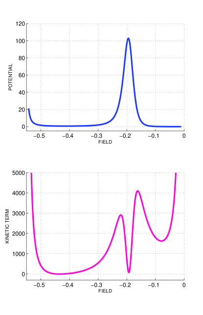
Figure 2: The potential and kinetic terms in the effective 4D theory for the initial theory (12) with the parameters $d=3,\ c=6.0,\ w_{1}=15,\ w_{2}=12,\ \Lambda=2.$

To illustrate the situation, consider a toy model of a scalar field $\phi$ with

$$V(\phi) \!= \!\frac{1}{2}m^{2}\phi^{2}$$

$${}K(\phi) \!= \!K_{1}\cdot(\phi-\phi_{\min})^{2}+K_{\min},\hskip 28.45274ptK_{1},\ K_{\min}>0.$$ (16)

Figure 3: Behaviour of the inflaton at the end of inflation for two models. 1. The standard kinetic term, $K=1/2$. 2. A kinetic term of the form (III.2). The parameters $K_{0}=0.1,\ \phi_{\min}=0.1,\ K_{\min}=0.005$ are given in Planck units, and time is measured in the units of inverse mass of the inflaton field. Both plots display the final stage of inflation lasting about 60 e-folds.

(The function $K(\phi)$ is positive and could be reduced to unity by the field redefinition $\phi\to\tilde{\phi}$, but this would be only another formulation of the same theory, less convenient for our purposes.)

Numerical solutions to the corresponding classical equations for spatially flat FRW cosmologies

$${}H^{2}=\frac{\varkappa^{2}}{3}\left[\frac{1}{2}K(\phi)\dot{\phi}^{2}+V(\phi)\right],$$

$${}K(\phi)\left(\ddot{\phi}+3H\dot{\phi}\right)+\frac{1}{2}K_{\phi}(\phi)\dot{\phi}^{2}+V_{\phi}(\phi)=0$$ (17)

(the index $\phi$ means $d/d\phi$, and $H$ is the Hubble parameter) are presented in Fig. 3 for quadratic potential (III.2) and two different kinetic terms: one with $K=1/2$ and the other given by (III.2), with parameter values given in the figure caption. Both plots display a few last e-folds of inflation and the consequent field oscillations. The nontrivial kinetic term $K(\phi)$ equals 1/2 at the end of inflation (the first point of line crossing in Fig. 3) for the chosen values of the parameters. Evidently, inflation in models with nontrivial kinetic terms starts at smaller energies as compared with the ordinary kinetic term, in agreement with the results obtained by Morris Morris in the framework of inflation at an intermediate scale.

An important observation is that in our case the frequency of inflaton oscillations is much larger than with the standard kinetic term, although inflation lasts for the same time. The resulting number of produced particles is proportional to this frequency, see the detailed review Dolgov and an additional discussion in Book1 . This conclusion could be qualitatively supported by the following argument.

When the inflation is over, the amplitude of inflaton oscillations is small on the Planck scale, and the effective kinetic term $K_{\rm eff}\sim K_{\min}$ is small due to the chosen values of the parameters. The effective Lagrangian, containing an interaction term of the inflaton and some other scalar field $\chi$

$$L_{\rm eff}\simeq\frac{1}{2}K_{\min}\dot{\phi}^{2}+g\phi\chi\chi,$$ (18)

can be transformed into the standard form by re-definition of the inflaton field:

$$L_{\rm eff}\simeq\frac{1}{2}\dot{\phi}^{2}+\frac{g}{\sqrt{K_{\min}}}\phi\chi\chi.$$ (19)

A small value of $K_{\min}$ increases the effective coupling constant (by an order of magnitude for the chosen values of the parameters) and surely leads to more intensive particle production. As a result, we overcome the difficulty discussed above: a slow motion during inflation may be reconciled with effective particle production right after inflation. Hence universes of this sort possess promising conditions for creation of complex structures.

IV A non-classical state near $K=0$

In this section we discuss the possible state of a universe near a node of the kinetic term. Ref. Kroger has indicated some consequences of singular points of kinetic terms in Einstein-scalar field theory. Recall that, in terms of Eq. (8), $K(\phi)=K_{\rm Ein}>0$ corresponds to a normal scalar field and $K(\phi)<0$ to a phantom field, with negative kinetic energy. Nodes and poles of $K(\phi)$ are of special interest. Let us show that such singular points of the kinetic term may take place in nonlinear gravity with extra dimensions.

To begin with, $F(R)$ theories considered in the previous sections produce only positive kinetic terms. Indeed, as is easily verified, the expression is square brackets in Eq. (9) is always positive, its minimum value being $d(d+3)/3$.

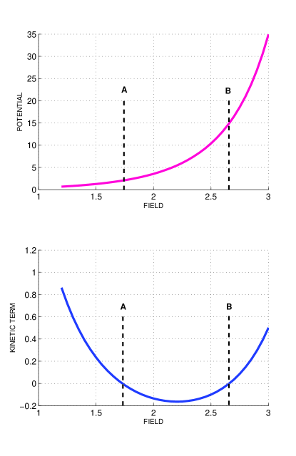
Figure 4: The potential (21) and the kinetic term (22) for the model (20) and $F(R)$ from (11). The parameters are $d=3,c=-0.12,\Lambda=2,c_{1}+c_{2}=-5.5$, $c^{\prime}=-0.626$.

However, if curvature-nonlinear terms in the Lagrangian exist due to quantum field effects, it seems reasonable to suppose that there can be contributions other than $F(R)$, and then the kinetic term of the effective theory is no more necessarily positive-definite. As an example, consider the simplest nonlinear theory (11) including additional nonlinear terms of quadratic order: the Ricci tensor squared $R_{AB}R^{AB}$ and the Kretschmann scalar ${\cal K}=R_{ABCD}R^{ABCD}$, so that

$$S=\int d^{D}x\sqrt{{}^{D}g}\left[F(R)+c_{1}R_{AB}R^{AB}+c_{2}{\cal K}\right].$$ (20)

Calculations for (20) with $F(R)$ given by (11) and the metric (2), similar to those made in Sec. 2, lead to an effective Einstein-scalar theory with

$$V_{\rm Ein}(\phi) \!= \!-\mathop{\rm sign}\nolimits(1+2c\phi)[d(d-1)]^{-d/2}\cdot|\phi|^{d/2}\frac{c^{\prime}\phi^{2}+\phi-2\Lambda}{(1+2c\phi)^{2}},$$ (21)

$${}\hskip 28.45274ptc^{\prime}=c+\frac{c_{1}}{d}+\frac{2c_{2}}{d(d-1)},$$

$${}K_{\rm Ein}(\phi) \!= \!\frac{1}{\phi^{2}(1+2c\phi)^{2}}\left[c^{2}\phi^{2}(d^{2}-2d+12)+d^{2}c\phi+\frac{1}{4}d(d+2)\right]+\frac{c_{1}+c_{2}}{2\phi(1+2c\phi)}.$$ (22)

In Fig. 4, the dashed lines A and B mark nodes of the kinetic term in the case of quadratic gravity (11). If a field fluctuation is produced to the left of line A, the field tends to the minimum of the potential located at $\phi=0$, corresponding to large extra dimensions. Some fluctuations are formed in the region between lines A and B, where the kinetic term is negative, the $\phi$ field is phantom and tends to climb the slope of the potential. If a fluctuation appears to the right of line B, it has a good opportunity to produce a universe with a nonzero cosmological constant. The ground state of such a universe is nontrivial and worth discussing in more detail.

To this end, consider a toy model with the action

$$S=\int d^{4}x\left[\frac{1}{2}K(\phi)(\partial\phi)^{2}-V(\phi)\right]$$ (23)

with $K(\phi_{\rm crit})=0$ by definition and, without loss of generality, suppose that $\phi_{\rm crit}=0$. Then the generic behaviour of $K(\phi)$ and $V(\phi)$ at small $\phi$ is $K(\phi)=k\phi+o(\phi)$ and $V(\phi)=V(0)+h\phi+o(\phi)$, where we put $k>0$, $h>0$ by analogy with point B in Fig. 4. Thus, near the critical point, the field tends upward if it is to the left of it and downward if it is to the right of it. In other words, the critical point looks like an attractor. Nevertheless, there is no classical motion near the point $\phi=0$. Indeed, the classical equation for $\phi$ in curved space-time has the general form

$$K(\phi)\mathop{\raisebox{-0.5pt}{$\Box$}}\nolimits\phi+\frac{1}{2}K_{\phi}(\partial\phi)^{2}=-V_{\phi},$$ (24)

or, according to the above expressions for $K$ and $V$ at small $\phi$,

$$k\phi\mathop{\raisebox{-0.5pt}{$\Box$}}\nolimits\phi=-\left(h+\frac{1}{2}k(\partial\phi)^{2}\right)+o(\phi).$$ (25)

Suppose that $(\partial\phi)^{2}>0$ (as is the case in cosmology when $\phi=\phi(t)$). Then the right-hand side of (25) is smaller than $-h<0$ and does not tend to zero as $\phi\to=0$. Hence the second derivatives involved in $\mathop{\raisebox{-0.5pt}{$\Box$}}\nolimits\phi$ tend to infinity as $\phi\to\phi_{\rm crit}=0$. One could improve the situation by invoking terms in the Lagrangian containing higher-order derivatives, making it possible to avoid infinite values of the derivatives, but it still remains unusual because a stationary state at the attractor is absent in any case. Indeed, if all derivatives are zero, the classical equation (25) with $h>0$ has no solution. It means that the kinetic energy of such a ground state cannot be zero. The problem obviously deserves a further study.

One can notice that a classical solution to Eq. (25) appears if $(\partial\phi)^{2}<0$, i.e., the field gradient is spacelike. It may thus happen that near the critical point there inevitably appear spatial inhomogeneities, which may lead to an instability.

V Alternative number and structure of extra dimensions

The previous section discussed effective low-energy theories corresponding to the metric (2) for different choices of the initial action. It is not surprising that some values of the parameters are suitable for the description of a universe like ours. Additional opportunities appear when varying the structure of extra dimensions, which includes the number of extra factor spaces, their dimensionality and curvature. Even if the initial Lagrangian is entirely specified, this additional freedom makes it possible to obtain low-energy effective Lagrangians drastically different from one another.

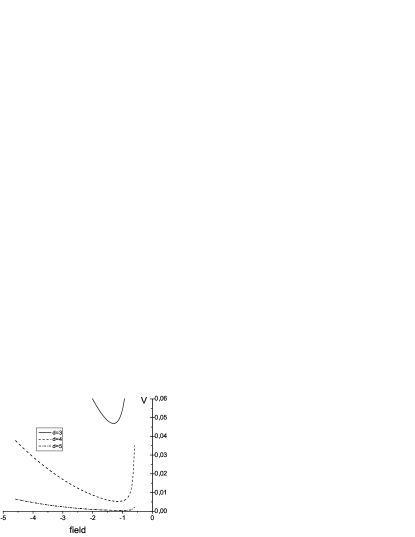
Figure 5: The effective potential $V(\phi)$ for different numbers of extra dimensions for the Lagrangian (8) with $F(R)$ of the from (11). Parameter values: $c=1,\ \Lambda=-0.4$.

V.1 Extra dimensions, inflaton mass and $\Lambda_{\rm eff}$

Let us start with discussing the well-known deficiency of chaotic inflation in its simplest, quadratic form. According to observations of the temperature fluctuations of the cosmic microwave background, the inflaton mass is about $10^{-6}\,m_{4}$. Its smallness needs an explanation. To this end, consider the effective potential (10) generated by the initial action (8), (11). Its shape is represented in Fig. 5 for some values of $d$, the number of extra dimensions. Evidently, one can fit the parameters in such a way that the potential does not contradict the observations. By increasing $d$, one could get an arbitrarily small values of the energy density at the minimum (at least in the Einstein frame). Its minimum can be made shallow to maintain small temperature fluctuation of the background radiation.

Simple numerical calculations give the following numbers: the second-order derivative at the bottom of the potential (in fact half mass of the inflaton) equals to $\sim 0.2m_{\scriptscriptstyle D}$ for $d=3$; $\sim 1.5\cdot 10^{-3}m_{\scriptscriptstyle D}$ for $d=5$ and $\sim 0.8\cdot 10^{-5}m_{\scriptscriptstyle D}$ for $d=7$. There are no small microscopic parameters in the Lagrangian. Nevertheless, a small inflaton mass arises at the classical level, and we can obtain appropriate conditions for the chaotic inflation in the early universe by choosing a sufficient number $d$ of extra dimensions. An estimate of this number depends on the uncertain ratio $m_{\scriptscriptstyle D}/m_{4}$; if $m_{\scriptscriptstyle D}\lesssim m_{4}$, the number $d=7$ suits.

A strong influence of the number $d$ on the effective Lagrangian parameters is not surprising since the potential (10) contains a quickly decreasing factor $\sim d^{-d}$. Thus, if in a stationary state $\phi=\phi_{0}$, the dimensionless initial parameters $|\phi_{0}|m_{\scriptscriptstyle D}^{-2}$ and $F^{\prime}(\phi_{0})$ are of order unity, the effective cosmological constant $\Lambda_{\rm eff}=V_{\rm Ein}(\phi_{0})$ is related to $F(\phi_{0})$ (which may be close to $m_{\scriptscriptstyle D}^{2}$) by

$$\Lambda_{\rm eff}/F(\phi_{0})\sim[d(d-1)]^{-d/2}.$$ (26)

It is of interest that $d^{-d}\approx 10^{-123}$ for $d=67$. Thus, at least in the Einstein picture, a fluctuation leading to a (67+4)-dimensional space, may evolve to a space with the vacuum energy density $10^{-123}\,m_{4}$. The extreme smallness of $\Lambda_{\rm eff}$ is related to the number of extra dimensions, and other physical ideas are not required. We have again taken for certainty $m_{\scriptscriptstyle D}=m_{4}$, otherwise the estimates will be slightly different.

Fig. 6 gives another example of $d$-dependence of the shape of the potential. Even its minimum does or does not exist depending on the value of $d$, see the curves at $\phi>0$. If a universe is nucleated with extra dimensions having negative curvature, we have $\phi<0$, see Fig. 6. Evidently the mean value of the potential $V(\phi)$ in such a universe tends to infinity for $d=2$, to a constant value for $d=4$ and to zero for $d=6$. All this takes place if the initial field value is less than $-1$. Otherwise, if a universe is born with $-1<\phi<0$, it is captured in a local minimum, and the size of extra dimensions remains small.

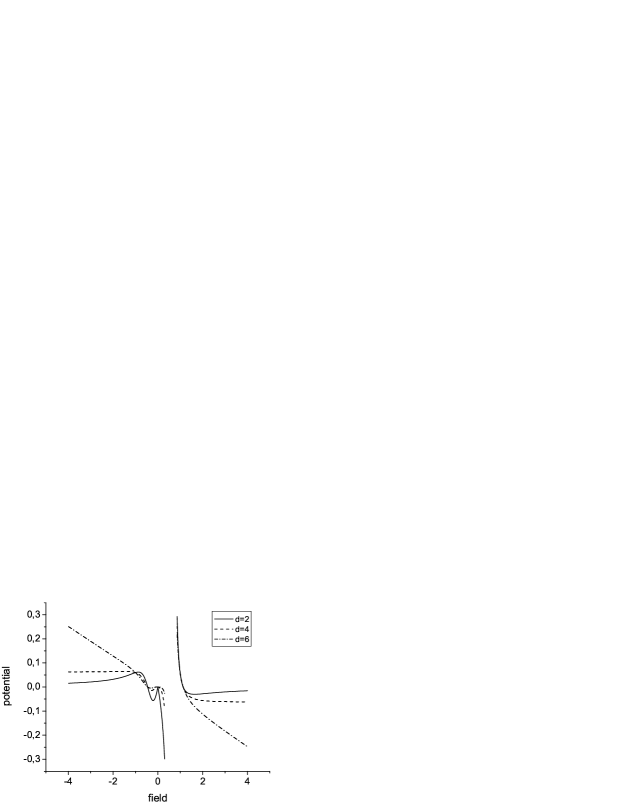
Figure 6: Different potentials for different $d$, obtained from the Lagrangian (8) with $F(R)$ in the form (12). Parameters: $c=0,\ w_{1}=0,\ w_{2}=-1,\ \Lambda=-0.25$. The curves are adapted to a unique scale.

One more example: extra dimensions with the topology of a 3-sphere. The effective potential (21) for this case is presented in Fig. 7 for positive field values. It has a metastable minimum, and a universe residing at this minimum as a ground state could live very long. As it was discussed in Section IIIA, such a universe could contain primordial massive black holes provided it was formed near the top of the potential.

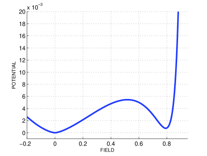
Figure 7: The effective potential (21). The parameters are: $c=-0.5,\ \Lambda=0.2,\ c^{\prime}=-0.626$, and $d=2$.

V.2 Multiple factor spaces and spatially dependent size of the extra dimensions.

As was mentioned in the Introduction, we do not assume a specific number of extra dimensions or their topology. Both are thought to arise due to quantum fluctuations close to the Planck scale. If quantum fluctuations lead to a more complex structure of the extra dimensions, the physics becomes much richer.

Consider an extra space with two factor spaces: ${\mathbb{M}}_{D}={\mathbb{M}}_{d_{1}}\times{\mathbb{M}}_{d_{2}}$. Treating the same action (20), we should introduce two scalar fields to describe the low-energy limit. The effective potential has the following form in the Einstein frame:

$${}V_{\rm Ein}(\phi_{1},\phi_{2})=-\frac{1}{2}\mathop{\rm sign}\nolimits\left(F^{\prime}(d_{1}\phi_{1}+d_{2}\phi_{2})\right)\frac{|\phi_{1}|^{d_{1}/2}}{[(d_{1}-1)]^{d_{1}/2}}\frac{|\phi_{2}|^{d_{2}/2}}{[(d_{2}-1)]^{d_{2}/2}}$$

$${}\hskip 72.26999pt\times\frac{F(d_{1}\phi_{1}+d_{2}\phi_{2})+d_{1}\phi_{1}^{2}[c_{1}+2c_{2}/(d_{1}-1)]+d_{2}\phi_{2}^{2}[c_{1}+2c_{2}/(d_{2}-1)]}{[F^{\prime}(d_{1}\phi_{1}+d_{2}\phi_{2})]^{2}},$$ (27)

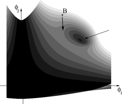
Figure 8: Effective potential for an extra space with the topology ${\mathbb{M}}_{D}={\mathbb{M}}_{d_{1}}\times{\mathbb{M}}_{d_{2}}$, $d_{1}=d_{2}=3$ and the parameters are $c=-0.5,\ \Lambda=0.2,\ c_{1}=c_{2}=-0.38$. The view is from above, lower levels are darker. The local minimum is marked by a long arrow.

It is represented in Fig. 8 where two valleys of the potential lie in perpendicular directions, $\phi_{1}=0$ and $\phi_{2}=0$, each of them corresponding to an infinite size of one of the extra factor spaces, ${\mathbb{M}}_{d_{1}}$ or ${\mathbb{M}}_{d_{2}}$. Of greater interest is the local minimum, marked by a long arrow, where both factor spaces are compact and have a finite size. A universe can live long enough in this metastable state, as in the case of a simpler topology of extra dimensions discussed above.

An interesting possibility arises if a universe is formed at point B in Fig. 8. There occurs inflation, and it ends as the fields move from point B along the arrow. The fate of different spatial domains depends on the field values in these domains. Even if most of them evolve to the metastable minimum, some part of the domains overcomes the saddle and tend to the first or second valley, with an infinite size of one of the factor spaces. In this case, our Universe should contain some domains of space with macroscopically large extra dimension. Their number and size crucially depend on the initial conditions.

The laws of physics in such a domain are quite different from ours. So, if, say, a star enters into such a domain, since the law of gravity is dimension-dependent, the balance of forces inside the star will be violated, and it will collapse or decay. More than that, there will be no usual balance between nuclear and electromagnetic forces in the stellar matter, so that even nuclei (except maybe protons) will decay as well. Even hadrons, being composite particles, are likely to lose their stability.

To conclude, we have seen that the same theory described by a specific Lagrangian leads to a diversity of low-energy situations, depending on the structure of extra dimensions and the initial conditions.

VI Conclusion

We have discussed the ability of nonlinear multidimensional gravity to produce various low-energy theories, some of which could describe our Universe. We only assume a certain form of the pure gravitational action and a sufficient number of extra dimensions in a Kaluza-Klein type framework, but do not fix the number, dimensions and curvature signs of extra factor spaces. Artificial inclusion of matter fields is not supposed, so that our conclusions are based on purely geometric grounds.

This problem setting creates a number of promising low-energy theories. We have discussed both some new effects and those already known, the latter being confirmed in the framework of multidimensional gravity.

First, we confirm the existence of de Sitter vacua studied in our paper BR06 in a wide range of parameters.

Second, nontrivial forms of the kinetic term of the inflaton field arise naturally in this approach. As a result, inflaton oscillations at the end of inflation could be very rapid with an appropriate form of the kinetic term. This increases the particle production rate after the end of inflation. At the same time, a slow motion of the inflaton at the beginning of inflation provides a sufficiently long inflationary stage.

Third, it has been shown that multiple production of closed walls and hence massive primordial black holes is a probable consequence of modern models of inflation. Their abundance strictly depends on the initial conditions and the input parameters of the model. This point must be taken into account in any model of inflation containing a potential with at least two minima.

Fourth, in the framework of multidimensional gravity, the effective kinetic term can change its sign, and its nodes are points of special interest. It has been shown that such a node can be considered as an attractor with a quantum/chaotic behaviour of the scalar field in its vicinity. The ground state energy of such a system turns out to be time-dependent, revealing a chaotic behaviour near the critical point.

Fifth, quite different effective low-energy models arise if one considers different numbers and/or topology of extra dimensions, even if all parameters of the initial Lagrangian are fixed. It means that the specific values of these parameters could be less important than it is usually supposed: even more important are the number, dimensions and curvatures of the extra factor spaces. In particular, varying the number $d$ of extra dimensions forming a single factor space, it is quite easy to obtain the proper value of the inflaton mass. Moreover, the problem of the tiny value of the observed cosmological constant may be explained (at least in the Einstein picture) by a moderate number of extra dimensions: by our estimate it suffices to have $d=67$, which, though also does not look attractive, can hardly be called an “astronomically large parameter”.

Sixth, if we take into account that the size of extra dimensions may depend on the spatial point in the observed space, our Universe may contain spatial domains with a macroscopic size of extra dimensions, where the whole physics should become effectively multidimensional. Matter (be it a spacecraft, a star or a galaxy) getting into such a domain would be unable to survive in its usual form.

Thus pure multidimensional gravity, even without any other ingredients, is quite a rich structure, and many problems of modern cosmology may be addressed in this framework. A task of interest is to try to construct a model able to solve a number of problems (if not all) simultaneously.

VII Acknowledgement

S.R. is grateful for the stimulating environment, hospitality and partial financial support provided by the Department of Physics of Manhattan College. K.B. acknowledges partial financial support from DFG Project No. 436RUS113/807/0-1(R) and Russian Basic Research Foundation Project No. 05-02-17478.

References

- (1) W. Lerche, D. Lust and A. N. Schellekens, Chiral four-dimensional heterotic strings from selfdual lattices, Nucl. Phys. B 287, 477 (1987).
- (2) S. Kachru, R. Kallosh, A. Linde and S. P. Trivedi, De Sitter vacua in string theory, Phys. Rev. D 68, 046005 (2003); hep-th/0301240.
- (3) S.G. Rubin, Fine tuning of parameters of the universe. Chaos Solitons Fractals 14, 891, 2002; astro-ph/0207013; S.G. Rubin, Origin of universes with different properties, Grav. & Cosmol. 9, 243-248, 2003; hep-ph/0309184].
- (4) A.A. Grib, S.G. Mamayev and V.M. Mostepanenko, “Vacuum Quantum Effects in Strong Fields”, Friedmann Laboratory Publ., St. Petersburg, 1994.
- (5) N.D. Birrell and P.C.W. Davies, Quantum Fields in Curved Space. Cambridge-London-New York-Sydney, Cambridge Univ. Press, 1982.
- (6) K.A. Bronnikov and S.G. Rubin, Self-stabilization of extra dimensions, Phys. Rev. D 73, 124019 (2006); gr-qc/0510107.
-
(7)
A. Starobinsky, Phys. Lett. B 91, 99–102, 1980;
A.H. Guth, Phys. Rev. D 23, 347–356, 1981;
A. Linde, Phys. Lett. B 108, 389–393, 1982; Phys. Lett. B 129, 177–181, 1983;
A. Albrecht and P. Steinhardt, Phys. Rev. Lett., 48, 1220–1223, 1982. - (8) L.F. Abbott and S-Y. Pi, Inflationary cosmology, World Scientific, 1986.
- (9) L. Alabidi and D.H. Lyth, Inflation models after WMAP year three, astro-ph/0603539.
- (10) A.D. Linde, Phys. Lett. B259, 38 (1991).
-
(11)
U. Günther, P. Moniz and A. Zhuk, “Multidimensional cosmology and
asymptotical ADS”, Astrophys. Space Sci. 283, 679-684
(2003); gr-qc/0209045;
U. Günther and A. Zhuk, “Remarks on dimensional reduction in multidimensional cosmological models”, gr-qc/0401003. - (12) R. Holman et.al, Phys. Rev. D 43,, 1991.
- (13) A.S. Majumdar and S.K. Sethi, Phys. Rev. D 46,, 5315, 1992.
- (14) A.S. Majumdar astro-ph/9905159.
- (15) H. Kroger, G. Melkonian, S.G. Rubin, Cosmological dynamics of scalar field with non-minimal kinetic term. Gen. Rel. Grav. 36, 1649-1659 (2004); astro-ph/0310182.
- (16) S.G. Rubin, Massive primordial black holes in hybrid inflation. In: *Moscow 2003, I. Ya. Pomeranchuk and physics at the turn of the century* 413-418; astro-ph/0511181.
- (17) A. Vilenkin, Phys. Rev. Lett. 74, 846 (1995).
- (18) M.Yu. Khlopov, S.G. Rubin, Cosmological Pattern of Microphysics in the Inflationary Universe. Dordrecht, Netherlands: Kluwer Academic (2004) 283 p. (Fundamental theories of physics. 144); S.G. Rubin, A.S. Sakharov and M.Yu. Khlopov, JETP 92, 921 (2001).
- (19) Lev Kofman, Andrei Linde and Alexei Starobinsky, Reheating after Inflation, Phys. Rev. Lett. 73, 3195-3198 (1994); hep-th/9405187.
- (20) G. Dvali and S. Kachru, astro-ph/0309095.
- (21) J.J. Blanco-Pillado et. al., JHEP 0411, 063 (2004); hep-th/0406230.
- (22) C.G. Callan and S.R. Coleman, Phys. Rev. D 16, 1762 (1977).
-
(23)
R.V. Konoplich and S.G. Rubin,
Sov. J. Nucl. Phys. 44, 359 (1986);
R.V. Konoplich, Theor. Mat. Fiz. 73, 1286 (1987). -
(24)
L. Amendola, E.W. Kolb, M. Litterio and F. Occhionero,
Phys. Rev. D 42, 1944, 1990;
L. Amendola, C.Baccigalupi, R.Konoplich, F.Occhionero, and S.Rubin, Phys. Rev. D 54, 7199 1996. - (25) J. Baacke and G. Lavrelashvili, Phys. Rev. D 69, 125009 (2004).
- (26) G.V. Dunne and H. Min, Phys. Rev. D 72, 125004 (2005).
- (27) Ya.B. Zeldovich, I.Y. Kobzarev and L.B. Okun, Sov. Phys. JETP 40, 1 (1975).
- (28) A. Starobinsky, in Field Theory, Quantum Gravity and Strings, ed. H.J. de Vega and N. Sanchez, 107-126, 1986.
- (29) V. Dokuchaev, Y. Eroshenko and S. Rubin, Grav. & Cosmol. 11, 99-104 (2005); astro-ph/0412418.
- (30) J. Morris, “Generalized slow roll conditions and the possibility of intermediate scale inflation in scalar-tensor theory”, Class. Quantum Grav. 18, 2977–2988, 2001; gr-qc/0106022
-
(31)
P.J. Steinhardt, UPR-0198T, Invited talk given at Nuffield
Workshop on the Very Early Universe, Cambridge, England, Jun 21 -
Jul 9, 1982;
A.D. Linde, Print-82-0554 (Cambridge);
A. Vilenkin, Phys. Rev. D 27, 2848 (1983). -
(32)
A.D. Dolgov and A.D. Linde, Phys. Lett. 116B, 329 (1982);
L.F. Abbott, E. Fahri and M. Wise, Phys. Lett. 117B, 29 (1982). - (33) Y. Shtanov, J. Traschen and R. Brandenberger, Universe reheating after inflation, hep-ph/9407247.
- (34) A. Dolgov, F. Freese, R. Rangarajan, and M. Srednicki, hep-ph/9610405.