Two-dimensional gravity with a dynamical aether

Abstract

We investigate the two-dimensional behavior of gravity coupled to a dynamical unit timelike vector field, i.e. “Einstein-aether theory”. The classical solutions of this theory in two dimensions depend on one coupling constant. When this coupling is positive the only solutions are (i) flat spacetime with constant aether, (ii) de Sitter or anti-de Sitter spacetimes with a uniformly accelerated unit vector invariant under a two-dimensional subgroup of $SO(2,1)$ generated by a boost and a null rotation, and (iii) a non-constant curvature spacetime that has no Killing symmetries and contains singularities. In this case the sign of the curvature is determined by whether the coupling is less or greater than one. When instead the coupling is negative only solutions (i) and (iii) are present. This classical study of the behavior of Einstein-aether theory in 1+1 dimensions may provide a starting point for further investigations into semiclassical and fully quantum toy models of quantum gravity with a dynamical preferred frame.

Theories of gravity in two spacetime dimensions have provided useful toy models for the investigation of issues such as black hole evaporation and information loss, singularities, and quantization of gravity, in a setting where some of the technical problems that arise in four dimensions are absent. In two dimensions the Einstein-Hilbert action is topological, so something else must be used. An early proposal was the Jackiw-Teitelboim model JT , for which the equations of motion imply the metric has a fixed constant curvature specified by a parameter in the Lagrangian. A generalization of this idea is dilaton gravity Grumiller:2002nm , which is a class of models that incorporates a scalar field in addition to the metric. These theories possess no local degrees of freedom, but there exist for example black hole solutions Grumiller:2002nm ; Brown:1986nm ; Frolov:1992xx ; Callan:1992rs ; Achucarro:1993fd , and when coupled to matter fields the theories acquire local dynamics.

In this paper we examine the two dimensional version of “Einstein-aether” theory, which is a generally covariant theory consisting of general relativity coupled to a dynamical unit timelike vector field $u^{a}$. Our motivation is that, like other two dimensional models, this might provide a useful setting in which to study aspects of quantum gravity. A special feature of this theory is the presence of the unit timelike vector field, which might ameliorate or modify the problem of time in the canonically quantized setting. The vector also defines an intrinsic preferred frame with which for example the impact of Lorentz violation on black hole evaporation could be studied. The two dimensional case provides the simplest context in which to begin examining this idea. It may also be relevant to the spherical reduction of the higher dimensional theory. For a review of motivations, history and status of the 3+1 dimensional Einstein-aether theory as of 2004 see Eling:2004dk and the references therein. A more recent brief review with further references is given in the introduction of Eling:2006df .

A unit vector field in two dimensions has only one degree of freedom, so in this respect is similar to a dilaton field. Like the dilaton, the presence of the vector field renders the theory nontrivial, but still with no local degrees of freedom. However, Einstein-aether theory seems to provide a different two dimensional gravity model than any previously considered. It possesses both constant and non-constant curvature solutions. Unlike the Jackiw-Teitelboim model the constant curvature is not specified a priori by the action. In this regard it is similar to two-dimensional unimodular gravity unimod , but unlike in unimodular gravity the sign of the curvature scalar is determined by the action. Also it has the unit vector field, which defines in each solution a locally preferred frame. The gradient of a dilaton field also defines a vector, and so we looked for a correspondence between unimodular dilaton gravity and ae-theory in two dimensions, but so far have not identified any precise mapping between the theories.

I 1+1 dimensional action

The action for Einstein-aether theory in $n$ dimensions is

$$S[g_{ab},u^{a},\lambda]=\frac{-1}{16\pi G}\int d^{n}x\,\sqrt{-g}\Bigl{(}R+L_{u}+\lambda(g_{ab}u^{a}u^{b}-1)\Bigr{)},$$ (1)

where $R$ is the Ricci scalar, $\lambda$ is a Lagrange multiplier enforcing the unit timelike constraint on $u^{a}$, and the aether Lagrangian is defined by

$$L_{u}=c_{1}(\nabla_{a}u_{b})(\nabla^{a}u^{b})+c_{2}(\nabla_{a}u^{a})^{2}+c_{3}(\nabla_{a}u_{b})(\nabla^{b}u^{a})+c_{4}(u^{a}\nabla_{a}u^{b})(u^{c}\nabla_{c}u_{b})$$ (2)

where the $c_{i}$ are dimensionless coupling constants, and $\lambda$ is a Lagrange multiplier. Here we use the signature $({+}{-}\cdots{-})$. This action includes all generally covariant terms with up two two derivatives (not including total divergences) that can be constructed from a metric and a unit vector field.

In two-dimensional spacetime the variation of the Einstein-Hilbert term $\sqrt{-g}R$ is a total divergence. The aether part of the action is non-trivial, but only two of the terms are independent. To see this we express the covariant derivative $\nabla_{a}u_{b}$ in the orthonormal basis $\{u^{a},s^{a}\}$, where $s^{a}$ is a unit spacelike vector orthogonal to $u^{a}$. It follows from $u^{a}u_{a}=-s^{a}s_{a}=1$ and $u^{a}s_{a}=0$ that $0=u^{b}\nabla_{a}u_{b}=s^{b}\nabla_{a}s_{b}=u^{b}\nabla_{a}s_{b}+s^{b}\nabla_{a}u_{b}$ everywhere. Using these relations, we find that when the unit constraint is satisfied the covariant derivatives take the form

$$\nabla_{a}u_{b} = As_{a}s_{b}+Bu_{a}s_{b},$$ (3)

$$\nabla_{a}s_{b} = As_{a}u_{b}+Bu_{a}u_{b}.$$ (4)

where $A$ and $B$ are generically spacetime functions. Using (3) we obtain

$$(\nabla_{a}u_{b})(\nabla^{a}u^{b}) = A^{2}-B^{2}$$ (5)

$$(\nabla_{a}u_{b})(\nabla^{b}u^{a}) = A^{2}$$ (6)

$$(\nabla_{a}u^{a})^{2} = A^{2}$$ (7)

$$(u^{a}\nabla_{a}u^{b})(u^{c}\nabla_{c}u_{b}) = -B^{2}$$ (8)

$$F_{ab}F^{ab} = -2B^{2},$$ (9)

where $F_{ab}=\nabla_{a}u_{b}-\nabla_{b}u_{a}$. These expressions may be substituted into the Lagrangian (2) without changing the equations of motion, since the Lagrange multiplier term in the action (1) implies that the equations of motion are equivalent to the condition that the action be stationary only with respect to variations of $u^{a}$ that preserve the constraint $u^{a}u_{a}=1$. On the constraint surface the Lagrangian is thus given by

$$L_{u}=c_{123}A^{2}-c_{14}B^{2},$$ (10)

where $c_{123}\equiv c_{1}+c_{2}+c_{3}$ and $c_{14}\equiv c_{1}+c_{4}$. Using (7) and (9) the Lagrangian can therefore be written for example as

$$L_{u}={\textstyle{\frac{1}{2}}}c_{14}F^{ab}F_{ab}+c_{123}(\nabla_{a}u^{a})^{2},$$ (11)

without any loss of generality in the theory.

If either $c_{14}$ or $c_{123}$ vanishes the theory is under-deterministic. In particular, if $c_{123}=0$ then obviously any metric and unit vector satisfying $F_{ab}=0$ obey all the field equations with $\lambda=0$. If instead $c_{14}=0$ then then any metric and unit vector satisfying $\nabla_{a}u^{a}=0$ obey all the field equations with $\lambda=0$. (In fact, these include all solutions.) We thus assume in the remainder of this paper that neither $c_{14}$ nor $c_{123}$ is zero. The classical equations of motion then depend only on the one combination $c_{123}/c_{14}$ of the coupling coefficients.

The action can be further simplified by a field redefinition of the form

$$g_{ab} = g^{\prime}_{ab}+(\sigma-1)u^{\prime}_{a}u^{\prime}_{b}$$

$$u^{a} = \sigma^{-1/2}u^{\prime a}.$$ (12)

Here the coefficient $\sigma$ must be positive in order to preserve Lorentzian signature. This redefinition preserves the general form of the action given in (1), the overall effect being only a change of the coupling constants,

$$S[g_{ab},u^{a},c_{i}]=S[g^{\prime}_{ab},u^{\prime a},c^{\prime}_{i}(c_{i},\sigma)].$$ (13)

The relation between $c^{\prime}_{i}$ and $c_{i}$ was found by FosterFoster:2005ec , and is most usefully specified by certain linear combinations that have simple transformation behavior,

$$c^{\prime}_{14} = c_{14}$$ (14)

$$c^{\prime}_{123} = \sigma^{-1}c_{123}$$ (15)

$$c^{\prime}_{13}-1 = \sigma^{-1}(c_{13}-1)$$ (16)

$$c^{\prime}_{1}-c^{\prime}_{3}-1 = \sigma(c_{1}-c_{3}-1).$$ (17)

This result applies in any spacetime dimension. The $c^{\prime}_{i}$ receive contributions from the $R$ term in the action which appear in (16) and (17) via the $c_{i}$–independent terms. However in 1+1 dimensions these contributions cannot affect the equations of motion since as noted above the variation of the $R$ term is a total divergence. Indeed, the Lagrangian (11) depends only on the two combinations $c_{14}$ and $c_{123}$ whose transformation has no $c_{i}$–independent terms.

Since $c_{14}$ is invariant and $c_{123}$ simply scales by the nonzero factor $\sigma^{-1}$, no field redefinition will make one of the terms in (10) or (11) vanish. On the other hand, the choice $\sigma=c_{123}/c_{14}$ (which is allowed as long as it is positive) will produce $c^{\prime}_{14}=c^{\prime}_{123}$, in which case using (5) the Lagrangian may be reduced to just one term of the original four-term Lagrangian (2),

$$L_{u,{\rm reduced}}=c^{\prime}_{14}(\nabla_{a}u_{b})(\nabla^{a}u^{b})=c^{\prime}_{14}\bigl{(}F^{ab}F_{ab}+(\nabla_{a}u^{a})^{2}).$$ (18)

In terms of the new fields the classical equations of motion are thus totally independent of the coupling parameters. We shall obtain the solutions for the general case when $c_{123}/c_{14}$ is positive by applying the field redefinition to solutions of this reduced theory.

II Field equations and solutions

In this section we will study the general two-dimensional theory described by the action with Lagrangian (11), to obtain the field equations and the curvature of their solutions. The Lagrangian takes the form

$$L_{u}=c_{14}\left({\textstyle{\frac{1}{2}}}F^{ab}F_{ab}+\beta(\nabla_{a}u^{a})^{2}\right),$$ (19)

where

$$\beta=c_{123}/c_{14}.$$ (20)

The equations of motion depend on the couplings only through the combination $\beta$ defined in (20). Varying with respect to the inverse metric $g^{ab}$ and the covariant aether vector $u_{a}$ as independent field variables, we find the metric field equation

$$F_{am}F_{b}{}^{m} - {\textstyle{\frac{1}{2}}}g_{ab}({\textstyle{\frac{1}{2}}}F^{ab}F_{ab}-\beta(\nabla_{c}u^{c})^{2}-2\beta u^{m}\nabla_{m}(\nabla_{c}u^{c}))$$ (21)

$$- 2\beta u_{(a}\nabla_{b)}\nabla_{c}u^{c}+\lambda u_{a}u_{b}=0$$

and the aether field equation

$$\nabla_{b}F^{ba}+\beta\nabla^{a}(\nabla_{c}u^{c})-\lambda u^{a}=0,$$ (22)

where $\lambda$ is a re-scaled Lagrange multiplier (cf. eqn. (1)). These amount to three equations from (21) and two from (22). The $u^{a}$ component of the latter determines $\lambda$. Using the expansion of the covariant derivatives (3,4) to project out the various components of the field equations we find that the remaining four equations are equivalent to

$$uA=f\qquad sA=0,$$ (23)

$$uB=0\qquad sB=\beta f$$

where (for example) $uA\equiv u^{m}\nabla_{m}A$, and

$$f\equiv{\textstyle{\frac{1}{2}}}(A^{2}-\beta^{-1}B^{2}).$$ (24)

The equations (23) are extremely restrictive, and there are just two types of solutions. In the first type both $A$ and $B$ are constant and related by $B^{2}=\beta A^{2}$ so that $f=0$. In the second type of solution the gradients $\nabla_{a}A$ and $\nabla_{b}B$ are both non-zero and independent. In this case $A$ and $B$ may be used as coordinates, so one can immediately write the unique solution,

$$u=f\partial_{A}\qquad\mbox{and}\qquad s=\beta f\partial_{B}.$$ (25)

The inverse metric is given by $g^{ab}=u^{a}u^{b}-s^{a}s^{b}$, hence for this solution the line element is

$$ds^{2}=\frac{4}{(\beta A^{2}-B^{2})^{2}}(\beta^{2}dA^{2}-dB^{2}).$$ (26)

The scalar curvature $R$ completely characterizes the curvature in two-dimensions. Using the relation

$$R=2u^{a}(\nabla_{b}\nabla_{a}-\nabla_{a}\nabla_{b})u^{b}$$ (27)

which is valid in two-dimensions, and making use of (3) and (4), we find

$$R=2(B^{2}-A^{2}+uA+sB).$$ (28)

When the field equations (23) are satisfied the scalar curvature is thus given by

$$R=(\beta-1)A^{2}+(1-\beta^{-1})B^{2}.$$ (29)

The solutions with constant $A$ and $B$ thus have constant curvature. Being two dimensional, they are therefore either Minkowski, de Sitter, or anti-de Sitter space, and have three independent Killing vectors. The solution (26) has non-constant curvature unless $\beta=1$, in which case it is flat. For $\beta\neq 1$ it can be shown that (26) has no Killing vectors. For $\beta>1$ the curvature scalar is positive, for $0<\beta<1$ it is negative, and for $\beta<0$ it is indefinite.

In the case $\beta<0$ the function $f$ defined in (24) can only vanish when both $A$ and $B$ vanish, hence the only solution with constant $A$ and $B$ is the one with $A=B=0$. In this solution the metric is flat, and according to (3) the vector field $u^{a}$ is then constant. The only other solution in this case is (25,26). The curvature scalar for this metric with $\beta<0$ is zero on the lines $|B|=|A|(1-\beta)/(1-\beta^{-1})$, negative for smaller $|B|/|A|$ and positive for larger $|B|/|A|$. It vanishes at $A=B=0$, which lies at infinite distance diverging as $1/A$ on any non-null line $A/B={\rm const}$. There is a curvature singularity as either $A$ or $B$ goes to infinity, except on the lines where the curvature vanishes, and the geodesic distance to this singularity is finite.

In the next section we determine the nature of the solutions for the special case $\beta=1$, and the following section addresses the case $0<\beta\neq 1$. Since the Lagrangian with $\beta>0$ can be reached by a field redefinition from the $\beta=1$ case, the solutions for general positive $\beta$ can be obtained by field redefinition from the $\beta=1$ solutions.

III $\beta=1$: Flat spacetime solutions

To find the solutions in the case $\beta=1$, for which the curvature vanishes, we adopt null coordinates $(w,v)$, so

$$ds^{2} = dw\,dv$$ (30)

$$u = F\partial_{w}+F^{-1}\partial_{v}$$ (31)

where $F(w,v)$ is to begin with an arbitrary function. The functions $A$ and $B$ defined in (3) and (4) are then given by

$$A = -F_{,w}+F^{-2}F_{,v}$$

$$B = F_{,w}+F^{-2}F_{,v}.$$ (32)

Using the field equations in the form (23) with $\beta=1$, we find that $uB+sA=0$ implies $(\log F)_{,wv}=0$, $(u+s)(A-B)=0$ implies $F_{,ww}=0$, and $(u-s)(A+B)=0$ implies $(1/F)_{,vv}=0$. It follows that the general solution is

$$F=(a+bw)/(c+dv),$$ (33)

where $a,b,c,d$ are constants. Thus there are four classes of solutions for $u^{a}$, corresponding to whether or not the constants $b$ and $d$ vanish. Up to constant coordinate shifts and opposite scalings of $w$ and $v$ (which preserve the Minkowski metric (30)) these four solutions have $(w,v)$ components

$$(1,1)$$ (34)

$$(kw,(kw)^{-1})$$ (35)

$$((kv)^{-1},kv)$$ (36)

$$(w/v,(w/v)^{-1})$$ (37)

where $k$ is a constant with dimensions of inverse length that sets a physical scale for the solution.

The first solution (34) is simply a constant vector field covering the entire Minkowski spacetime. In this solution $A$ and $B$ both vanish. The second and third solutions (35) and (36) are equivalent to each other with the roles of $w$ and $v$ reversed. For the solution (35) we use (32) to find that $A=-B=-k$, so these are solutions of the type with $A$ and $B$ constant. In the solution (35) the vector field $u^{a}$ is non-singular in regions covering one-half of the flat Minkowski manifold, either $w>0$ or $w<0$. Along the line $w=0$ the vector $u^{a}$ becomes infinitely stretched in order to maintain unit norm as it aligns with the null vector $\partial_{v}$. There is a similar divergence as $w\rightarrow\pm\infty$ where $u^{a}$ aligns with $\partial_{w}$. The flow lines of $u^{a}$ are the level curves of a function $\Phi$ with $u\Phi=kw\Phi_{,w}+(kw)^{-1}\Phi_{,v}=0$, which is satisfied by $\Phi=v+(k^{2}w)^{-1}$. Thus the flow lines are given by

$$v+(k^{2}w)^{-1}={\rm const.}$$ (38)

These curves are hyperbolae, as can also be seen from the fact that the acceleration vector $u^{a}\partial_{a}u^{b}$ is given in $(w,v)$ components by $kw\partial_{w}(kw,(kw)^{-1})=(k^{2}w,-w^{-1})$, which has the constant squared norm $-k^{2}$. A plot showing these flow lines in a part of the Minkowski space is shown in Fig. 1.

Figure 1: Plot of the flow lines of (35) in Minkowksi space with Cartesian coordinates $t$ (increasing vertically) and $x$ (increasing toward the right). The $u^{a}$ field approaches the null vector $\partial_{v}$ along the line $w=t-x=0$, hence must be infinitely stretched there in order to maintain the unit constraint.

The solution (35) is further characterized by its symmetries. Being flat, the metric has two translational symmetries generated by the Killing vectors $\partial_{w}$ and $\partial_{v}$, and one boost symmetry generated by $w\partial_{w}-v\partial_{v}$. The vector field $u^{a}$ is clearly invariant under $\partial_{v}$, since its components depend only upon $w$. It is also invariant under the boost Killing vector: $[w\partial_{w}-v\partial_{v},kw\partial_{w}+(kw)^{-1}\partial_{v}]=0$. The commutator of these two Killing vectors that commute with $u^{a}$ is

$$[w\partial_{w}-v\partial_{v},\partial_{v}]=\partial_{v}.$$ (39)

They generate a non-abelian sub-algebra of the Poincare algebra in 1+1 dimensions. This sub-algebra is isomorphic to the algebra of the affine group $A(1)$ of translations and scalings in one dimension. It will re-appear in the next section as a sub-algebra of the 2+1 dimensional Lorentz group when we relate this solution to a constant curvature one via a field redefinition.

For the fourth solution (37) we again use (32) to find that now

$$A = -w^{-1}-v^{-1}$$

$$B = -w^{-1}+v^{-1}.$$ (40)

These are not constant, so this solution corresponds to the solution (25,26) with $\beta=1$. Though not obviously flat, this line element is evidently related to the Minowski metric by the coordinate transformation (40). The vector field $u^{a}$ in this solution is singular on both lines $w=0$ and $v=0$, and stretches infinitely as either $v$ or $w$ goes to infinity. The solution is thus regular in any of the four wedges $(w>0,v>0)$, $(w<0,v<0)$, $(w>0,v<0)$, and $(w<0,v>0)$. The first two are related by time reflection and the last two by space reflection, but the first pair is physically distinct from the second pair. The flow lines in this case are the level curves of a function $\Phi$ with $u\Phi=(w/v)\Phi_{,w}+(v/w)\Phi_{,v}=0$, which is satisfied by $\Phi=w^{-1}-v^{-1}$. The flow lines are therefore given by

$$w^{-1}-v^{-1}={\rm const.}$$ (41)

These curves do not have constant acceleration. A plot showing them in a part of the Minkowski space is shown in Fig. 2. Unlike the previous case, this $u^{a}$ field commutes with none of the Killing vectors of the flat metric.

Figure 2: Plot of the flow lines of (37) in Minkowksi space with Cartesian coordinates $t$ and $x$. Here the aether is singular along the lines $w=t-x=0$ and $v=t+x=0$.

This completes our analysis of the solutions in the special case when the coupling constants satisfy $\beta=1$, for which the metric is flat. Next we turn to determining the solutions for general $\beta>0$.

IV $0<\beta\neq 1$ solutions

To obtain the general solutions for the theory when $0<\beta\neq 1$ we use the field redefinition (12) with $\sigma=\beta$,

$$g_{ab} = \eta_{ab}+(\beta-1)u^{\prime}_{a}u^{\prime}_{b}$$

$$u^{a} = \beta^{-1/2}~{}u^{\prime a}.$$ (42)

If $(\eta_{ab},u^{\prime a})$ is a solution to the theory with $\beta=1$ then $(g_{ab},u^{a})$ is a solution with arbitrary positive $\beta=c_{123}/c_{14}$. Conversely, every solution of the $\beta\neq 1$ theory can be obtained in this way. We apply this method to the three different types of solutions found in the previous section.

Under the field redefinition (42) the new line element is

$$ds^{2}={\textstyle{\frac{1}{4}}}(\beta-1)(u^{\prime w})^{-2}dw^{2}+{\textstyle{\frac{1}{2}}}(\beta+1)dwdv+{\textstyle{\frac{1}{4}}}(\beta-1)(u^{\prime w})^{2}dv^{2}$$ (43)

and the new aether is

$$u=\beta^{-1/2}(u^{\prime w}\partial_{w}+u^{\prime v}\partial_{v}),$$ (44)

where we use the same coordinates $(w,v)$ to describe the new solution as we used for the flat one. The determinants of both the primed (flat) and unprimed metrics are constant in these coordinates, hence we have $\nabla_{a}u^{a}=\nabla^{\prime}_{a}u^{a}$ and similarly for $s^{a}$, so using (3), (4) and (42) we find

$$A=\beta^{-1/2}A^{\prime}\qquad\mbox{and}\qquad B=B^{\prime}.$$ (45)

The curvature (29) of the new metric is therefore given by

$$R=(1-\beta^{-1})(A^{\prime 2}+B^{\prime 2}),$$ (46)

where $A^{\prime}$ and $B^{\prime}$ are those of the primed, flat solution (which had $\beta=1$).

For the constant vector field solution (34) the primed metric components remain constant, as do those of the aether, so after the field redefinition we still have the trivial solution of a constant aether in a flat spacetime after the field redefinition.

In the next two subsections we consider the solutions obtained by field redefinition from the other two types of solutions, first (37) and next (35) and (36).

IV.1 Non-constant curvature solution

Using (43) with the primed solution (37) we find

$$ds^{2}={\textstyle{\frac{1}{4}}}(\beta-1)(w/v)^{2}dw^{2}+{\textstyle{\frac{1}{2}}}(\beta+1)dwdv+{\textstyle{\frac{1}{4}}}(\beta-1)(v/w)^{2}dv^{2}$$ (47)

As we saw in (40) $A^{\prime}$ and $B^{\prime}$ are not constant for this $u^{\prime}$, hence according to (45) neither are $A$ and $B$, so this solution corresponds again to the non-constant curvature solution (26). The scalar curvature (46) of the new metric (47) is given, according to (46) and (40), by

$$R=2(1-\beta^{-1})(w^{-2}+v^{-2}).$$ (48)

As discussed in Section III, none of the flat-spacetime Killing vectors commute with this $u^{\prime a}$, from which it follows that no Killing vector of $g_{ab}$ could commute with $u^{a}$. Moreover, in fact $g_{ab}$ has no Killing vectors at all, as mentioned previously.

When $w$ or $v$ vanishes the metric (47) has a curvature singularity. In the same limits $u^{a}$ aligns with either $\partial_{w}$ or $\partial_{v}$, which are null vectors when respectively $w$ or $v$ equals zero. Thus, for this solution, the scalar curvature becomes singular exactly on the horizons where $u^{a}$ must be infinitely stretched. As in the flat case discussed above there are two distinct regular solutions (up to time or space reflection), corresponding to the coordinate ranges $w,v>0$ or $w<0,v>0$. Approaching the singularity at $w=0$ along a line of constant $w+v>0$, the distance diverges logarithmically as $\log w$. If instead we fix $w/v$ and go out to infinite values of $w$ and $v$ the curvature approaches zero, and the distance diverges linearly in $w$. On the other hand if we fix $w$ and go out to infinite $v$ the curvature approaches a constant proportional to $w^{-1}$ and the distance diverges as $\log v$.

IV.2 Constant curvature solutions

Under the field redefinition (42) the second type of solution (35) produces the metric

$$ds^{2}={\textstyle{\frac{1}{4}}}(\beta-1)(kw)^{-2}dw^{2}+{\textstyle{\frac{1}{2}}}(\beta+1)dwdv+{\textstyle{\frac{1}{4}}}(\beta-1)(kw)^{2}dv^{2}$$ (49)

and re-scaled $u^{a}$

$$u=\beta^{-1/2}(kw\partial_{w}+(kw)^{-1}\partial_{v}).$$ (50)

As mentioned in the previous section, (32) implies for the primed solution $A^{\prime}=-B^{\prime}=-k$, so according to (45) this solution corresponds to the general type with constants $A=-\beta^{-1/2}k$ and $B=k$, and the scalar curvature (46) of the primed metric (49) is

$$R^{\prime}=2(1-\beta^{-1})k^{2},$$ (51)

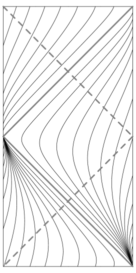
Figure 4: Conformal diagram of 1+1 AdS spacetime with the flow lines of the aether field. The two vertical lines at left and right are at null infinity, and the diagram should be continued infinitely in the vertical direction. The aether is regular in the Poincaré patch bounded by the solid grey lines and null infinity. The dashed grey lines are the rest of the boost Killing horizon. The diagram is drawn for the case $\beta=10$.

The curvature is constant, so the geometry is locally that of de-Sitter (dS) for $0<\beta<1$ and anti-de-Sitter (AdS) space for $\beta>1$ (Recall that we use the metric signature $(+{-})$, so the scalar curvature for dS is negative while for AdS it is positive.) The nature of these maximally symmetric spaces is well-known, so to fully describe these solutions we need only specify the behavior of the $u^{a}$ vector field on the dS/AdS background. This behavior is illustrated for the case of de Sitter and anti-de Sitter spaces in Fig. 3 and Fig. 4. In the remainder of this paper we explore the properties of this solution.

First note that since

$$u^{a}\nabla_{a}u_{b}=u^{a}(As_{a}s_{b}+Bu_{a}s_{b})=ks_{b}$$ (52)

the magnitude of the acceleration of the flow of $u^{a}$ with respect to $g_{ab}$ is constant and equal to $k$, as is that of $u^{\prime a}$ with respect to $\eta_{ab}$. The coordinates $w$ and $v$ in (49) are not null with respect to $g_{ab}$ since the effect of the $u^{\prime}_{a}u^{\prime}_{b}$ contribution to (42) is to narrow the light cones of the flat metric when $0<\beta<1$ and widen them when $\beta>1$. However, $\partial_{v}$ is a null vector when $w=0$ and similarly $\partial_{w}$ is null when $w\rightarrow\pm\infty$. From (50), it is clear that $u^{a}$ is singular on one of the dS/AdS horizons labelled by $w=0$, where it is infinitely stretched in order to remain unit timelike as it approaches a null vector. It is also infinitely stretched as $w$ approaches $\pm\infty$. The aether is thus regular in either of the two coordinate patches $w>0$ or $w<0$. It is not immediately clear to which regions of dS/AdS these patches correspond. We shall address this shortly with the help of new coordinates better adapted to the dS/AdS metric, but first let us examine the symmetries of the solutions.

IV.2.1 Symmetries of constant curvature solutions

Constant curvature dS/AdS manifolds are maximally symmetric and have three independent Killing vectors in 1+1 dimensions. In a flat 2+1 dimensional embedding space these generate the boosts and rotation in the $SO(2,1)$ or $SO(1,2)$ symmetry group that preserves the dS or AdS hyperboloid respectively. Two-dimensional dS and AdS are related by interchange of the spacelike and timelike dimensions so the corresponding solutions are closely related. We shall focus on the dS case here, and indicate the corresponding results for AdS at the end.

In terms of the Minkowski coordinates $X^{0}$, $X^{1}$, $X^{2}$ of the flat 2+1 dimensional spacetime the generators of $SO(2,1)$ are the two boosts $\textbf{K}_{1}=X^{0}\partial_{1}+X^{1}\partial_{0}$ and $\textbf{K}_{2}=X^{0}\partial_{2}+X^{2}\partial_{0}$, and one rotation $\textbf{J}=X^{1}\partial_{2}-X^{2}\partial_{1}$. These form the Lie algebra with commutators

$$[\textbf{K}_{1},\textbf{K}_{2}] =$$ J

$$\left[\textbf{J},\textbf{K}_{1}\right] = -\textbf{K}_{2}$$

$$\left[\textbf{J},\textbf{K}_{2}\right] = \textbf{K}_{1}.$$ (53)

We are interested in the subgroup under which also the aether is invariant. The corresponding Killing vectors are identical to the Killing vectors of $\eta_{ab}$ that commute with $u^{\prime a}$, since ${\cal L}_{\xi}\eta_{ab}={\cal L}_{\xi}u^{\prime}_{a}=0$ implies ${\cal L}_{\xi}g_{ab}={\cal L}_{\xi}u_{a}=0$. Their algebra is given by (39). These Killing vectors must generate a two dimensional non-Abelian subgroup of $SO(2,1)$. The only two-dimensional non-Abelian subalgebras of (53) are generated by a boost and a null rotation, for example

$$\left[\textbf{K}_{1},\textbf{J}+\textbf{K}_{2}\right]=\textbf{J}+\textbf{K}_{2}.$$ (54)

This coincides with the flat spacetime algebra (39) discussed in Section III, and so reveals the geometrical nature of the symmetry group of our solutions.

Acting with the null rotation $\textbf{J}+\textbf{K}_{2}$ as a differential operator one sees that the combination $X^{0}+X^{1}$ is invariant. Thus, the flow lines of this null rotation on the hyperboloid are the intersections of null planes $X^{0}+X^{1}=\rm{const.}$ with the embedded hyperboloid. We shall now reexpress the dS solution in the “planar” coordinate system adapted to the generator of null rotations. This will help to illustrate the nature of the aether field in this solution and exhibit which patch of dS is covered by a nonsingular aether.

IV.2.2 $\beta<1$: de Sitter solution in planar coordinates

In planar coordinates $(t,x)$ the unit dS hyperboloid $(X^{0})^{2}-(X^{1})^{2}-(X^{2})^{2}=-1$ is described by the embeddings

$$X^{0} = -\sinh t-{\textstyle{\frac{1}{2}}}x^{2}e^{t}$$

$$X^{1} = -\cosh t+{\textstyle{\frac{1}{2}}}x^{2}e^{t}$$

$$X^{2} = xe^{t}$$ (55)

Spradlin:2001pw . Since $X^{0}+X^{1}=-e^{t}$, lines of constant $t$ are the flow lines associated with the null rotation discussed above. The full range of $t$ in $(-\infty,\infty)$ foliates half of the hyperboloid. Using $ds^{2}=(dX^{0})^{2}-(dX^{1})^{2}-(dX^{2})^{2}$ with (55) the induced 1+1 dimensional metric on the hyperboloid is found to be

$$ds^{2}=dt^{2}-e^{2t}dx^{2}.$$ (56)

In planar coordinates the null rotation symmetry generated by $\partial_{x}$ is manifest.

The solution (49) has curvature scalar given by (51), whereas the unit hyperboloid has curvature scalar $-2$. Hence the two agree when units are chosen so that the inverse length $k$ is given by $k=(\beta^{-1}-1)^{-1/2}$. Put differently, they agree in units with the “Hubble constant”

$$H=k(\beta^{-1}-1)^{1/2}$$ (57)

equal to unity. We now adopt such units for notational brevity. The results can be written in arbitrary units by inserting the appropriate powers of $H$ to give each quantity the correct dimension.

Under the coordinate transformation

$$w = e^{t}$$ (58)

$$v = 2\beta^{-1/2}x-(\beta^{-1}+1)e^{-t}$$ (59)

the metric (49) (in units with $H=1$) takes the planar form

$$ds^{2}=dt^{2}-e^{2t}dx^{2},$$ (60)

and the aether (50) takes the form

$$u=(1-\beta)^{-1/2}\left(\partial_{t}-\beta^{1/2}e^{-t}\partial_{x}\right).$$ (61)

The flow lines of the aether are given by

$$x-\sqrt{\beta}e^{-t}={\rm const.}$$ (62)

The symmetries under which this aether is invariant are the null rotation generated by the Killing vector $\partial_{x}$ and the boost $w\partial_{w}-v\partial_{v}$ which in planar coordinates takes the form $\partial_{t}-x\partial_{x}$. This is a combined time translation and spatial contraction. In terms of the embedding coordinates (55), the flow lines are given by the intersections of the planes

$$\frac{X^{2}-\sqrt{\beta}}{X^{0}+X^{1}}={\rm const.}$$ (63)

with the de Sitter hyperboloid.

IV.2.3 de Sitter solution in global coordinates

To further visualize how the aether flow behaves and what part of de Sitter spacetime it covers in a nonsingular manner, we transform to global Robertson-Walker coordinates $(T,\varphi)$, which in two-dimensions arise from foliating the hyperboloid with circles. These are related to the embedding coordinates $X^{0,1,2}$ of (55) via

$$X^{0} = \sinh T$$

$$X^{1} = \cosh T\cos\varphi$$

$$X^{2} = \cosh T\sin\varphi,$$ (64)

and they yield the line element

$$ds^{2}=dT^{2}-\cosh^{2}T\,d\varphi^{2}.$$ (65)

In these coordinates only the rotation symmetry generated by J is manifest. The ranges $T\in(-\infty,\infty)$ and $\varphi\in(-\pi,\pi)$ cover the entire manifold.

If we introduce the new coordinate $\tau$ via $\cosh T=\sec\tau$, the metric takes the conformally flat form

$$ds^{2}=\sec^{2}\tau[d\tau^{2}-d\varphi^{2}],$$ (66)

and the finite range of $\tau\in(-\pi/2,\pi/2)$ covers the entire manifold. In these coordinates the flow lines (62) are given by

$$\frac{\sin\varphi-\sqrt{\beta}\cos\tau}{\cos\varphi+\sin\tau}={\rm const.}$$ (67)

The flow lines are plotted in Fig. 3.

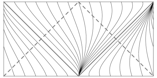
Figure 3: Conformal diagram of 1+1 dS spacetime with the flow lines of the aether field. Horizontal lines at the top and bottom represent null infinity, while the two vertical lines at left and right are identified. The solid and dashed grey lines form the past and future horizons of the Killing horizon for the boost symmetry under which the aether is invariant. The slope of the flow lines is $-\beta^{-1/2}$ on all boundaries of the diagram which is drawn for the case $\beta=0.1$.

The aether is regular in the planar coordinate system, which covers the triangle with solid grey edges. On these edges $u^{a}$ becomes infinitely stretched as it approaches a null direction. The solid grey lines form the past horizon part of the Killing horizon for the boost symmetry under which the aether is invariant, while the dashed grey lines form the future horizon part. The aether cannot possibly be regular at the bifurcation points where the past and future horizons intersect, since these are fixed points of the Killing flow hence a unit timelike vector cannot be invariant there. (A similar circumstance occurs in the context of the 3+1 dimensional black hole solutions in Einstein-aether theory Eling:2004dk ; Eling:2006ec .) However, the aether is regular on the horizon to the future of the bifurcation points. This solution therefore provides a setting with a nonsingular aether flowing across a future horizon.

IV.2.4 $\beta>1$: Anti-de Sitter solution

When $\beta>1$ the curvature scalar (51) is positive, hence (with our signature choice) the constant curvature solutions for this theory correspond to anti-de Sitter space. In two dimensions dS and AdS are exactly the same spacetime locally, only with a reversal in the identification of what are the timelike and spacelike directions. Rather than going through the details we simply remark here that the aether solution for the AdS case can be obtained from the dS case by interchanging the planar $t$ and $x$ coordinates. This leads to the AdS metric in Poincaré coordinates, covering the so-called “Poincaré patch”, and to the $u^{a}$ field appropriate to the AdS space. The flow lines of the aether are again given in the embedding coordinates by (63), only now with $\beta>1$. In Fig. 3 we plot this flow and the Killing horizons in a conformal diagram for AdS. To avoid closed timelike curves we can pass to the covering space as is usually done, in which case the diagram should be extended infinitely in the vertical direction.

V Discussion

In this paper we have shown that the general Einstein-aether action can be parameterized by two coupling constants in 1+1 dimensional spacetime, and the classical equations of motion depend only on one combination $\beta$ of these. Hence there is a one-parameter family of classical theories. Using a field redefinition of the metric, we demonstrated that for $\beta>0$ the theory can be reduced to a form involving only one coupling constant which does not affect the classical solutions. The only solutions to this reduced theory are a flat metric together with one of three distinct types of solutions for the aether field. Via the inverse field redefinition these produce all solutions for the the generic theory, namely (i) flat spacetime with constant aether, (ii) constant curvature spacetimes with a uniformly accelerated $u^{a}$ invariant under a two-dimensional symmetry group generated by a boost and a null rotation, and (iii) a non-constant curvature spacetime that has no Killing symmetries and contains singularities. The sign of the curvature is determined by whether the coupling $\beta$ is less or greater than one. For $\beta<0$ only the solutions (i) and (iii) are present.

Unlike in dilaton gravity, there are no asymptotically flat black hole solutions, although the de Sitter and anti-de Sitter solutions possess Killing horizons that could allow issues of black hole thermodynamics to be studied. This classical study of the behavior of Einstein-aether theory in 1+1 dimensions may provide a starting point for further investigations into semiclassical and fully quantum toy models of quantum gravity with a dynamical preferred frame.

References

- (1) C. Teitelboim, “Gravitation and hamiltonian structure in two space-time dimensions,” Phys. Lett. B 126, 41 (1983); R. Jackiw, “Liouville field theory: a two-dimensional model for gravity?”, in Quantum Theory of Gravity, ed. S. Christensen (Hilger, Bristol, 1984).
- (2) D. Grumiller, W. Kummer and D. V. Vassilevich, “Dilaton gravity in two dimensions,” Phys. Rept. 369, 327 (2002) [arXiv:hep-th/0204253].
- (3) J. D. Brown, M. Henneaux and C. Teitelboim, “Black holes in two space-time dimensions,” Phys. Rev. D 33, 319 (1986).
- (4) V. P. Frolov, “Two-dimensional black hole physics,” Phys. Rev. D 46, 5383 (1992).
- (5) C. G. Callan, S. B. Giddings, J. A. Harvey and A. Strominger, “Evanescent black holes,” Phys. Rev. D 45, 1005 (1992) [arXiv:hep-th/9111056].
- (6) A. Achucarro and M. E. Ortiz, “Relating black holes in two-dimensions and three-dimensions,” Phys. Rev. D 48, 3600 (1993) [arXiv:hep-th/9304068].
- (7) C. Eling, T. Jacobson and D. Mattingly, “Einstein-aether theory,” in Deserfest, eds. J. Liu, M. J. Duff, K. Stelle, and R. P. Woodard (World Scientific, 2006) [arXiv:gr-qc/0410001].
- (8) C. Eling and T. Jacobson, “Spherical solutions in Einstein-aether theory: static aether and stars,” arXiv:gr-qc/0603058, Class. Quant. Grav. to appear.
- (9) A. Einstein, “Spielen Gravitationsfelder im Aufbau der materiellen Elementarteilchen eine wesentliche Rolle?,” Sitzungsberichte der Koniglich Preussischen Akad. d. Wissenschaften, 349-356 (1919); translated as “Do gravitational fields play an essential part in the structure of the elementary particles of matter?,” in The Principle of Relativity, by A. Einstein et. al. (Dover, New York, 1952); J. L. Anderson and D. Finkelstein, “Cosmological constant and fundamental length,” Am. J. Phys. 39, 901 (1971); see also S. Weinberg, “The cosmological constant problem,” Rev. Mod. Phys. 61, 1 (1989), and references therein.
- (10) B. Z. Foster, “Metric redefinitions in Einstein-aether theory,” Phys. Rev. D 72, 044017 (2005) [arXiv:gr-qc/0502066].
- (11) M. Spradlin, A. Strominger and A. Volovich, “Les Houches lectures on de Sitter space,” arXiv:hep-th/0110007.
- (12) C. Eling and T. Jacobson, “Black holes in Einstein-aether theory,” arXiv:gr-qc/0604088, Class. Quant. Grav. to appear.