Towards absorbing outer boundaries in General Relativity

Abstract

We construct exact solutions to the Bianchi equations on a flat spacetime background. When the constraints are satisfied, these solutions represent in- and outgoing linearized gravitational radiation. We then consider the Bianchi equations on a subset of flat spacetime of the form $[0,T]\times B_{R}$, where $B_{R}$ is a ball of radius $R$, and analyze different kinds of boundary conditions on $\partial B_{R}$. Our main results are: i) We give an explicit analytic example showing that boundary conditions obtained from freezing the incoming characteristic fields to their initial values are not compatible with the constraints. ii) With the help of the exact solutions constructed, we determine the amount of artificial reflection of gravitational radiation from constraint-preserving boundary conditions which freeze the Weyl scalar $\Psi_{0}$ to its initial value. For monochromatic radiation with wave number $k$ and arbitrary angular momentum number $\ell\geq 2$, the amount of reflection decays as $(kR)^{-4}$ for large $kR$. iii) For each $L\geq 2$, we construct new local constraint-preserving boundary conditions which perfectly absorb linearized radiation with $\ell\leq L$. (iv) We generalize our analysis to a weakly curved background of mass $M$, and compute first order corrections in $M/R$ to the reflection coefficients for quadrupolar odd-parity radiation. For our new boundary condition with $L=2$, the reflection coefficient is smaller than the one for the freezing $\Psi_{0}$ boundary condition by a factor of $M/R$ for $kR>1.04$. Implications of these results for numerical simulations of binary black holes on finite domains are discussed.

I Introduction

A common approach for numerically solving the Einstein field equations on a spatially unbounded domain is to truncate the domain via an artificial boundary, thus forming a finite computational domain $\Omega$ with outer boundary $\partial\Omega$. In order to obtain a unique Cauchy evolution, it is necessary to impose boundary conditions at $\partial\Omega$. These boundary conditions should form a well posed initial boundary value problem (IBVP) and, ideally, be completely transparent to the physical problem on the unbounded domain. Short of achieving the ideal, one can try to develop so-called absorbing boundary conditions which form a well posed IBVP and insure that only a very small amount of spurious gravitational radiation is reflected from $\partial\Omega$ into the computational domain. Once the IBVP on $\Omega$ is formulated, it is solved via a numerical approximation scheme which, together with the truncation of the domain, introduces two artificial parameters: a discretization parameter $h$, describing the coarseness of the discretization, and a cut-off parameter $R$, which gives the size of the spatial domain $\Omega$. For a stable discretization, it is expected that the continuum solution of the unbounded problem is recovered in the limit where $h\to 0$ and $R\to\infty$. In practice, due to finite computer resources, it is not possible to take this limit. Instead, one needs to quantify how small $h$ and how large $R$ need to be so that the error is below a certain tolerance value.

In this article, we address the “$R$-dependent” part of this task. We analyze boundary conditions which have been recently presented in the literature, and provide estimates for the amount of spurious radiation coming from $\partial\Omega$. Additionally, we propose new boundary conditions for Einstein’s vacuum field equations which introduce significantly less reflections than existing conditions.

There has been a substantial amount of work on the construction of absorbing (also called non-reflecting in the literature) boundary conditions for wave problems in acoustics, electromagnetism, meteorology, and solid geophysics (see [1] for a review). One approach is based on a sequence of local boundary conditions [2, 3, 4] with increasing order of accuracy. Although higher order local boundary conditions usually involve solving a high order differential equation at the boundary, the problem can be dealt with by introducing auxiliary variables at the boundary surface [5, 6]. A different approach is based on fast converging series expansions of exact nonlocal boundary conditions (see [7] and references therein). Of particular interest for this article is the work by Lau [8, 9, 10], which generalizes the work in Ref. [7] to the construction of exact non-reflecting boundary conditions for the Regge-Wheeler and Zerilli equations, describing linear gravitational fluctuations about a Schwarzschild black hole. This approach is robust, very accurate, and stable. However, it is based on a detailed knowledge of the solutions which might not always be available in more general situations.

For the fully nonlinear Einstein equations, the construction of absorbing outer boundary conditions is particularly difficult. First of all, Einstein’s field equations determine the evolution of the metric tensor, so one does not know the geometrical structure of the spacetime before actually solving the IBVP. Hence, it is not clear a priori how the geometry of the outer boundary evolves. This poses a problem if one wants to fix, for example, the area of the boundary $\partial\Omega$ to its initial value. Second, in the Cauchy formulation of Einstein’s field equations, there exist constraint-violating modes which propagate with nontrivial characteristic speeds. This is in contrast to the standard Cauchy formulation of Maxwell’s equations, where the evolution equations imply that the constraint variables (namely, the divergence of the electric and magnetic fields) are constant in time. Since the constraint variables in General Relativity propagate non-trivially, constraint-preserving boundary conditions (CPBC) must be specified so that constraint violations are not introduced into the computational domain. Finally, in General Relativity, it is difficult to define precisely what is meant by outgoing and ingoing radiation. This is due to the nonlinear nature of the theory and its diffeomorphism invariance. (See Ref. [11] for a discussion of this problem for nonlinear gravitational plane waves.) These issues all contribute to the challenge of determining the amount of spurious reflections from the outer boundary.

A significant advance towards developing absorbing boundary conditions for General Relativity was the first (and, to date, the only) well posed IBVP for Einstein’s vacuum field equations presented in Ref. [12]. This work, which is based on a tetrad formulation, recasts the evolution equations into a first order symmetric hyperbolic form with maximally dissipative boundary conditions, for which (local in time) well posedness is guaranteed [13]. The boundary conditions constructed in [12] control part of the geometry of the boundary surface by specifying its constant mean curvature, control the radiation by prescribing suitable combinations of the complex Newman-Penrose scalars $\Psi_{0}$ and $\Psi_{4}$, where the null tetrad is constructed from the evolution vector field and the normal to the boundary, and are constraint-preserving. Recently, there has been considerable effort to generalize the work in Ref. [12] by specifying CPBC for the more commonly used metric formulations of gravity (see Refs. [14, 15, 16, 17, 18, 19, 20, 21] and references therein). In particular, the methods in Refs. [17, 16, 19, 18, 21] in addition to preserving the constraints, regulate the dynamical degrees of freedom by freezing the Newman-Penrose scalar $\Psi_{0}$, defined with respect to a suitably chosen null tetrad, to its initial value.

Work focused on eliminating reflections from the outer boundary during fully relativistic vacuum simulations has been performed by several authors. In Ref. [22], boundary conditions based on the work in Ref. [3], which are perfectly absorbing for quadrupolar solutions of the flat wave equation, are numerically implemented via spectral methods, and used in a constrained evolution scheme of Einstein’s field equations [23]. In Refs. [24, 25], solutions of the full nonlinear Einstein equations on a finite computational domain are matched to exact analytic, purely outgoing solutions of the weak field equations at the outer boundary of the domain. Refs. [26, 27, 28, 29] generalize this idea by matching the nonlinear equations to an “outer module”, a code in which the equations are linearized about a Schwarzschild background, in order to carry the waveforms far into the wave zone. However, at the interface where the matching occurs, the methods in Refs. [24, 25, 26, 27, 28] do not take into account either the constraints of the nonlinear Cauchy code or the characteristic structure of the nonlinear evolution equations, so it is not clear if the resulting problem is well posed (the work in [29], on the other hand, does take into account the constraints and the characteristic fields of the Cauchy code, and gives an implementation for the spherically symmetric Einstein equations coupled to a massless scalar field). Two other approaches presented in the literature for constructing absorbing boundary conditions are: matching the nonlinear Cauchy code to a nonlinear characteristic code (see Ref. [30] for a review and [31] for recent work) and matching an incoming characteristic formulation to an outgoing one at a time-like cylinder [32]. Finally, methods that avoid introducing an artificial outer boundary altogether compactify spatial infinity [33, 34], or make use of hyperboloidal slices and compactify null infinity (see, for instance, [35, 36, 37]).

In this article, we take a step closer to the construction of absorbing boundary conditions in General Relativity. In order to do so, the IBVP of Einstein’s field equations is analyzed on a compact domain $\Omega\subset\mathbb{R}^{3}$ with smooth outer boundary $\partial\Omega$ and two simplifying assumptions. The first assumption is that at all times, the boundary surface $\partial\Omega$ is far from the strong field region, so that the gravitational field near the outer boundary is weak. As a consequence, the field equations can be linearized to a first approximation about flat spacetime in the vicinity of the outer boundary. The linearized field equations can be conveniently described by the Bianchi equations, which yield a Lorentz-invariant system for the linearized Weyl tensor having a structure which is very similar to that of Maxwell’s equations. Moreover, the linearized Weyl tensor is invariant with respect to infinitesimal coordinate transformations, since it vanishes on the background [38], so there are no gauge modes. The second assumption is that the boundary $\partial\Omega$ is approximately a metric sphere of area $4\pi R^{2}$. This assumption is quite natural. In fact, modern numerical relativity codes based on multi-block finite differencing [39, 40, 41] or pseudo-spectral methods [42, 23] are designed to handle spherical outer boundaries.

Under these assumptions, it is sufficient to analyze the Bianchi equations on a domain $\Omega=B_{R}$ consisting of a ball of radius $R$. We can then conveniently expand the linearized Weyl tensor in terms of spherical tensor harmonics, because of the spherical symmetry of $B_{R}$. The resulting equations are decoupled: they are a family of partial differential equations in one spatial dimension parameterized by the angular momentum numbers $\ell$ and $m$. For each fixed $\ell$ and $m$, the purely dynamical degrees of freedom can be described by a master equation for the Newman-Penrose scalar $\Psi_{2}$. This equation admits exact solutions which propagate along either in- or outgoing null radial geodesics. The in- and outgoing solutions are related to each other by a time reversal symmetry $t\mapsto-t$, making it possible to define sensibly in- and outgoing gravitational radiation. Hence, in our setting, it is clear how to quantify the amount of spurious radiation reflected at $\partial B_{R}$. Using these exact solutions, we analyze the quality of boundary conditions which have been proposed in the literature; namely, those which freeze all the incoming characteristic fields to their initial values, and CPBC which freeze the Weyl scalar $\Psi_{0}$ to its initial value. Furthermore, we offer a set of improved CPBC, which are perfectly absorbing for linearized radiation on a Minkowski background up to some arbitrary multipole number $\ell$. Finally, we extend our analysis to a weakly curved background.

Our main results are the following. First, we show that the naive boundary condition which freezes all the incoming characteristic fields to their initial values is not compatible with the constraints. To show this, we construct explicit solutions to the IBVP which have the property that they satisfy the constraints exactly on the initial time slice $t=0$, but violate them at later times $t>0$. Second, we impose CPBC and freeze the Weyl scalar $\Psi_{0}$ at the boundary to its initial value. The exact outgoing solutions do not satisfy this boundary condition exactly. Specifically, the quantity $\Psi_{0}$ constructed from these solutions falls off as $1/r^{5}$ along the null geodesics $t=r+{\text{c}onst.}$, where $r$ denotes the areal radius coordinate. This means that a solution to the IBVP corresponding to the boundary condition $\partial_{t}\Psi_{0}=0$ consists of a superposition of an in- and an outgoing wave, where the magnitude of the ratio of the ingoing to the outgoing wave amplitudes (which we define as the reflection coefficient) measures the amount of spurious reflection. We find that for monochromatic radiation with wave number $k$ and arbitrary angular momentum number $\ell\geq 2$, the reflection coefficient decays as $(kR)^{-4}$ for large $kR$. In particular, the reflection coefficient lies below $0.1\%$ for quadrupolar radiation with $kR\geq 6.4$. Third, for each $L\geq 1$, we construct local CPBC ${\cal B}_{L}$ which, for $L\geq 2$, improve the CPBC involving $\partial_{t}\Psi_{0}=0$, being perfectly absorbing for linearized gravitational radiation on Minkowski space with angular momentum number $\ell\leq L$. (${\cal B}_{1}$ is just the freezing $\Psi_{0}$ boundary condition and there is no improvement.) Since in many practical situations one expects the few lower multipoles to dominate, an implementation of ${\cal B}_{L}$ for $L=2$, $3$, or $4$ should result in only a small amount of spurious reflection. For $L=2$, our improved boundary condition ${\cal B}_{2}$ reads

$$\partial_{t}\left.(\partial_{t}+\partial_{r})(r^{5}\Psi_{0})\right|_{r=R}=0.$$ (1)

Finally, we take into account first order corrections from the curvature of the background. Since we assume that the outer boundary lies in the weak field regime, we describe spacetime near the outer boundary by a perturbed Schwarzschild metric of mass $M$, thereby generalizing our previous analysis by taking into account curvature near the outer boundary. To estimate the effects due to curvature, we compute the first order corrections in $2M/R$ to the exact in- and outgoing solutions with $\ell=2$ and odd parity, and then recalculate our reflection coefficient for the CPBC involving $\partial_{t}\Psi_{0}=0$. We find that for $2M/R\ll 1$, the corrected $\ell=2$ odd-parity reflection coefficient depends only weakly on $2M/R$. In fact, our results indicate that the reflection coefficient even decreases when $2M/R$ increases (but stays small). For quadrupolar solutions satisfying the improved boundary condition (1), which is perfectly absorbing for $M=0$, we find that the reflection coefficient decays as $(2M/R)(kR)^{-4}$ for large $kR$ and small $2M/R$. More precisely, the reflection coefficient is less than the one for the freezing $\Psi_{0}$ boundary condition by a factor of $M/R$ for $kR>1.04$.

This work is organized as follows. In Sect. II, we write down the Bianchi equations on an arbitrary spacetime. These equations can be obtained from the Bianchi identities after imposing the Einstein field equations. Next, we assume the existence of a spacelike foliation and a preferred radial direction in each timeslice and perform a $2+1+1$ split of the Bianchi equations, which separate into evolution and constraint equations. The constraint propagation system describing the evolution of constraint errors is also discussed.

In Sect. III, we specialize to a flat spacetime background of the form $[0,T]\times B_{R}$, where $B_{R}$ denotes a ball of radius $R$. By performing a decomposition into spherical tensor harmonics with angular momentum number $\ell$, we show that for each $\ell\geq 2$, the Bianchi equations can be reduced to two master equations. The first master equation describes the propagation of constraint violations, and is homogeneous. The second is an equation for $\Psi_{2}$, describing the propagation of linearized gravitational radiation, and has a source term which depends on the solution of the first master equation. One of the advantages of working with a master equation for $\Psi_{2}$ instead of a master equation for $\Psi_{0}$ or $\Psi_{4}$, as is usually done when studying perturbations of black holes with a Petrov type D metric [43, 44], is that for linearization about Minkowski spacetime, the former is invariant with respect to time reversal. Consequently, there is a nice symmetry between in- and outgoing solutions: one can be obtained from the other by changing the sign of $t$. This symmetry makes it possible to define the reflection coefficients in a natural way. In contrast, under time reversal, $\Psi_{0}$ is mapped to conjugate $\Psi_{4}$ and vice versa, so that the in- and outgoing parts of $\Psi_{0}$ look quite different. It is shown in this section that the master equations governing the constraint violations and the gravitational radiation both admit exact analytical solutions, which can be obtained by applying suitable differential operators to the solution of the one-dimensional flat wave equation. These solutions can be split in a unique way into in- and outgoing solutions describing, respectively, in- and outgoing constraint violations or in- and outgoing gravitational radiation.

In Sect. IV, we use the exact in- and outgoing solutions found in the previous section to construct exact solutions to the IBVP on $B_{R}$ corresponding to different boundary conditions on $\partial B_{R}$. In Sect. IV.1, we start by analyzing the characteristic structure of the evolution equations, and specify boundary conditions which freeze the incoming fields to their initial values. The incoming fields are related to the Weyl scalars $\Psi_{0}$ and $\Psi_{1}$, so these boundary conditions freeze $\Psi_{0}$ and $\Psi_{1}$ at the outer boundary to their initial values. By constructing an explicit solution with constraint satisfying data at $t=0$, we show that these “freezing” boundary conditions are not compatible with the constraints in the sense that the solution violates the constraints for $t>0$. Next, in Sect. IV.2, we replace the boundary condition which freezes $\Psi_{1}$ to its initial value with CPBC which guarantee that solutions of the IBVP satisfy the constraints everywhere on $B_{R}$ and at all times $t>0$, provided they hold initially. This can be achieved in two ways. The first is the one proposed in Ref. [12], which adds suitable combinations of the constraint equations to the evolution equations so that at the boundary, the constraints propagate tangentially to the boundary. The second is to analyze the characteristic structure of the constraint propagation system, and set the incoming constraint fields to zero at the boundary. Assuming in what follows that the constraints are satisfied exactly, we consider only the homogeneous master equation for $\Psi_{2}$. We impose the freezing boundary condition $\partial_{t}\Psi_{0}=0$ at the boundary $r=R$ on a superposition of in- and outgoing monochromatic waves for arbitrary $\ell$, and calculate the resulting reflection coefficients. These coefficients, which depend only on the dimensionless quantity $kR$ (where $k$ is the wave number) are of order unity if $kR<\ell$, and decay as $(kR)^{-4}$ for large $kR$. In Sect. IV.3, we construct the hierarchy ${\cal B}_{1}$, ${\cal B}_{2}$,… of improved boundary conditions, having the property that ${\cal B}_{L}$ is perfectly absorbing for all linearized gravitational waves with angular momentum number $\ell$ up to and including $L$. The construction of these boundary conditions is strongly related to the hierarchy proposed in [3].

Finally, in Sect. V, we generalize our analysis to odd-parity perturbations of a Schwarzschild background of mass $M$. Assuming that $M/R\ll 1$, we compute first order corrections in $M/R$ to the reflection coefficient corresponding to the freezing $\Psi_{0}$ boundary condition, for $\ell=2$. In addition, we compute the reflection coefficient for the boundary condition ${\cal B}_{2}$ (which is perfectly absorbing for $M=0$), and show that it is smaller than the one for the freezing $\Psi_{0}$ condition by a factor of $M/R$ for $kR>1.04$.

Implications for the modeling of isolated systems such as a binary black holes are discussed in the conclusions. In an appendix, we show that the IBVP corresponding to the master equation for $\Psi_{2}$ and our new boundary conditions ${\cal B}_{2}$, ${\cal B}_{3}$,… is stable in the sense that the solutions depend uniquely and continuously on the initial data.

II The Bianchi identities

We consider the Bianchi equations

$$\nabla_{a}C^{a}{}_{bcd}=J_{bcd}\;$$ (2)

on a given background geometry $(M,g_{ab})$, with $C_{abcd}$ a tensor field possessing the same algebraic symmetries as the Weyl tensor:

$$C_{[abc]d}=0,\qquad C_{[ab][cd]}=C_{abcd}=C_{cdab}\,,\qquad g^{bd}C_{abcd}=0,$$ (3)

and $J_{bcd}$ a given source tensor which is traceless and satisfies $J_{[bcd]}=J_{b[cd]}=J_{bcd}$. Eq. (2) has its origin in the Bianchi identities,

$$\nabla_{a}W^{a}{}_{bcd}=\nabla_{[c}\left(G_{d]b}-\frac{1}{3}g_{d]b}g^{ef}G_{ef}\right),$$ (4)

where $W_{abcd}$ and $G_{ab}$ denote, respectively, the Weyl tensor and the Einstein tensor belonging to the metric $g_{ab}$. If Einstein’s equations are imposed, then the right-hand side of the identity (4) can be re-expressed in terms of the stress-energy tensor, and (4) becomes an equation for the Weyl tensor which is of the form of Eq. (2). The identity

$$\nabla_{a}\nabla_{b}C^{ab}{}_{cd}=C^{ab}{}_{e[c}R^{e}{}_{d]ab}\;,$$

where $R_{abcd}$ denotes the Riemann tensor belonging to the background metric $g_{ab}$, yields the integrability condition

$$\nabla^{b}J_{bcd}=C^{ab}{}_{e[c}R^{e}{}_{d]ab}\;.$$ (5)

The right-hand side of this equation vanishes if $g_{ab}$ is flat or conformally flat.

In Sections III and IV we will assume that the background geometry $(M,g_{ab})$ is flat, in which case Eq. (2) describes the propagation of linearized gravitational radiation, with $C_{abcd}$ the linearized Weyl tensor. Since the Weyl tensor vanishes for flat spacetime, $C_{abcd}$ is invariant with respect to infinitesimal coordinate transformations [38]. As a consequence, the Bianchi equations are well-suited for studying linearized gravitational waves since they are manifestly gauge-invariant. For a flat background geometry, the integrability condition (5) reduces to the requirement that $J_{bcd}$ be divergence-free.

Finally, the Bianchi equations (2) can be coupled either to equations for metric components and Christoffel symbols, or to equations for tetrad fields and connection coefficients, giving the full nonlinear vacuum Einstein equations [45, 46, 47, 12, 48].

II.1 $3+1$ split

We assume there exists a globally defined time function $t:M\to\mathbb{R}$ such that $M$ is foliated by spacelike hypersurfaces $\Sigma_{\tau}=\{p\in M:t(p)=\tau\}$. Let $n_{a}=-\alpha\nabla_{a}t$ be the future-directed unit normal to these slices, where the time orientation is chosen so that the lapse function, $\alpha$, is strictly positive. The three-metric $h_{ab}$ and extrinsic curvature $k_{ab}$ are defined as

$$h_{ab}\equiv g_{ab}+n_{a}n_{b}\;,\qquad k_{ab}\equiv\nabla_{a}n_{b}+n_{a}a_{b}\;,$$

where $a_{b}\equiv n^{a}\nabla_{a}n_{b}$ is the acceleration along the integral curves of $n_{a}$. For a one-form $v_{a}$ tangential to $\Sigma_{\tau}$ in the sense that $v_{a}n^{a}=0$, the spatial covariant derivative $D_{a}v_{b}$ is defined as $D_{a}v_{b}\equiv h_{a}{}^{c}h_{b}{}^{d}\nabla_{c}v_{d}$. The spatial covariant derivative of a general tangential tensor field is defined similarly. The electric and magnetic parts of $C_{abcd}$ are, respectively,

$$E_{ab}=C_{acbd}n^{c}n^{d},\qquad H_{ab}=\frac{1}{2}n^{c}C_{caef}\varepsilon^{ef}{}_{b}\;,$$

where $\varepsilon_{bcd}=n^{a}\varepsilon_{abcd}$ denotes the natural volume element on $(\Sigma_{t},h_{ab})$. From the symmetries (3) of $C_{abcd}$, it follows that $E_{ab}$ and $H_{ab}$ are symmetric, traceless, and orthogonal to $n^{a}$. Furthermore, the ten fields $\{E_{ab}$, $H_{ab}\}$ uniquely determine $C_{abcd}$:

$$C_{abcd}=-4n_{[a}E_{b][c}n_{d]}-\varepsilon_{ab}{}^{e}E_{ef}\varepsilon^{f}{}_{cd}-2n_{[a}H_{b]e}\varepsilon^{e}{}_{cd}+2\varepsilon_{ab}{}^{e}H_{e[c}n_{d]}\,.$$

The decomposition of Eq. (2) into components normal and tangential to $n^{a}$ yields the evolution equations

$$\pounds_{n}E_{ab} = -\varepsilon_{cd(a}(D^{c}+2a^{c})H^{d}{}_{b)}+5k_{(a}{}^{d}E_{b)d}-2kE_{ab}-h_{ab}k^{cd}E_{cd}+R_{ab}\;,$$ (6)

$$\pounds_{n}H_{ab} = +\varepsilon_{cd(a}(D^{c}+2a^{c})E^{d}{}_{b)}+5k_{(a}{}^{d}H_{b)d}-2kH_{ab}-h_{ab}k^{cd}H_{cd}+S_{ab}\;,$$ (7)

and the constraint equations

$$D^{b}E_{ab}-k^{cd}\varepsilon^{b}{}_{da}H_{cb} = P_{a}\;,$$ (8)

$$D^{b}H_{ab}+k^{cd}\varepsilon^{b}{}_{da}E_{cb} = Q_{a}\;.$$ (9)

In these equations, $k\equiv h^{ab}k_{ab}$,

$$P_{c}=n^{b}n^{d}J_{bcd}\,,\qquad Q_{a}=-\frac{1}{2}\,n^{b}\varepsilon_{a}{}^{cd}J_{bcd}\,,$$

$$R_{ef}=-h_{(e}{}^{b}n^{c}h_{f)}{}^{d}J_{bcd}\,,\qquad S_{ef}=-\frac{1}{2}\,h_{(e}{}^{b}\varepsilon_{f)}{}^{cd}J_{bcd}\,,$$

and $\pounds_{n}$ denotes the Lie derivative with respect to the unit normal field $n^{a}$. Notice that Eqs. (6,7) and (8,9) obey the “Dirac duality” symmetry

$$(E_{ab},H_{ab})\mapsto(H_{ab},-E_{ab}),\qquad(P_{a},Q_{a})\mapsto(Q_{a},-P_{a}),\qquad(R_{ab},S_{ab})\mapsto(S_{ab},-R_{ab}).$$ (10)

II.2 $2+1$ split

In addition to the foliation $\Sigma_{\tau}$ by spacelike hypersurfaces, the existence of a unit spatial vector field $s^{a}$ which is everywhere tangential to the hypersurfaces $\Sigma_{t}$ is assumed. The existence of such a vector field allows us to introduce a Newman-Penrose null tetrad

$$l^{a}=\frac{1}{\sqrt{2}}\left(n^{a}+s^{a}\right),\qquad k^{a}=\frac{1}{\sqrt{2}}\left(n^{a}-s^{a}\right),\qquad m^{a}=\frac{1}{\sqrt{2}}\left(v^{a}+i\,w^{a}\right),\qquad\bar{m}^{a}=\frac{1}{\sqrt{2}}\left(v^{a}-i\,w^{a}\right),$$

where $v^{a}$ and $w^{a}$ are two mutually orthogonal unit vector fields which are normal to $n^{a}$ and $s^{a}$. The corresponding Newman-Penrose Weyl scalars [49] are defined as

$$\Psi_{0} = C_{abcd}l^{a}m^{b}l^{c}m^{d},$$

$$\Psi_{1} = C_{abcd}l^{a}k^{b}l^{c}m^{d},$$

$$\Psi_{2} = C_{abcd}l^{a}m^{b}\bar{m}^{c}k^{d},$$

$$\Psi_{3} = C_{abcd}l^{a}k^{b}k^{c}\bar{m}^{d},$$

$$\Psi_{4} = C_{abcd}k^{a}\bar{m}^{b}k^{c}\bar{m}^{d}.$$

Next, we decompose $E_{ab}$ and $H_{ab}$ into components parallel and normal to $s_{a}$. More precisely, we write

$$E_{ab} = \left(s_{a}s_{b}-\frac{1}{2}\gamma_{ab}\right)\bar{E}+2s_{(a}\bar{E}_{b)}+\hat{E}_{ab}\;,$$

$$H_{ab} = \left(s_{a}s_{b}-\frac{1}{2}\gamma_{ab}\right)\bar{H}+2s_{(a}\bar{H}_{b)}+\hat{H}_{ab}\;,$$

where $\gamma_{ab}=h_{ab}-s_{a}s_{b}$, $\bar{E}=E_{ab}s^{a}s^{b}$, $\bar{E}_{a}=\gamma_{a}{}^{b}E_{bc}s^{c}$, and $\hat{E}_{ab}=\left(\gamma_{a}{}^{c}\gamma_{b}{}^{d}-\frac{1}{2}\gamma_{ab}\gamma^{cd}\right)E_{cd}$ (with similar expressions for $\bar{H}$, $\bar{H}_{a}$ and $\hat{H}_{ab}$). In terms of these quantities, the Weyl scalars are

$$\Psi_{0} = \left[\hat{E}_{ab}+\varepsilon_{a}{}^{c}\hat{H}_{cb}\right]m^{a}m^{b},$$ (11)

$$\Psi_{1} = -\frac{1}{\sqrt{2}}\left[\bar{E}_{a}+\varepsilon_{a}{}^{b}\bar{H}_{b}\right]m^{a},$$ (12)

$$\Psi_{2} = \frac{1}{2}\left[\bar{E}-i\bar{H}\right],$$ (13)

$$\Psi_{3} = -\frac{1}{\sqrt{2}}\left[\bar{E}_{a}-\varepsilon_{a}{}^{b}\bar{H}_{b}\right]\bar{m}^{a},$$ (14)

$$\Psi_{4} = \left[\hat{E}_{ab}-\varepsilon_{a}{}^{c}\hat{H}_{cb}\right]\bar{m}^{a}\bar{m}^{b},$$ (15)

where $\varepsilon_{ab}=\varepsilon_{abc}s^{c}$.

In order to decompose the evolution equations (6,7), we make additional assumptions on the vector fields $n^{a}$ and $s^{a}$. First, we assume that $s^{a}$ is geodetic and everywhere orthogonal to closed $2$-surfaces $S_{r}$ in $\Sigma_{t}$. This implies that

$$D_{a}s_{b}=\kappa_{ab}\;,$$

where $\kappa_{ab}$ is a symmetric tensor field which is orthogonal to $s^{a}$, representing the extrinsic curvature of the $2$-surfaces $S_{r}$ as embedded in $\Sigma_{t}$. Next, we assume that the Lie-derivative $\pounds_{n}s^{a}$ of the vector field $s^{a}$ with respect to $n^{a}$ can be written as a linear combination of $n^{a}$ and $s^{a}$. This implies that any covariant tensor field $t_{a_{1}a_{2}...a_{k}}$ which is orthogonal to $n^{a}$ and $s^{a}$ has the property that $\pounds_{n}t_{a_{1}a_{2}...a_{k}}$ is again orthogonal to $n^{a}$ and $s^{a}$. Finally, we assume that the Lie-derivative $\pounds_{n}s_{a}$ of the one-form $s_{a}$ is proportional to $s_{a}$. These properties, together with the relations $n_{a}s^{a}=0$, $s_{a}s^{a}=1$, $\pounds_{n}n_{a}=D_{a}(\log\alpha)$, and $\pounds_{n}h_{ab}=2k_{ab}$, imply that

$$\bar{k}_{a}\equiv\gamma_{a}{}^{b}k_{bc}s^{c}=0,\qquad\pounds_{n}s^{a}=(\pounds_{s}\log\alpha)n^{a}-\bar{k}s^{a},\qquad\pounds_{n}s_{a}=\bar{k}s_{a}\;,$$

where $\bar{k}=k_{ab}s^{a}s^{b}$. Although these assumptions are strong, and may not all hold for a generic spacetime, they are satisfied for the background spacetimes and foliations used in this article. In particular, they are met for any spherically symmetric spacetime of the form

$$ds^{2}=-\alpha^{2}dt^{2}+\gamma^{2}\left(dr+\beta\,dt\right)^{2}+r^{2}\left(d\vartheta^{2}+\sin^{2}\vartheta\,d\varphi^{2}\right),$$

where $\alpha$, $\beta$ and $\gamma$ are smooth functions of $t$ and $r$, and where $n_{a}dx^{a}=-\alpha dt$ and $s_{a}dx^{a}=\gamma(dr+\beta dt)$. Decomposing the extrinsic curvature $k_{ab}$ as

$$k_{ab}=\left(s_{a}s_{b}-\frac{1}{2}\gamma_{ab}\right)\bar{k}+\hat{k}_{ab}+\frac{1}{2}\gamma_{ab}k,$$

where $\hat{k}_{ab}=\left(\gamma_{a}{}^{c}\gamma_{b}{}^{d}-\frac{1}{2}\gamma_{ab}\gamma^{cd}\right)k_{cd}$, we find from evolution equation (6) that

$$\pounds_{n}\bar{E} = -\frac{1}{\alpha^{2}}\varepsilon^{ab}{\cal D}_{a}\left(\alpha^{2}\bar{H}_{b}\right)+\hat{\kappa}^{ab}\varepsilon_{a}{}^{c}\hat{H}_{cb}+\frac{3}{2}\left(\bar{k}-k\right)\bar{E}-\hat{k}^{ab}\hat{E}_{ab}+\bar{R}\;,$$ (16)

$$\pounds_{n}\bar{E}_{a} = \frac{1}{2\alpha^{2}}\pounds_{s}\left(\alpha^{2}\varepsilon_{a}{}^{b}\bar{H}_{b}\right)-\frac{1}{2\alpha^{2}}{\cal D}^{c}\left(\alpha^{2}\varepsilon_{a}{}^{d}\hat{H}_{cd}\right)-\frac{3}{4\alpha^{2}}\varepsilon_{a}{}^{b}{\cal D}_{b}\left(\alpha^{2}\bar{H}\right)$$ (17)

$$- 2\hat{\kappa}_{a}{}^{b}\varepsilon_{b}{}^{c}\bar{H}_{c}+\frac{1}{4}\left(\bar{k}-3k\right)\bar{E}_{a}+\frac{5}{2}\hat{k}_{a}{}^{b}\bar{E}_{b}+\bar{R}_{a}\;,$$

$$\pounds_{n}\hat{E}_{ab} = \left[\frac{1}{\alpha^{2}}\pounds_{s}\left(\alpha^{2}\varepsilon_{a}{}^{c}\hat{H}_{bc}\right)+\frac{1}{\alpha^{2}}\varepsilon_{c(a}{\cal D}^{c}\left(\alpha^{2}\bar{H}_{b)}\right)-\left(3\hat{\kappa}_{c(a}+\frac{1}{2}\gamma_{c(a}\kappa\right)\varepsilon^{cd}\hat{H}_{b)d}-\frac{3}{2}\varepsilon_{(a}{}^{c}\hat{\kappa}_{b)c}\bar{H}\right]^{tf}$$ (18)

$$- \frac{1}{2}\left(5\bar{k}-k\right)\hat{E}_{ab}-\frac{3}{2}\hat{k}_{ab}\bar{E}+5\hat{k}_{(a}{}^{c}\hat{E}_{b)c}-\frac{3}{2}\gamma_{ab}\hat{k}^{cd}\hat{E}_{cd}+\hat{R}_{ab}\;,$$

where $[...]^{tf}$ denotes the trace-free part with respect to $\gamma_{ab}$, $\{\kappa$, $\hat{\kappa}_{ab}\}$ denote the trace and trace-free part of $\kappa_{ab}$, respectively, ${\cal D}$ denotes the covariant derivative compatible with $\gamma_{ab}$, and $\{\bar{R}$, $\bar{R}_{a}$, $\hat{R}_{ab}\}$ denote the parallel/parallel, parallel/transverse, and transverse trace-free parts of $R_{ab}$, respectively. The constraint equation (8) yields

$$\bar{P} = \pounds_{s}\bar{E}+{\cal D}^{a}\bar{E}_{a}-\hat{\kappa}^{ab}\hat{E}_{ab}+\frac{3\kappa}{2}\bar{E}+\hat{k}^{ab}\varepsilon_{a}{}^{c}\hat{H}_{bc}\;,$$ (19)

$$\bar{P}_{a} = \pounds_{s}\bar{E}_{a}+{\cal D}^{b}\hat{E}_{ab}-\frac{1}{2}{\cal D}_{a}\bar{E}+\kappa\bar{E}_{a}-\frac{1}{2}\left(3\bar{k}-k\right)\varepsilon_{a}{}^{b}\bar{H}_{b}-\hat{k}_{a}{}^{b}\varepsilon_{b}{}^{c}\bar{H}_{c}\;,$$ (20)

where we have defined $\bar{P}=P_{a}s^{a}$ and $\bar{P}_{a}=\gamma_{a}{}^{b}P_{b}$. Evolution and constraint equations for $\bar{H}$, $\bar{H}_{a}$ and $\hat{H}_{ab}$ are easily obtained by applying the Dirac duality transformations (10).

II.3 Propagation of the constraint fields

The decomposition of the integrability condition (5) into parts normal and tangential to $n^{a}$ gives (assuming that the background metric is flat or conformally flat)

$$\pounds_{n}P_{a} = -\frac{1}{2}\varepsilon_{a}^{\;\;cd}(D_{c}+3a_{c})Q_{d}+\frac{3}{2}\left(k_{a}{}^{b}P_{b}-kP_{a}\right)+(D^{b}+a^{b})R_{ab}+\varepsilon_{a}{}^{cd}k^{b}{}_{c}S_{bd}\,,$$ (21)

$$\pounds_{n}Q_{a} = \frac{1}{2}\varepsilon_{a}^{\;\;cd}(D_{c}+3a_{c})P_{d}+\frac{3}{2}\left(k_{a}{}^{b}Q_{b}-kQ_{a}\right)+(D^{b}+a^{b})S_{ab}-\varepsilon_{a}{}^{cd}k^{b}{}_{c}R_{bd}\,.$$ (22)

If the evolution equations (6,7) hold with $R_{ab}=S_{ab}=0$, then the fields $P_{a}$ and $Q_{a}$ obey homogeneous Maxwell-like equations with transmission speed half the speed of light. In particular, $P_{a}=Q_{a}=0$ on an initial spatial slice gives $P_{a}=Q_{a}=0$ on the future domain of dependence of the initial slice. We may therefore regard $P_{a}=Q_{a}=0$ as constraints which are propagated by the evolution equations (6,7) with $R_{ab}=S_{ab}=0$.

Under the same assumptions on the vector fields $n^{a}$ and $s^{a}$ as in the previous subsection, the $2+1$ split of the constraint propagation equations yields

$$\pounds_{n}\bar{P} = -\frac{1}{2\alpha^{3}}\varepsilon^{ab}{\cal D}_{a}\left(\alpha^{3}\bar{Q}_{b}\right)+\frac{1}{2}\left(\bar{k}-3k\right)\bar{P}$$ (23)

$$+ \frac{1}{\alpha}\pounds_{s}(\alpha\bar{R})+\frac{1}{\alpha}{\cal D}^{b}(\alpha\bar{R}_{b})-\hat{\kappa}^{ab}\hat{R}_{ab}+\frac{3\kappa}{2}\bar{R}+\hat{k}^{ab}\varepsilon_{a}{}^{c}\hat{S}_{bc}\;,$$

$$\pounds_{n}\bar{P}_{a} = \frac{1}{2\alpha^{3}}\varepsilon_{a}{}^{b}\left[\pounds_{s}(\alpha^{3}\bar{Q}_{b})-{\cal D}_{b}(\alpha^{3}\bar{Q})\right]-\frac{3}{4}\left(\bar{k}+k\right)\bar{P}_{a}+\frac{3}{2}\hat{k}_{a}{}^{b}\bar{P}_{b}$$ (24)

$$+ \frac{1}{\alpha}\pounds_{s}(\alpha\bar{R}_{a})+\frac{1}{\alpha}{\cal D}^{b}(\alpha\hat{R}_{ab})-\frac{1}{2\alpha}{\cal D}_{a}(\alpha\bar{R})+\kappa\bar{R}_{a}-\frac{1}{2}\left(3\bar{k}-k\right)\varepsilon_{a}{}^{b}\bar{S}_{b}-\hat{k}_{a}{}^{b}\varepsilon_{b}{}^{c}\bar{S}_{c}\;.$$

The corresponding equations for $\bar{Q}$ and $\bar{Q}_{a}$ are obtained from this by applying the Dirac duality transformations (10).

III Exact solutions on a Minkowski background

In this section, we consider the Bianchi equations (2) on the Minkowski background

$$ds^{2}=-dt^{2}+dr^{2}+r^{2}\hat{g}_{AB}dx^{A}dx^{B},$$

where $\hat{g}_{AB}dx^{A}dx^{B}=d\vartheta^{2}+\sin^{2}\vartheta\;d\varphi^{2}$ denotes the standard metric on $S^{2}$. A natural foliation is given by the slices $t=const.$, for which $n_{a}dx^{a}=-dt$, although other foliations are possible. (In particular, it should be interesting to generalize the investigation below to hyperboloidal slices.) Since the spacetime is spherically symmetric, it is natural to choose $s_{a}dx^{a}=dr$. The corresponding vector field $s^{a}$ is defined everywhere except at the center $r=0$. Furthermore, $\kappa=2/r$ and $\hat{\kappa}_{ab}=0$, so the evolution and constraint equations derived in the previous section simplify considerably. In this section, we assume that the source terms $R_{ab}$ and $S_{ab}$ vanish identically; however, we do not necessarily enforce the constraints $P_{a}=Q_{a}=0$ since we are also interested in studying the propagation of constraint violations.

III.1 Harmonic decomposition

Since the spacetime is spherically symmetric and the equations are linear, it is convenient to expand the fields in spherical tensor harmonics. In the resulting equations, pieces belonging to different angular momentum numbers $\ell$ and $m$ decouple. Thus, it is sufficient to consider one fixed value of $\ell$ and $m$ at a time. The decomposition of the fields $E_{ab}$ and $H_{ab}$ into spherical tensor harmonics reads

$$\bar{E} = \frac{1}{r}e_{0}(t,r)Y,$$

$$\bar{E}_{A} = e_{1}(t,r)\hat{\nabla}_{A}Y+f_{1}(t,r)\hat{S}_{A}\;,$$

$$\hat{E}_{AB} = 2re_{2}(t,r)\left[\hat{\nabla}_{A}\hat{\nabla}_{B}\right]^{tf}Y+2rf_{2}(t,r)\hat{\nabla}_{(A}\hat{S}_{B)}\;,$$ (25)

$$\bar{H} = \frac{1}{r}h_{0}(t,r)Y,$$

$$\bar{H}_{A} = h_{1}(t,r)\hat{\nabla}_{A}Y+g_{1}(t,r)\hat{S}_{A}\;,$$

$$\hat{H}_{AB} = 2rh_{2}(t,r)\left[\hat{\nabla}_{A}\hat{\nabla}_{B}\right]^{tf}Y+2rg_{2}(t,r)\hat{\nabla}_{(A}\hat{S}_{B)}\;,$$

where $Y=Y^{\ell m}(\vartheta,\varphi)$ denotes the standard spherical harmonics, $\hat{S}_{A}=\varepsilon_{A}{}^{B}\hat{\nabla}_{B}Y$, and $\hat{\nabla}$ denotes the covariant derivative on $S^{2}$. Similarly, the constraint variables can be written as

$$\bar{P}=\frac{1}{r}P_{0}(t,r)Y,\qquad\bar{P}_{A}=P_{1}(t,r)\hat{\nabla}_{A}Y+P_{2}(t,r)\hat{S}_{A}\;,$$ (26)

$$\bar{Q}=\frac{1}{r}Q_{0}(t,r)Y,\qquad\bar{Q}_{A}=Q_{1}(t,r)\hat{\nabla}_{A}Y+Q_{2}(t,r)\hat{S}_{A}\;.$$ (27)

The Newman-Penrose scalars are

$$\Psi_{0} = \frac{2}{r}(e_{2}-g_{2})\hat{m}^{A}\hat{m}^{B}\hat{\nabla}_{A}\hat{\nabla}_{B}Y+\frac{2}{r}(f_{2}+h_{2})\hat{m}^{A}\hat{m}^{B}\hat{\nabla}_{A}\hat{S}_{B}\;,$$ (28)

$$\Psi_{1} = -\frac{1}{\sqrt{2}r}(e_{1}-g_{1})\hat{m}^{A}\hat{\nabla}_{A}Y-\frac{1}{\sqrt{2}r}(f_{1}+h_{1})\hat{m}^{A}\hat{S}_{A}\;,$$ (29)

$$\Psi_{2} = \frac{1}{2r}\left(e_{0}-ih_{0}\right)Y,$$ (30)

$$\Psi_{3} = -\frac{1}{\sqrt{2}r}(e_{1}+g_{1})\bar{\hat{m}}^{A}\hat{\nabla}_{A}Y-\frac{1}{\sqrt{2}r}(f_{1}-h_{1})\bar{\hat{m}}^{A}\hat{S}_{A}\;,$$ (31)

$$\Psi_{4} = \frac{2}{r}(e_{2}+g_{2})\bar{\hat{m}}^{A}\bar{\hat{m}}^{B}\hat{\nabla}_{A}\hat{\nabla}_{B}Y+\frac{2}{r}(f_{2}-h_{2})\bar{\hat{m}}^{A}\bar{\hat{m}}^{B}\hat{\nabla}_{A}\hat{S}_{B}\;,$$ (32)

where $\hat{m}^{A}=r\,m^{A}$. Using the identities

$$\hat{\nabla}^{B}\left[\hat{\nabla}_{A}\hat{\nabla}_{B}\right]^{tf}Y = -\frac{\lambda}{2}\hat{\nabla}_{A}Y,$$ (33)

$$\hat{\nabla}^{B}\hat{\nabla}_{(A}\hat{S}_{B)} = -\frac{\lambda}{2}\hat{S}_{A}\;,$$ (34)

where $\lambda=(\ell-1)(\ell+2)$, the Bianchi equations yield a set of two decoupled systems for the amplitudes $(e_{0},e_{1},e_{2},g_{1},g_{2})$ (even parity sector) and $(h_{0},h_{1},h_{2},f_{1},f_{2})$ (odd-parity sector). For $\ell\geq 2$, the even parity sector is described by the evolution system

$$\dot{e}_{0} = -\frac{\ell(\ell+1)}{r}g_{1}\;,$$ (35)

$$\dot{e}_{1} = -\frac{1}{2}g_{1}^{\prime}-\frac{\lambda}{2r}g_{2}\;,$$ (36)

$$\dot{e}_{2} = -g_{2}^{\prime}+\frac{1}{2r}g_{1}\;,$$ (37)

$$\dot{g}_{1} = -\frac{1}{2}e_{1}^{\prime}-\frac{\lambda}{2r}e_{2}+\frac{3}{4r}e_{0}\;,$$ (38)

$$\dot{g}_{2} = -e_{2}^{\prime}+\frac{1}{2r}e_{1}\;,$$ (39)

where here and in the following, a dot and a prime denote differentiation with respect to $t$ and $r$, respectively. The evolution system (35,36,37,38,39) is subject to the constraints $P_{0}=P_{1}=Q_{2}=0$, where

$$P_{0} = \frac{1}{r^{2}}(r^{2}e_{0})^{\prime}-\frac{\ell(\ell+1)}{r}e_{1}\;,$$ (40)

$$P_{1} = \frac{1}{r^{2}}(r^{2}e_{1})^{\prime}-\frac{\lambda}{r}e_{2}-\frac{1}{2r}e_{0}\;,$$ (41)

$$Q_{2} = \frac{1}{r^{2}}(r^{2}g_{1})^{\prime}-\frac{\lambda}{r}g_{2}\;.$$ (42)

The odd-parity sector is obtained from this after the substitutions $(e_{0},e_{1},e_{2},g_{1},g_{2})\mapsto(h_{0},h_{1},h_{2},-f_{1},-f_{2})$. Therefore, it is sufficient to discuss the even parity sector, which is what we will do in the following.

III.2 Exact solutions

In this section, we discuss how to obtain exact analytic solutions to this constrained evolution system. We start with the special cases $\ell=0$ and $\ell=1$ which, as we will see, are non-radiative. For $\ell=0$, the only equations are $\dot{e}_{0}=0$ and $(r^{2}e_{0})^{\prime}=0$ which yield the solution

$$e_{0}=-\frac{2M}{r^{2}}\;,\qquad M=const.$$ (43)

For $\ell=1$, $\hat{E}_{AB}$ and $\hat{H}_{AB}$ vanish, and the evolution equations for $e_{2}$ and $g_{2}$, and the constraint equation $Q_{2}=0$, are void. Taking a time derivative of the constraint $P_{0}=0$, and eliminating $\dot{e}_{0}$ and $\dot{e}_{1}$ using the evolution equations, one obtains $g_{1}=c(t)/r^{2}$, where the function $c$ is independent of $r$. The insertion of this information back into the evolution equations for $e_{0}$ and $e_{1}$ gives $e_{0}=-2e_{1}+k(r)$ for a function $k$ which is independent of $t$. Substitution of these results into the evolution equation for $g_{1}$ and the constraint $P_{1}=0$ gives $c(t)=c_{2}t+c_{1}$, $k(r)=2c_{2}/r$ for some constants $c_{1}$ and $c_{2}$, and $e_{1}=c_{2}/(2r)+f(t)/r^{3}$ for a function $f$ which is independent of $r$. Finally, the insertion of all this into the evolution equation for $e_{0}$ yields $\dot{f}=c_{2}t+c_{1}$. Thus, one obtains the most general solution in the sector $\ell=1$:

$$e_{0}=\frac{c_{2}}{r}-\frac{c_{2}t^{2}+2c_{1}t+2c_{0}}{r^{3}}\;,\qquad e_{1}=\frac{c_{2}}{2r}+\frac{c_{2}t^{2}+2c_{1}t+2c_{0}}{2r^{3}}\;,\qquad g_{1}=\frac{c_{2}t+c_{1}}{r^{2}}\;.$$

If we demand that the solution be stationary, then the corresponding odd-parity solution is

$$h_{0}=\frac{6J}{r^{3}}\;,\qquad h_{1}=-\frac{3J}{r^{3}}\;,\qquad f_{1}=0,\qquad J=const.$$ (44)

With the normalization $Y^{(\ell=0)}=1$, $Y^{(\ell=1)}=\cos\vartheta$, Eqs. (43,44) yield the linearized Weyl tensor belonging to the linearized Kerr metric

$$-dt^{2}+dr^{2}+r^{2}\left(d\vartheta^{2}+\sin^{2}\vartheta\,d\varphi^{2}\right)+\frac{2M}{r}\left(dt^{2}+dr^{2}\right)-\frac{4J}{r}\,\sin^{2}\vartheta\,d\varphi dt,$$

where the linearization is performed about flat spacetime in the mass parameter $M$ and the angular momentum parameter $J$.

Next, we consider the cases with $\ell\geq 2$. We obtain two classes of solutions, one representing outgoing radiation and the other representing incoming radiation. If the constraints are satisfied, these solutions correspond to those presented in [50, 24, 51]. To solve the above constrained evolution system, we first derive the constraint propagation system, which describes the propagation of constraint violations under the flux defined by the evolution equations (6,7). The constraint propagation system can be obtained either by performing a multipolar decomposition of the evolution system (23,24) with $R_{ab}=S_{ab}=0$, or by taking a time derivative of Eqs. (40,41,42) and using the evolution equations (35,36,37,38,39). The result is

$$\dot{P}_{0} = -\frac{\ell(\ell+1)}{2r}\,Q_{2}\;,$$ (45)

$$\dot{P}_{1} = -\frac{1}{2}\,Q_{2}^{\prime}\;,$$ (46)

$$\dot{Q}_{2} = -\frac{1}{2}\left(P_{1}^{\prime}-\frac{1}{r}P_{0}\right).$$ (47)

Solutions to this system have the form

$$P_{0}=-\frac{\ell(\ell+1)}{2r}\,\pi+rh^{\prime}(r),\qquad P_{1}=-\frac{1}{2}\pi^{\prime}+h(r),\qquad Q_{2}=\dot{\pi},$$ (48)

where $h(r)$ is a function of $r$ only and where the function $\pi$ satisfies the master equation

$$\left[\frac{1}{c^{2}}\partial_{t}^{2}-\partial_{r}^{2}+\frac{\ell(\ell+1)}{r^{2}}\right]\pi(t,r)=0,$$ (49)

with $c=1/2$. Eq. (49) describes the evolution of constraint violations which propagate at half the speed of light. How to solve Eq. (49) will be explained below.

Once the constraint variables $P_{0}$, $P_{1}$ and $Q_{2}$ have been obtained, we proceed as follows. First, using Eqs. (40,41,42) we express $e_{1}$, $e_{2}$ and $g_{2}$ in terms of $e_{0}$ and $g_{1}$ and the constraint variables:

$$\ell(\ell+1)e_{1} = \frac{1}{r}\phi^{\prime}-rP_{0}\;,$$ (50)

$$\lambda e_{2} = \frac{1}{\ell(\ell+1)r}\left[r\phi^{\prime}-r^{3}P_{0}\right]^{\prime}-\frac{1}{2r^{2}}\phi-rP_{1}\;,$$ (51)

$$\lambda g_{2} = \frac{1}{r}(r^{2}g_{1})^{\prime}-rQ_{2}\;,$$ (52)

where we have set $\phi=r^{2}e_{0}$. Next, using these expressions in Eqs. (35) and (38), we obtain the following wave equation for $\phi$:

$$\left[\partial_{t}^{2}-\partial_{r}^{2}+\frac{\ell(\ell+1)}{r^{2}}\right]\phi(t,r)=S(t,r),$$ (53)

where the source term $S(t,r)$ depends on the constraint variables $\pi(t,r)$ and $h(r)$ and is given by

$$S(t,r)=\frac{\ell(\ell+1)}{4}\left[3r\pi^{\prime}+2\pi-2rh(r)\right]-[r^{3}h^{\prime}(r)]^{\prime}.$$

Once Eq. (53) has been solved for $\phi(t,r)$, the quantities $e_{1}$, $e_{2}$ and $g_{2}$ are obtained from Eqs. (50,51,52). Therefore, the linearized equations reduce to the two master equations (49,53).

We now discuss how to obtain exact solutions to these equations. We start with the homogeneous case where $S(t,r)=0$. For the following, it is convenient to introduce for each $\ell=0,1,2,...$ the operators [50]

$$a_{\ell}\equiv\partial_{r}+\frac{\ell}{r}=r^{-\ell}\partial_{r}(r^{\ell}.),$$

and their formal adjoints

$$a_{\ell}^{\dagger}\equiv-\partial_{r}+\frac{\ell}{r}=-r^{\ell}\partial_{r}(r^{-\ell}.).$$

They satisfy the operator identities

$$a_{\ell+1}a_{\ell+1}^{\dagger}=a_{\ell}^{\dagger}a_{\ell}=-\partial_{r}^{2}+\frac{\ell(\ell+1)}{r^{2}}\;.$$ (54)

As a consequence, for each $\ell=0,1,2,...$,

$$\left[\partial_{t}^{2}-\partial_{r}^{2}+\frac{\ell(\ell+1)}{r^{2}}\right]a_{\ell}^{\dagger}a_{\ell-1}^{\dagger}...a_{1}^{\dagger} = \left[\partial_{t}^{2}+a_{\ell}^{\dagger}a_{\ell}\right]a_{\ell}^{\dagger}a_{\ell-1}^{\dagger}...a_{1}^{\dagger}$$ (55)

$$= a_{\ell}^{\dagger}\left[\partial_{t}^{2}+a_{\ell-1}^{\dagger}a_{\ell-1}\right]a_{\ell-1}^{\dagger}...a_{1}^{\dagger}$$

$$= a_{\ell}^{\dagger}a_{\ell-1}^{\dagger}...a_{1}^{\dagger}\left[\partial_{t}^{2}-\partial_{r}^{2}\right].$$

Therefore, in- and outgoing solutions to the homogeneous master equation can be constructed from in- and outgoing solutions of the one-dimensional wave equation [50]. For $\ell=0$, the in- and outgoing solutions are given, respectively, by $\phi_{\nwarrow,0}(t,r)\equiv V_{0}(r+t)$ and $\phi_{\nearrow,0}(t,r)\equiv U_{0}(r-t)$, where $V_{0}$ and $U_{0}$ are smooth functions. For $\ell>0$ the solutions have the form

$$\phi_{\nwarrow,\ell}(t,r) = a_{\ell}^{\dagger}a_{\ell-1}^{\dagger}...a_{1}^{\dagger}V_{\ell}(r+t),$$

$$\phi_{\nearrow,\ell}(t,r) = a_{\ell}^{\dagger}a_{\ell-1}^{\dagger}...a_{1}^{\dagger}U_{\ell}(r-t),$$

where $V_{\ell}$ and $U_{\ell}$ are sufficiently smooth functions. Explicit expressions for $\phi_{\nwarrow,\ell}$ and $\phi_{\nearrow,\ell}$ are given by

$$\phi_{\nwarrow,\ell}(t,r) = (-1)^{\ell}r^{\ell}\left(\frac{d}{dr}\frac{1}{r}\right)^{\ell}V_{\ell}(r+t)=\sum\limits_{j=0}^{\ell}(-1)^{j}\frac{(2\ell-j)!}{(\ell-j)!\,j!}(2r)^{j-\ell}V^{(j)}_{\ell}(r+t),$$ (56)

$$\phi_{\nearrow,\ell}(t,r) = (-1)^{\ell}r^{\ell}\left(\frac{d}{dr}\frac{1}{r}\right)^{\ell}U_{\ell}(r-t)=\sum\limits_{j=0}^{\ell}(-1)^{j}\frac{(2\ell-j)!}{(\ell-j)!\,j!}(2r)^{j-\ell}U^{(j)}_{\ell}(r-t),$$ (57)

where here and in the following, for a function $F$ on the real line, $F^{(j)}$ denotes its $j$’th derivative. As an example, for $\ell=2$,

$$\phi_{\nearrow,2}(t,r)=\frac{3}{r^{2}}U_{2}(r-t)-\frac{3}{r}U^{(1)}_{2}(r-t)+U^{(2)}_{2}(r-t).$$

In- and outgoing solutions of the constraint propagation master equation (49) can be obtained in exactly the same way after replacing $t$ by $ct$, ie.,

$$\pi_{\nwarrow,\ell}(t,r) = a_{\ell}^{\dagger}a_{\ell-1}^{\dagger}...a_{1}^{\dagger}W_{\ell}(r+ct),$$

$$\pi_{\nearrow,\ell}(t,r) = a_{\ell}^{\dagger}a_{\ell-1}^{\dagger}...a_{1}^{\dagger}Z_{\ell}(r-ct),$$

for some sufficiently smooth functions $W_{\ell}$ and $Z_{\ell}$.

Finally, we discuss the case $S(t,r)\neq 0$. Since we have already calculated the solutions to the homogeneous problem, it is sufficient to construct one particular solution of Eq. (53). In the following, we assume that $h\equiv 0$ and that $\pi(t,r)$ has the form $\pi(t,r)=a_{\ell}^{\dagger}a_{\ell-1}^{\dagger}...a_{1}^{\dagger}W_{\ell}(t,r)$, with $W_{\ell}$ a sufficiently smooth function of $t$ and $r$. The latter assumption is no restriction of generality, since we can obtain $W_{\ell}$ from $\pi$ by successive integration,

$$W_{\ell}(t,r)=r\int\limits_{r}^{\infty}dr_{1}r_{1}\int\limits_{r_{1}}^{\infty}dr_{2}r_{2}...\int\limits_{r_{\ell-1}}^{\infty}dr_{\ell}\frac{\pi(t,r_{\ell})}{r_{\ell}^{\ell}}\;,$$

provided that $\pi(t,.)$ falls off sufficiently rapidly as $r\to\infty$. To construct a particular solution $\phi_{1}(t,r)$ of Eq. (53), we first notice that the operators

$$p_{m}=3r\partial_{r}+m,$$

$m=...-2,-1,0,1,2,...$ satisfy the commutation relations

$$p_{m}a_{\ell}^{\dagger}=a_{\ell}^{\dagger}p_{m-3}\;.$$

As a consequence,

$$S(t,r)=\frac{\ell(\ell+1)}{4}\,p_{2}\pi(t,r)=\frac{\ell(\ell+1)}{4}\,a_{\ell}^{\dagger}a_{\ell-1}^{\dagger}...a_{1}^{\dagger}p_{2-3\ell}W_{\ell}(t,r).$$

If we make the ansatz

$$\phi_{1}(t,r)=a_{\ell}^{\dagger}a_{\ell-1}^{\dagger}...a_{1}^{\dagger}\psi(t,r),$$

and use relation (55), we see that $\phi_{1}$ is a particular solution if $\psi$ satisfies the inhomogeneous one-dimensional wave equation

$$\left[\partial_{t}^{2}-\partial_{r}^{2}\right]\psi(t,r)=\frac{\ell(\ell+1)}{4}p_{2-3\ell}W_{\ell}(t,r).$$

With trivial initial data, this equation has the solution

$$\psi(t,r)=\frac{\ell(\ell+1)}{8}\int\limits_{0}^{t}\int\limits_{r-t+\tau}^{r+t-\tau}p_{2-3\ell}W_{\ell}(\tau,s)dsd\tau.$$

Therefore, a particular solution of Eq. (53) is given by

$$\phi_{1}(t,r)=\frac{\ell(\ell+1)}{8}a_{\ell}^{\dagger}a_{\ell-1}^{\dagger}...a_{1}^{\dagger}\int\limits_{0}^{t}\int\limits_{r-t+\tau}^{r+t-\tau}p_{2-3\ell}W_{\ell}(\tau,s)dsd\tau.$$ (59)

IV Solutions of the initial-boundary value problem

In this section, we analyze the Bianchi equations in the presence of artificial boundaries. Specifically, we solve the equations on a tubular subspace $M=[0,T]\times B_{R}$ of Minkowski spacetime, where $B_{R}$ is a ball of radius $R$ in Euclidean space. Our goal is to impose boundary conditions on the timelike boundary ${\cal T}=[0,T]\times\partial B_{R}$ which are perfectly absorbing in the following sense: for given initial data which is compactly supported in $B_{R}$ and which represents a purely outgoing solution, the solution to the IBVP leads to the same solution as the solution to the global problem (without artificial boundaries). As discussed in the introduction, this turns out to be a challenging problem, even for simpler systems like the wave equation in more than one dimension [2, 3]. The strategy here will be to impose different boundary conditions on ${\cal T}$ which have been proposed in the literature, and construct exact solutions of the resulting IBVP by using the expressions derived in the previous section. With the help of these solutions, we analyze how “good” the boundary conditions are by looking at the amount of artificial reflection of constraint violating modes and gravitational radiation. This analysis enables us to construct different classes of boundary conditions, where each new class yields an improvement over the old one.

We start in the next subsection with our crudest approximation for constructing outgoing boundary conditions, which consists of using the symmetric hyperbolic structure of the evolution equations (6,7) to freeze the incoming characteristic fields to their initial values. These boundary conditions yield a well posed IBVP. However, as we show, they introduce constraint-violating modes into the computational domain and therefore fail to be perfectly absorbing at a very fundamental level.

In subsection IV.2, first we specify CPBC which freeze the Weyl scalar $\Psi_{0}$ to its initial value. This is done either by using the method in [12], where suitable combinations of the constraints are added to the evolution equations, or by setting to zero the incoming constraint fields. Then, we show that the resulting boundary conditions introduce some reflections of (linearized) gravitational radiation. We quantify the amount of reflection by considering outgoing waves with wave number $k$ and computing the reflection coefficient as a function of the dimensionless quantity $kR$.

Finally, in subsection IV.3, we improve the boundary conditions considered in subsection IV.2. In particular, for each $L\geq 1$, we give CPBC which are perfectly absorbing for outgoing gravitational radiation with angular momentum number $\ell\leq L$.

IV.1 Freezing the incoming fields

Let $s_{a}$ be the unit outward normal one-form to the boundary $\partial B_{R}$. For a symmetric hyperbolic evolution system of the form

$${\cal A}^{a}(u)\frac{\partial}{\partial x^{a}}u={\cal F}(u),$$

with ${\cal A}^{0}(u)=1\!\!1$, the characteristic speeds and fields with respect to $s_{a}$ are defined, respectively, as the eigenvalues and projections of $u$ onto the corresponding eigenspaces of the matrix ${\cal A}^{a}(u)s_{a}$. For the evolution system (6,7), these are given by

$$\mu=-\beta^{a}s_{a}\;, \bar{E}=2\mbox{Re}\Psi_{2}\;,\qquad\bar{H}=-2\mbox{Im}\Psi_{2}\;,$$

$$\mu=-\frac{\alpha}{2}-\beta^{a}s_{a}\;, \bar{V}^{(-)}_{a}=\bar{E}_{a}+\varepsilon_{a}{}^{b}\bar{H}_{b}=-\sqrt{2}(\Psi_{1}\bar{m}_{a}+\bar{\Psi}_{1}m_{a}),$$

$$\mu=+\frac{\alpha}{2}-\beta^{a}s_{a}\;, \bar{V}^{(+)}_{a}=\bar{E}_{a}-\varepsilon_{a}{}^{b}\bar{H}_{b}=-\sqrt{2}(\Psi_{3}m_{a}+\bar{\Psi}_{3}\bar{m}_{a}),$$

$$\mu=-\alpha-\beta^{a}s_{a}\;, \hat{V}^{(-)}_{ab}=\hat{E}_{ab}+\varepsilon_{(a}{}^{c}\hat{H}_{b)c}=(\Psi_{0}\bar{m}_{a}\bar{m}_{b}+\bar{\Psi}_{0}m_{a}m_{b}),$$

$$\mu=+\alpha-\beta^{a}s_{a}\;, \hat{V}^{(+)}_{ab}=\hat{E}_{ab}-\varepsilon_{(a}{}^{c}\hat{H}_{b)c}=(\Psi_{4}m_{a}m_{b}+\bar{\Psi}_{4}\bar{m}_{a}\bar{m}_{b}),$$

where we use the same notation as in Sect. II.2, and where $\beta^{a}$ denotes the shift vector field. The ingoing fields are the ones with negative characteristic speeds $\mu$. One way to obtain a well posed IBVP is to freeze the ingoing fields to their initial values [13]. In our choice of coordinates, with $\alpha=1$ and $\beta^{a}=0$, this boundary condition is equivalent to imposing

$$\partial_{t}\Psi_{0}\;\hat{=}\;0,\qquad\partial_{t}\Psi_{1}\;\hat{=}\;0,$$

where here and in the following we use the notation $\;\hat{=}\;$ to denote equalities which hold on the boundary $\partial B_{R}$ only.

We analyze these boundary conditions using the harmonic decomposition of the previous section. As noted before, it is sufficient to consider the even parity sector. In view of Eqs. (28-32), we define the radial Weyl scalars $\psi_{0}\equiv 2(e_{2}-g_{2})$, $\psi_{1}\equiv e_{1}-g_{1}$, $\psi_{2}\equiv e_{0}$, $\psi_{3}\equiv e_{1}+g_{1}$, and $\psi_{4}\equiv 2(e_{2}+g_{2})$ which are functions of $t$ and $r$ only. Using the relations (35,50,51,52), the master equation (53), and Eq. (48), we find

$$\psi_{0} = \frac{b_{-}^{2}\phi}{(\ell-1)\ell(\ell+1)(\ell+2)r^{4}}+\frac{8r\dot{\pi}+5r\pi^{\prime}+6\pi}{4(\ell-1)(\ell+2)}\;,$$ (60)

$$\psi_{1} = \frac{b_{-}\phi}{\ell(\ell+1)r^{3}}+\frac{\pi}{2}\;,$$ (61)

$$\psi_{2} = \frac{\phi}{r^{2}}\;,$$ (62)

$$\psi_{3} = \frac{b_{+}\phi}{\ell(\ell+1)r^{3}}-\frac{\pi}{2}\;,$$ (63)

$$\psi_{4} = \frac{b_{+}^{2}\phi}{(\ell-1)\ell(\ell+1)(\ell+2)r^{4}}+\frac{-8r\dot{\pi}+5r\pi^{\prime}+6\pi}{4(\ell-1)(\ell+2)}\;,$$ (64)

where we have introduced the operators $b_{\pm}=r^{2}(\partial_{t}\mp\partial_{r})$ and again assumed that $h\equiv 0$ for simplicity. In what follows, the expressions

$$(b_{-})^{m}\phi_{\nwarrow,\ell}(t,r) = \frac{(\ell+m)!}{(\ell-m)!}\,r^{m}\sum\limits_{j=0}^{\ell+m}(-1)^{j+m}\frac{(2\ell-j)!}{(\ell+m-j)!\,j!}(2r)^{j-\ell}V^{(j)}_{\ell}(r+t),\qquad m=0,1,2,...\ell,$$ (65)

$$(b_{-})^{m}\phi_{\nwarrow,\ell}(t,r) = (-1)^{\ell}r^{m}\sum\limits_{j=0}^{m-\ell-1}\frac{(\ell+m)!}{(2\ell+1-j)!}\frac{(m-\ell-1)!}{(m-\ell-j-1)!\,j!}(2r)^{\ell+1+j}V^{(j)}_{\ell}(r+t),~{}m=\ell+1,\ell+2,...,$$ (66)

$$(b_{-})^{m}\phi_{\nearrow,\ell}(t,r) = r^{m}\sum\limits_{j=0}^{\ell-m}(-1)^{j+m}\frac{(2\ell-j)!}{(\ell-m-j)!\,j!}(2r)^{j-\ell}U^{(j)}_{\ell}(r-t),\qquad m=0,1,2...\ell,$$ (67)

$$(b_{-})^{m}\phi_{\nearrow,\ell}(t,r) = 0,\qquad m=\ell+1,\ell+2,...$$ (68)

will be useful. They can be derived from the explicit expressions (56,57) by induction in $m$. Corresponding expressions for $(b_{+})^{m}\phi$ can be obtained by flipping the sign of $t$ and interchanging $\phi_{\nwarrow,\ell}$ and $\phi_{\nearrow,\ell}$. We see from these expressions that if $\pi=0$ and $\phi=\phi_{\nearrow,\ell}$, then along the outgoing null rays $r-t=const.$, we have $b_{-}\phi=O(r^{0})$, $b_{-}^{2}\phi=O(r^{0})$ and $b_{+}\phi=O(r^{2})$, $b_{+}^{2}\phi=O(r^{4})$. Therefore, the radial Weyl scalars obey

$$\psi_{s}=O(r^{s-4}),\qquad r-t=const.$$ (69)

for $s=0,1,2,3,4$. This is consistent with the peeling theorem [52].

Next, we construct exact solutions of the IBVP described by the evolution equations (49,53), initial data for $\pi$ and $\phi$ on the interval $(0,R)$, and the boundary conditions $\partial_{t}\Psi_{0}\;\hat{=}\;\partial_{t}\Psi_{1}\;\hat{=}\;0$ imposed on a sphere of radius $R>0$. These solutions have the property of satisfying the constraints initially (ie. $\pi(0,r)=0$ and $\dot{\pi}(0,r)=0$ for all $0<r<R$), but violating the constraints at later times. For the sake of avoiding unnecessary complications, we restrict ourselves to the case $\ell=2$, although one should be able to construct similar solutions for higher $\ell$.

To construct these solutions, we start with a smooth function $F:(0,\infty)\to\mathbb{R}$ which is zero on the interval $(0,R)$ but non-zero for $r>R$, and set

$$\pi(t,r)=a_{2}^{\dagger}a_{1}^{\dagger}F^{(5)}(r+ct),$$

where $F^{(5)}$ denotes the fifth derivative of $F$. By construction, this solves the constraint master equation (49), and $\pi(0,r)=0$, $\dot{\pi}(0,r)=0$ for all $0<r<R$. Choosing $h\equiv 0$ guarantees that the constraint variables $P_{0}$, $P_{1}$ and $Q_{2}$ have trivial initial data as well. Next, using the construction procedure outlined in the previous section, we obtain the general solution of the inhomogeneous wave equation (53). The result is

$$\phi(t,r)=a_{2}^{\dagger}a_{1}^{\dagger}\left[\phi_{\nearrow}(r-t)+\phi_{\nwarrow}(r+t)+24F^{(3)}(r+ct)-6rF^{(4)}(r+ct)\right],$$ (70)

where $\phi_{\nearrow}$ and $\phi_{\nwarrow}$ are (up to this point) arbitrary smooth functions. In order to determine these functions, we insert the general solution (70) into the boundary conditions $\partial_{t}\Psi_{0}\;\hat{=}\;\partial_{t}\Psi_{1}\;\hat{=}\;0$. Using the expressions (60,61), we obtain

$$4r^{4}\psi_{0}(t,r) = \phi_{\nearrow}(r-t)+\phi_{\nwarrow}(r+t)-2r\phi^{(1)}_{\nwarrow}(r+t)+2r^{2}\phi^{(2)}_{\nwarrow}(r+t)-\frac{4}{3}\,r^{3}\phi^{(3)}_{\nwarrow}(r+t)+\frac{2}{3}\,r^{4}\phi^{(4)}_{\nwarrow}(r+t)$$ (71)

$$+ 4\left[6F^{(3)}(r+ct)-9rF^{(4)}(r+ct)+6r^{2}F^{(5)}(r+ct)-2r^{3}F^{(6)}(r+ct)\right],$$

$$-r^{4}\psi_{1}(t,r) = \phi_{\nearrow}(r-t)-\frac{1}{2}\,r\phi_{\nearrow}(r-t)+\phi_{\nwarrow}(r+t)-\frac{3}{2}\,r\phi^{(1)}_{\nwarrow}(r+t)+r^{2}\phi^{(2)}_{\nwarrow}(r+t)-\frac{1}{3}\,r^{3}\phi^{(3)}_{\nwarrow}(r+t)$$ (72)

$$+ 24F^{(3)}(r+ct)-30rF^{(4)}(r+ct)+\frac{33}{2}\,r^{2}F^{(5)}(r+ct)-5r^{3}F^{(6)}(r+ct)+r^{4}F^{(7)}(r+ct).$$

The combination $B\equiv r^{4}\psi_{1}+4r^{4}\psi_{0}+2r^{5}\dot{\psi}_{0}$ gives

$$B(t,r)=\frac{1}{3}\,r^{5}\phi^{(5)}_{\nwarrow}(r+t)-\frac{3}{2}\,r^{2}F^{(5)}(r+ct)+3r^{3}F^{(6)}(r+ct)-3r^{4}F^{(7)}(r+ct).$$ (73)

Therefore, the boundary conditions $\psi_{0}(t,R)=\psi_{1}(t,R)=0$ for all $t>0$ imply $B(t,R)=0$ for all $t>0$. After integrating Eq. (73) and setting five integration constants to zero, this condition yields

$$\phi_{\nwarrow}(R+t)=\frac{144}{R^{3}}\left[F(R+ct)-2RF^{(1)}(R+ct)+2R^{2}F^{(2)}(R+ct)\right]$$

for all $t>R$, thus determining $\phi_{\nwarrow}$ on the interval $(R,\infty)$. On $(0,R]$ we simply set $\phi_{\nwarrow}$ to zero which means that initially, the solution does not contain any ingoing radiation. Plugging this and the expression (71) into the boundary condition $\psi_{0}(t,R)=0$ for all $t>0$ fixes $\phi_{\nearrow}(R-t)$ for all $t>0$. The final result is

$$\phi_{\nearrow}(r-t) = \frac{2}{R^{3}}\left[-72F(z)+216RF^{(1)}(z)-324R^{2}F^{(2)}(z)+216R^{3}F^{(3)}(z)\right.$$ (74)

$$\left.\qquad-\,81R^{4}F^{(4)}(z)+18R^{5}F^{(5)}(z)-2R^{6}F^{(6)}(z)\right]_{z=c(3R-r+t)}\;,$$

$$\phi_{\nwarrow}(r+t) = \frac{144}{R^{3}}\left[F(z)-2RF^{(1)}(z)+2R^{2}F^{(2)}(z)\right]_{z=c(R+r+t)}\;.$$ (75)

Therefore, we have constructed explicit solutions which satisfy the boundary conditions $\partial_{t}\Psi_{0}\;\hat{=}\;\partial_{t}\Psi_{1}\;\hat{=}\;0$ obtained by freezing the incoming characteristic fields of the symmetric hyperbolic system (6,7). These solutions have the property that the constraints $P_{a}=Q_{a}=0$ are satisfied initially, but violated for $t>0$, thus providing an explicit example which shows that freezing the incoming characteristic fields to their initial values at the boundary is not always compatible with constraint propagation. This fact has also been observed in numerical simulations [17, 16].

IV.2 Constraint-preserving boundary conditions: Freezing $\Psi_{0}$

Here, we improve the boundary conditions considered in the previous section. Our goal is to formulate the evolution problem in such a way that solutions belonging to constraint-satisfying initial data automatically satisfy the constraints everywhere on $B_{R}$ and at each time $t>0$. There are two ways to achieve this. The first approach [12] modifies the evolution equations by adding suitable combinations of the constraint equations to them in such a way that the resulting constraint propagation system is symmetric hyperbolic and does not contain any normal derivatives at the boundary. Consequently, the constraint-preserving property of the boundary conditions is automatic. The second approach leaves the evolution equations unchanged, but replaces the boundary condition $\partial_{t}\Psi_{1}\;\hat{=}\;0$ with a carefully chosen boundary condition which guarantees constraint propagation.

In the first approach, one chooses [12]

$$R_{ab} = +s_{(a}\varepsilon_{b)}{}^{cd}s_{c}Q_{d}\;,$$ (76)

$$S_{ab} = -s_{(a}\varepsilon_{b)}{}^{cd}s_{c}P_{d}\;,$$ (77)

instead of $R_{ab}=S_{ab}=0$ in the evolution equations (6,7), where $P_{a}$ and $Q_{a}$ are given by Eqs. (8) and (9), respectively. One can verify that the resulting evolution system is symmetrizable hyperbolic and that the characteristic speeds and fields with respect to $s_{a}$ are unchanged, with the exception of one important difference. The presence of the term $\pounds_{s}\bar{E}_{a}$ in $\bar{P}_{a}$ (see Eq. (20)) cancels the corresponding term in the evolution equation for $\bar{H}_{a}$. Similarly, the term $\pounds_{s}\bar{H}_{a}$ is canceled in the evolution equation for $\bar{E}_{a}$. This changes the speeds of the characteristic fields $\bar{V}^{(-)}_{a}$ and $\bar{V}^{(+)}_{a}$ from $\pm\alpha/2-\beta^{a}s_{a}$ to $-\beta^{a}s_{a}$. For our coordinate choice, with $\beta^{a}=0$, $\Psi_{1}$ is no longer an incoming field, and therefore, no longer requires boundary data. The only remaining boundary condition is the one involving $\Psi_{0}$. The definitions (76) and (77) yield a different constraint propagation system than discussed in the previous subsection. Using Eqs. (23,24), we obtain

$$\pounds_{n}\bar{P} = -\frac{1}{\alpha^{2}}\,\varepsilon^{ab}{\cal D}_{a}\left(\alpha^{2}\bar{Q}_{b}\right)+\frac{1}{2}\left(\bar{k}-3k\right)\bar{P},$$ (78)

$$\pounds_{n}\bar{P}_{a} = -\frac{1}{2\alpha^{3}}\,\varepsilon_{a}{}^{b}{\cal D}_{b}(\alpha^{3}\bar{Q})-\hat{\kappa}_{ab}\varepsilon^{bc}\bar{Q}_{c}+\left(\frac{\pounds_{s}\alpha}{\alpha}-\frac{\kappa}{2}\right)\varepsilon_{a}{}^{b}\bar{Q}_{b}-k\bar{P}_{a}+2\hat{k}_{a}{}^{b}\bar{P}_{b}\;.$$ (79)

The corresponding equations for $\bar{Q}$ and $\bar{Q}_{a}$ are obtained from this by applying the Dirac duality transformations (10). For the case of linearization about Minkowski space in the natural foliation where $\alpha=1$, $\beta^{a}=0$, $k_{ab}=0$, $\kappa=2/r$, and $\hat{\kappa}_{ab}=0$, we obtain, using the harmonic decomposition (26,27),

$$\dot{P}_{0} = -\frac{\ell(\ell+1)}{r}\,Q_{2}\;,$$ (80)

$$\dot{P}_{1} = \frac{1}{r}Q_{2}\;,$$ (81)

$$\dot{Q}_{2} = \frac{1}{2r}\left(2P_{1}+P_{0}\right).$$ (82)

These equations are ordinary differential equations in time. Therefore, initial data which satisfies the constraints automatically yield constraint-satisfying solutions.

In the second approach, one sets $R_{ab}=S_{ab}=0$ as before, but replaces the freezing boundary condition $\partial_{t}\Psi_{1}\;\hat{=}\;0$ with CPBC which can be constructed as follows. For $R_{ab}=S_{ab}=0$, the constraint propagation system (23,24) is a symmetric hyperbolic system whose characteristic speeds and fields with respect to the radial field $s_{a}$ are

$$\mu=-\beta^{a}s_{a}\;, \bar{P},\qquad\bar{Q},$$ (83)

$$\mu=-\frac{\alpha}{2}-\beta^{a}s_{a}\;, \bar{W}^{(-)}_{a}=\bar{P}_{a}+\varepsilon_{a}{}^{b}\bar{Q}_{b}\;,$$ (84)

$$\mu=+\frac{\alpha}{2}-\beta^{a}s_{a}\;, \bar{W}^{(+)}_{a}=\bar{P}_{a}-\varepsilon_{a}{}^{b}\bar{Q}_{b}\;.$$ (85)

If $\beta^{a}=0$ (or more generally, if $\beta^{a}s_{a}\leq 0$), the homogeneous boundary condition

$$\bar{W}_{a}^{(-)}\;\hat{=}\;0$$

guarantees that the unique solution to the constraint propagation system with zero initial data is zero. In terms of the constraint variables $h(r)$ and $\pi(t,r)$ introduced in Eq. (48), this boundary condition yields

$$\frac{1}{c}\dot{\pi}+\pi^{\prime}\;\hat{=}\;\frac{1}{c}h(R),$$

guaranteeing that solutions of the constraint master equation (49) which satisfy $h(R)=0$, $\pi(0,r)=0$, and $\dot{\pi}(0,r)=0$ for $0<r<R$ are trivial. Therefore, there cannot exist solutions with constraint-satisfying initial data which violate the constraints at some $t>0$, as we encountered in the previous subsection.

From now on, we assume that the constraints $P_{0}=P_{1}=Q_{2}=0$ are exactly satisfied, and analyze solutions to the Bianchi equations on $[0,T]\times B_{R}$ which satisfy the boundary condition

$$\partial_{t}\psi_{0}\;\hat{=}\;0.$$ (86)

As indicated above, $\psi_{0}$ does not vanish exactly at a finite radius for the purely outgoing solutions $\phi_{\nearrow,\ell}$, but falls off as $r^{-4}$ on the outgoing null rays $r-t=const$. Therefore, imposing the boundary condition (86) at finite radius $r=R<\infty$ yields reflections of gravitational radiation. In other words, solutions to the IBVP will consist of a superposition of a purely outgoing and a purely ingoing solution. In order to quantify the amount of reflection, we first consider monochromatic quadrupolar waves of the form

$$\phi(t,r)=a_{2}^{\dagger}a_{1}^{\dagger}\left(e^{ik(r-t)}+\gamma e^{-ik(r+t)}\right),$$ (87)

where $k$ is a given wave number which is assumed to be different from zero and $\gamma$ a (yet unknown) amplitude reflection coefficient. Introducing this ansatz into the boundary condition (86) yields

$$1+\gamma\left[1+2ikR-2(kR)^{2}-\frac{4i}{3}(kR)^{3}+\frac{2}{3}(kR)^{4}\right]e^{-2ikR}\;\hat{=}\;0.$$ (88)

As is easy to verify, the expression inside the bracket is never zero. Therefore, we can solve this equation for $\gamma$. The amount of reflection is given by

$$|\gamma_{2}(kR)|=\left[1-\frac{8}{9}(kR)^{6}+\frac{4}{9}(kR)^{8}\right]^{-1/2},$$ (89)

where the subindex $2$ refers to the fact that we are considering quadrupolar waves. The reflection coefficient $|\gamma_{2}(kR)|$ versus $kR/2$ is plotted in Figure 1. There is a global maximum at $kR=\sqrt{3/2}$ where $|\gamma_{2}(kR)|=2$. For $kR\gg 1$, $|\gamma_{2}(kR)|$ decays as $(kR)^{-4}$. Therefore, the boundary conditions are very accurate provided the size of the domain is much larger than the characteristic wavelength of the problem. On the other hand, if the size of the domain is comparable to the characteristic wavelength, the reflection coefficient is of the order of unity. How to improve this boundary condition is explained in the next subsection.

Using the expressions (65,67), the above analysis can be repeated for arbitrary $\ell\geq 2$. The result is

$$|\gamma_{\ell}(kR)|=\Big{|}\frac{p_{\ell,-2}(-ikR)}{p_{\ell,2}(ikR)}\Big{|}$$ (90)

where the polynomials $p_{\ell,m}(z)$, $|m|\leq\ell$, are given by

$$p_{\ell,m}(z)=\sum\limits_{j=0}^{\ell+m}\frac{(\ell+m)!\,(2\ell-j)!}{(\ell+m-j)!\,j!}\,(2z)^{j}.$$ (91)

The reflection coefficients $q_{\ell}=|\gamma_{\ell}(kR)|$ versus $kR/\ell$ for different values of $\ell$ are shown in Figure 1. It can be seen that $q_{\ell}$ is of the order of unity for $kR/\ell<1$ while for $kR/\ell\gg 1$, $q_{\ell}$ decays very rapidly. From Eq. (90) it follows that for large $kR$, $|\gamma_{\ell}(kR)|$ decays as $(kR)^{-4}$. Although for fixed $kR$, the reflection coefficient gets larger when $\ell$ is increased, this is not an issue for most physically interesting scenarios, since the first few multipoles usually dominate. In particular, if the solution is smooth, amplitudes corresponding to different values of $\ell$ decay rapidly as $\ell\to\infty$. Therefore, even though for high $\ell$’s the reflection coefficient is large, it does not introduce a large overall error since the corresponding amplitudes of the solutions should be very small.

Figure 2 shows in more detail the amount of reflection if the outer boundary is placed at a few multiples of the characteristic wavelength of the problem. Clearly, this amount of reflection is very small ($0.1\%$ or less for $R$ greater than or equal to one wavelength and $\ell=2$, and less than $0.0065\%$ for $R$ greater than or equal to two wavelengths and $\ell=2$).

Figure 1: Reflection coefficient $q_{\ell}=|\gamma_{\ell}(kR)|$ as a function of $kR/\ell$ ($\ell=2,3,4,5,20$), for the boundary condition $\partial_{t}\Psi_{0}\;\hat{=}\;0$.

   

Figure 2: Close-up of regions $2\leq kR/\ell\leq 6$ and $6\leq kR/\ell\leq 10$.

IV.3 Improved constraint-preserving boundary conditions

As we have seen in the previous subsection, the boundary condition (86) is not perfectly absorbing. If the outer boundary is a sphere of radius $R$, and for monochromatic waves with wave number $k$, there are reflections where the reflection coefficient is proportional to $(kR)^{-4}$ for large $kR$. Although these reflections can be made arbitrarily small if the boundary is pushed sufficiently far away, there is significant motivation for improving the boundary conditions. In particular, it may not always be possible to push the outer boundary far into the wave zone in numerical simulations, especially for those in three space dimensions, because of the high computational cost. Even if this can be achieved, it may still be desirable to decrease the artificial reflection in order to achieve better accuracy.

Our goal here is to find boundary conditions which are perfectly absorbing at least for all multipoles $\ell=2,3,...L$, where $L$ is a given maximum. This means that for initial data which is supported on the interval $(0,R)$ and which corresponds to a purely outgoing solution $\phi_{\nearrow,\ell}(t,r)$, the solution of the IBVP for $t>0$ is uniquely given by $\phi_{\nearrow,\ell}(t,r)$.

One way to achieve this goal is to rely on the identities (54) and the fact that $\phi_{\nearrow,\ell}$ solves the homogeneous master equation (53) for each $\ell\in\mathbb{N}$. Using this approach, we find

$$a_{1}a_{2}...a_{\ell}\phi_{\nearrow,\ell}=a_{1}a_{2}...a_{\ell}a_{\ell}^{\dagger}\phi_{\nearrow,\ell-1}=-a_{1}a_{2}...a_{\ell-1}\partial_{t}^{2}\phi_{\nearrow,\ell-1}=...=(-1)^{\ell}(\partial_{t})^{2\ell}\phi_{\nearrow,0}(r-t).$$

This expression vanishes identically if we apply the operator $b_{-}=r^{2}(\partial_{t}+\partial_{r})$ to both sides. Therefore, a candidate for our perfectly absorbing boundary condition on the field $\phi=r^{2}e_{0}$ is

$$b_{-}a_{1}a_{2}...a_{\ell}\phi\;\hat{=}\;0.$$ (92)

However, a problem with this condition is that it is only quasi-local in the sense that it is different for each $\ell$. Therefore, a numerical implementation of the IBVP requires performing a harmonic decomposition of the electric and magnetic fields $E_{ab}$ and $H_{ab}$ near the outer boundary so that $\phi$ can be computed and the boundary condition applied.

An alternative approach is based on the observation that for all $\ell\geq 2$, the outgoing solutions $\phi_{\nearrow,\ell}$ satisfy

$$(b_{-})^{\ell+1}\phi_{\nearrow,\ell}(t,r)=0,$$ (93)

which follows directly from Eq. (68). We therefore impose the boundary condition $(b_{-})^{L+1}\phi\;\hat{=}\;0$. It turns out that this boundary condition agrees precisely with the hierarchy of conditions given in [3] for the flat wave equation in three space dimensions. There, it was also shown that the boundary conditions yield a well posed IBVP for the wave equation and that the error with respect to the solution on the unbounded domain (measured in an appropriate norm) decays as $R^{-(L+3/2)}$ as the radius $R$ of the outer boundary goes to infinity. In order to allow for a static contribution to $\phi$, we impose the boundary condition

$$(b_{-})^{L+1}\partial_{t}\phi\;\hat{=}\;0.$$ (94)

In the appendix, we prove by deriving a suitable estimate that the resulting IBVP is stable, and that the initial data uniquely determine the solutions. As a consequence, the boundary condition (94) is perfectly absorbing for all multipolar waves with $\ell\leq L$. In view of Eq. (60) this boundary condition is equivalent to the condition

$$(b_{-})^{L-1}(r^{4}\partial_{t}\psi_{0})\;\hat{=}\;0$$ (95)

on the radial Weyl scalar $\psi_{0}$, provided that $L\geq 1$ and that the constraints are satisfied. Therefore, for $L\geq 1$, the boundary conditions (94) can be reformulated as boundary conditions on the incoming characteristic field $\Psi_{0}$ and its derivatives. This sheds some light onto the meaning of the freezing $\Psi_{0}$ boundary condition: it is the first member of a sequence of boundary conditions with increasing order of accuracy. By construction, the boundary condition (95) is exactly satisfied for all outgoing linear gravitational waves with $\ell\leq L$. The uniqueness result in the appendix also implies that it sets to zero any incoming gravitational radiation. Furthermore, the boundary conditions (95) is local in the sense that it does not depend on $\ell$. Thus, a numerical implementation does not require a multipolar decomposition.

Finally, we compute the amount of artificial reflections for solutions with $\ell>L$. In order to do so, we generalize the ansatz Eq. (87) to arbitrary $\ell$:

$$\phi(t,r)=a_{\ell}^{\dagger}...a_{1}^{\dagger}\left(e^{ik(r-t)}+\gamma e^{-ik(r+t)}\right).$$

Inserting this into Eq. (95), using Eqs. (60,65,67), and assuming that the constraint variable $\pi$ is zero, we obtain

$$|\gamma_{L,\ell}(kR)|=\Big{|}\frac{p_{\ell,-(L+1)}(-ikR)}{p_{\ell,(L+1)}(ikR)}\Big{|},\qquad\ell>L,$$ (96)

where the polynomials $p_{\ell,m}(z)$ are given in Eq. (91). In particular, $|\gamma_{L,\ell}(kR)|$ falls off as $(kR)^{-2(L+1)}$ for large $kR$.

V Effects due to the backscattering

In this section, we want to analyze how the results obtained in Sects. IV.2 and IV.3 are modified if instead of considering linear wave propagation on a flat spacetime, the background is curved. In particular, we are interested in a physical situation involving a localized region of space where strong gravitational interactions take place, and where outside this region, the gravitational field decays rapidly to flat space. Therefore, far from the strong field region, we can expect spacetime to be accurately described by a perturbed Schwarzschild metric of mass $M$ representing the total mass of the system. We place a spherical boundary of radius $r=R$, where $r$ is the area radius of the Schwarzschild background, and assume that $2M/R\ll 1$. In the following, we generalize the constructed in- and outgoing wave solutions to include first order corrections in $2M/R$, and then compute the first order correction terms to the reflection coefficients found in the previous section. For simplicity, and since we are only interested in the qualitative behavior of the correction terms, we restrict ourselves to perturbations with odd parity. The effects of second order corrections in $2M/R$, corrections due to $J/R^{2}$, where $J$ is the total angular momentum of the system, and corrections emanating from nonlinearities (see Ref. [53] for an estimate on the errors introduced by neglecting the nonlinearities of the theory) will be considered elsewhere.

V.1 Odd-parity linear fluctuations and derivation of a master equation for $\mbox{Im}\Psi_{2}$

As shown in Ref. [54], linear odd-parity metric perturbations about a Schwarzschild black hole can be described by a master equation for $\mbox{Im}\delta\Psi_{2}$, where $\delta\Psi_{2}$ denotes the linearization of $\Psi_{2}$. Since $\mbox{Im}\Psi_{2}$ is a scalar field that vanishes on a spherically symmetric background with an adapted Newman-Penrose null tetrad, its perturbation is invariant with respect to infinitesimal coordinate transformations. Additionally, one can also show [54] that $\mbox{Im}\delta\Psi_{2}$ is invariant with respect to infinitesimal rotations of the null tetrad, and is therefore well-suited for describing odd-parity gravitational perturbations. It turns out that the master equation for this quantity is the Regge-Wheeler equation [55]. In this subsection, we briefly review the derivation of the Regge-Wheeler equation for $\mbox{Im}\Psi_{2}$. For simplicity, we assume that the background is written in standard Schwarzschild coordinates $(t,r,\vartheta,\varphi)$ for which

$$n^{a}\partial_{a}=\frac{1}{\alpha}\partial_{t}\;,\qquad s^{a}\partial_{a}=\alpha\partial_{r}\;,\qquad\gamma_{ab}dx^{a}dx^{b}=r^{2}\left(d\vartheta^{2}+\sin^{2}\vartheta\,d\varphi^{2}\right),$$

$$k_{ab}=0,\qquad\hat{\kappa}_{ab}=0,\qquad\kappa=\frac{2\alpha}{r}\;,$$

where $\alpha=\sqrt{1-2M/r}$. The corresponding electric and magnetic parts of the Weyl tensor are

$$\mbox{\em\r{E}\hskip 0.85358pt}_{ab}=\frac{M}{r^{3}}(\gamma_{ab}-2s_{a}s_{b}),\qquad\mbox{\em\r{H}\hskip 0.85358pt}_{ab}=0,$$

where the circles on the top of $\mbox{\em\r{E}\hskip 0.85358pt}_{ab}$ and $\mbox{\em\r{H}\hskip 0.85358pt}_{ab}$ indicate that they are background quantities. Linearizing the evolution and constraint equations (6,7,8,9) about this background yields the system

$$\pounds_{n}\tilde{E}_{ab}+\varepsilon_{cd(a}(D^{c}+2a^{c})\tilde{H}^{d}{}_{b)} = R_{ab}\;,$$ (97)

$$\pounds_{n}\tilde{H}_{ab}-\varepsilon_{cd(a}(D^{c}+2a^{c})\tilde{E}^{d}{}_{b)} = S_{ab}\;,$$ (98)

$$D^{b}\tilde{E}_{ab} = P_{a}\;,$$ (99)

$$D^{b}\tilde{H}_{ab} = Q_{a}\;,$$ (100)

where $n$, $\varepsilon_{abc}$, $D$, and $a^{c}$ refer to the background geometry, and where $\tilde{E}_{ab}$ and $\tilde{H}_{ab}$ denote the parts of the perturbed electric and magnetic components of the Weyl tensor which are trace-free with respect to the background metric $h_{ab}=s_{a}s_{b}+\gamma_{ab}$. Also, indices are raised and lowered with the background metric. The source terms $R_{ab}$, $S_{ab}$, $P_{a}$, and $Q_{a}$ depend on the perturbations of the shift, $\delta\beta^{a}$, the perturbations of the metric, $\delta h_{ab}$, and its first spatial derivatives, and the perturbations of the extrinsic curvature, $\delta k_{ab}$. Performing a change of infinitesimal coordinates if necessary, we can obtain $\delta\beta^{a}=0$. In this case, we find that the source terms $R_{ab}$, $S_{ab}$, $P_{a}$, and $Q_{a}$ are given by

$$R_{ab} = 5\left(\mbox{\em\r{E}\hskip 0.85358pt}_{(a}{}^{c}\delta k_{b)c}-\frac{1}{3}h_{ab}\mbox{\em\r{E}\hskip 0.85358pt}^{cd}\delta k_{cd}\right)-2\mbox{\em\r{E}\hskip 0.85358pt}_{ab}h^{cd}\delta k_{cd}\;,$$ (101)

$$S_{ab} = -\varepsilon_{(a}{}^{cd}\left[\delta h_{b)c}a^{e}\mbox{\em\r{E}\hskip 0.85358pt}_{de}+C^{e}{}_{b)c}\mbox{\em\r{E}\hskip 0.85358pt}_{de}+2\mbox{\em\r{E}\hskip 0.85358pt}_{b)c}D_{d}\left(\frac{\delta\alpha}{\alpha}\right)\right]$$ (102)

$$P_{a} = \left(D^{b}\mbox{\em\r{E}\hskip 0.85358pt}^{c}{}_{a}-\frac{1}{3}D_{a}\mbox{\em\r{E}\hskip 0.85358pt}^{bc}\right)\delta h_{bc}+\mbox{\em\r{E}\hskip 0.85358pt}_{ab}h^{cd}C^{b}{}_{cd}+\frac{1}{3}\mbox{\em\r{E}\hskip 0.85358pt}_{b}{}^{c}C^{b}{}_{ca}\;,$$ (103)

$$Q_{a} = -\varepsilon_{a}{}^{bc}\mbox{\em\r{E}\hskip 0.85358pt}_{b}{}^{d}\delta k_{cd}\;,$$ (104)

where

$$C^{c}{}_{ab}=\frac{1}{2}h^{cd}\left(D_{a}\delta h_{bd}+D_{b}\delta h_{ad}-D_{d}\delta h_{ab}\right)$$

are the linearized Christoffel symbols. Here, we have also used the background equations

$$\pounds_{n}\delta h_{ab}=2\delta k_{ab}\;,\qquad\varepsilon_{cd(a}(D^{c}+2a^{c})\mbox{\em\r{E}\hskip 0.85358pt}^{d}{}_{b)}=0,\qquad D^{b}\mbox{\em\r{E}\hskip 0.85358pt}_{ab}=0,$$

which imply

$$\varepsilon_{cda}(D^{c}+2a^{c})\mbox{\em\r{E}\hskip 0.85358pt}^{d}{}_{b}=\varepsilon_{abc}a_{d}\mbox{\em\r{E}\hskip 0.85358pt}^{cd}.$$

Next, we perform a $2+1$ split of Eqs. (97,98,99,100) as described in Sect. II.2. Notice that the $2+1$ split is with respect to the unperturbed Schwarzschild metric, for which the assumptions made below Eq. (15) on the vector fields $s^{a}$ and $n^{a}$ hold, and not with respect to the perturbed Schwarzschild metric. Using the odd-parity sector of the harmonic decomposition (25) for $\tilde{E}_{ab}$ and $\tilde{H}_{ab}$, and a corresponding odd-parity decomposition for $\delta h_{ab}$ and $\delta k_{ab}$, namely,

$$\delta h_{ab} = 2\sigma(t,r)s_{(a}\hat{S}_{b)}+2r\nu(t,r)\hat{\nabla}_{(a}\hat{S}_{b)}\;,$$

$$\delta k_{ab} = 2\pi_{\sigma}(t,r)s_{(a}\hat{S}_{b)}+2r\pi_{\nu}(t,r)\hat{\nabla}_{(a}\hat{S}_{b)}\;,$$

we obtain the following equations for $\ell\geq 2$:

$$\frac{\dot{h}_{0}}{\alpha}-\frac{\ell(\ell+1)}{r}f_{1} = -\frac{\ell(\ell+1)}{r}\frac{M}{r^{3}}\sigma\;,$$ (105)

$$\frac{\dot{f}_{1}}{\alpha}-\frac{1}{2\alpha}(\alpha^{2}h_{1})^{\prime}-\frac{\lambda}{2r}h_{2}+\frac{3}{4r}h_{0} = -\frac{5M}{2r^{3}}\pi_{\sigma}\;,$$ (106)

$$\frac{\alpha}{r^{2}}(r^{2}h_{0})^{\prime}-\frac{\ell(\ell+1)}{r}h_{1} = 0,$$ (107)

$$\frac{\alpha}{r^{2}}(r^{2}h_{1})^{\prime}-\frac{\lambda}{r}h_{2}-\frac{1}{2r}h_{0} = \frac{3M}{r^{3}}\pi_{\sigma}\;,$$ (108)

$$\frac{\alpha}{r^{2}}(r^{2}f_{1})^{\prime}-\frac{\lambda}{r}f_{2} = \frac{M}{r^{3}}\left[\alpha r\left(\frac{\sigma}{r}\right)^{\prime}-\frac{\lambda}{r}\nu\right].$$ (109)

A master equation for $\phi\equiv r^{2}h_{0}$ is obtained as follows. First, we use Eqs. (108) and (107) in order to eliminate $h_{2}$ and $h_{1}$ in Eq. (106). Then, we use Eq. (105) and the definition of the extrinsic curvature, $\dot{\sigma}=2\alpha\pi_{\sigma}$, in order to eliminate $\dot{f}_{1}$ from the resulting equation. This yields

$$\left[\frac{1}{\alpha^{2}}\partial_{t}^{2}-\partial_{r}(\alpha^{2}\partial_{r})+\frac{\ell(\ell+1)}{r^{2}}\right]\phi(t,r)=-6M\frac{\ell(\ell+1)}{r^{2}}\pi_{\sigma}\;.$$ (110)

To get an equation for $\phi$ alone, we need a relation between $\pi_{\sigma}$ and $\phi$. This is obtained by linearizing the equation

$$H_{ab}=-\varepsilon_{cd(a}D^{c}k^{d}{}_{b)},$$

which expresses the magnetic part of the Weyl tensor in terms of the curl of the extrinsic curvature. This yields

$$\phi=-\ell(\ell+1)r\pi_{\sigma}\;,$$ (111)

and leads to the Regge-Wheeler equation [55]

$$\left[\frac{1}{\alpha^{2}}\partial_{t}^{2}-\partial_{r}(\alpha^{2}\partial_{r})+\left(\frac{\ell(\ell+1)}{r^{2}}-\frac{6M}{r^{3}}\right)\right]\phi(t,r)=0$$ (112)

for $\phi$. As in the flat spacetime case, the linearized Newman-Penrose scalar $\delta\Psi_{0}$ is entirely determined by $\phi$. To see this, we first linearize Eq. (11) and obtain

$$\delta\Psi_{0}=\frac{\psi_{0}}{r}\,\hat{m}^{A}\hat{m}^{B}\hat{\nabla}_{A}\hat{S}_{B}\;,\qquad\psi_{0}\equiv 2\left(h_{2}+f_{2}-\frac{M}{r^{3}}\nu\right).$$

Using Eqs. (105-109) and Eq. (111), we re-express the above expression in terms of $\phi$ alone, giving

$$\psi_{0}=\frac{\alpha^{2}b_{-}^{2}\phi}{(\ell-1)\ell(\ell+1)(\ell+2)r^{4}}\;,$$ (113)

where $b_{-}\equiv r^{2}(\alpha^{-2}\partial_{t}+\partial_{r})$. This generalizes Eq. (60) to a Schwarzschild background.

V.2 Construction of in- and outgoing wave solutions to first order in $M/R$

Next, we generalize the in- and outgoing wave solutions constructed in Sect. III.2 to the case $M\neq 0$. This means that we have to solve the new master equation (112). Since we are only interested in cases where $M/r\ll 1$, it is reasonable to expand the equation in factors of $M/r$ and to consider the first order corrections in $M/r$ only. This expansion might depend on the chosen coordinates. For the following, it is convenient to introduce the tortoise coordinate $r_{*}$ which is defined by

$$r_{*}(r)\equiv\int\limits_{4M}^{r}\frac{ds}{1-\frac{2M}{s}}=r-4M+2M\log\left(\frac{r}{2M}-1\right).$$

Using this, we can rewrite the Regge-Wheeler equation as

$$\left[\partial_{t}^{2}-\partial_{r_{*}}^{2}+\left(1-\frac{2M}{r}\right)\left(\frac{\ell(\ell+1)}{r^{2}}-\frac{6M}{r^{3}}\right)\right]\phi(t,r)=0.$$ (114)

Therefore, if $r$ is very large compared to $\ell$ and $M$, in- and outgoing solutions are, approximately, given by $\phi_{\nwarrow}(t,r)\approx V(r_{*}+t)$ and $\phi_{\nearrow}(t,r)\approx U(r_{*}-t)$, respectively. Notice that $r_{*}$ is not analytic in $2M/r$ at $2M/r=0$, so it is not clear if, for example, $\phi_{\nearrow}(t,r)\approx U(r-t)$ ($r_{*}$ replaced by $r$) is a good approximation for the behavior of outgoing solutions in the asymptotic regime. For this reason, it seems more appropriate to use the coordinates $(t,r_{*})$ to describe the asymptotic behavior of the solutions. On the other hand, the potential term appearing in Eq. (114) is not analytic in $2M/r_{*}$ at $2M/r_{*}=0$, so we cannot expand it in terms of powers of $2M/r_{*}$ near $2M/r_{*}=0$. In order to circumvent this problem, we introduce the new coordinates

$$\tau=t+r-r_{*}\;,\qquad\rho=r,$$

in which the Regge-Wheeler equation can be written as

$$\left[\partial_{\tau}^{2}-\partial_{\rho}^{2}+\frac{\ell(\ell+1)}{\rho^{2}}\right]\phi(\tau,\rho)=-\frac{2M}{\rho}B\phi(\tau,\rho),$$ (115)

where the operator $B$ is defined by

$$B=\left(\partial_{\tau}+\partial_{\rho}-\frac{2}{\rho}\right)\left(\partial_{\tau}+\partial_{\rho}+\frac{1}{\rho}\right).$$

If we neglect the right-hand side, this equation reduces to the flat space master equation which has the outgoing solutions $\phi_{\nearrow,\ell}(\tau,\rho)$ constructed in Sect. III.2. These outgoing solutions have the correct asymptotic behavior since $\phi_{\nearrow,\ell}(\tau,\rho)\approx U^{(\ell)}_{\ell}(\rho-\tau)=U^{(\ell)}_{\ell}(r_{*}-t)$. We also see that for these solutions, $B\phi_{\nearrow,\ell}(\tau,\rho)$ decays as $\rho^{-2}=r^{-2}$, so the right-hand side of (115) is small. Therefore, given $R>2M$, we expect that we can write the solution in terms of an expansion in powers of $2M/R$ as

$$\phi(\tau,\rho)=a_{\ell}(\rho)^{\dagger}a_{\ell-1}(\rho)^{\dagger}...a_{1}(\rho)^{\dagger}U(\rho-\tau)+\sum\limits_{k=1}^{\infty}\left(\frac{2M}{R}\right)^{k}g_{k}(\tau,\rho),$$ (116)

for all $\rho$ in a neighborhood of $R$, where here and in the following, $a_{\ell}(\rho)^{\dagger}=-\partial_{\rho}+\ell/\rho$. In Ref. [43], a similar expansion was used to obtain solutions of the Teukolsky equation [44] on a Schwarzschild background, and was shown to converge absolutely. Plugging the expansion (116) into Eq. (115) yields the following hierarchy of partial differential equations:

$$\left[\partial_{\tau}^{2}-\partial_{\rho}^{2}+\frac{\ell(\ell+1)}{\rho^{2}}\right]g_{k}(\tau,\rho)=-\frac{R}{\rho}Bg_{k-1}(\tau,\rho),\qquad k=1,2,3,...$$ (117)

where $g_{0}(\tau,\rho)\equiv a_{\ell}(\rho)^{\dagger}...a_{1}(\rho)^{\dagger}U(\rho-\tau)$. In Sect. III.2, we learned how to solve such equations using integral representations of the solution operator of the flat wave equation.

In the following, we give the explicit solution for the first order correction ($k=1$) of quadrupolar waves ($\ell=2$). The solution can be written as

$$g_{1}(\tau,\rho)=\frac{3R}{4\rho^{2}}U^{(1)}(\rho-\tau)+\frac{R}{4}\int\limits_{\rho-\tau}^{\infty}K_{2}(\tau,\rho,x)U(x)dx,$$ (118)

where the integral kernel $K_{2}$ is given by

$$K_{2}(\tau,\rho,x)\equiv a_{2}(\rho)^{\dagger}a_{1}(\rho)^{\dagger}\frac{4}{(\tau+\rho+x)^{2}}=\frac{3}{2\rho^{4}}\left[w^{-4}+2w^{-3}+2w^{-2}\right]_{w=\frac{\tau+\rho+x}{2\rho}}\;,\qquad x>\rho-\tau.$$

and satisfies

$$\left[\partial_{\tau}^{2}-\partial_{\rho}^{2}+\frac{6}{\rho^{2}}\right]K_{2}(\tau,\rho,x)=0,$$

$$K_{2}(\tau,\rho,\rho-\tau)=\frac{15}{2\rho^{4}}\;,$$ (119)

$$(\partial_{\tau}+\partial_{\rho})K_{2}(\tau,\rho,\rho-\tau)=-\frac{30}{\rho^{5}}\;.$$

Notice that for $\tau>0$ and $\rho>0$, the function $x\mapsto K_{2}(\tau,\rho,x)$ is bounded from above by the function

$$x\mapsto M_{1}(x)\equiv\frac{30}{\rho^{2}}\frac{1}{(\rho+x)^{2}}$$

on the open interval $x>\rho-\tau$. Therefore, if $U$ is continuous, supported on the interval $(0,\infty)$, and bounded, then the integral in Eq. (118) exists for all $\tau>0$ and all $\rho>0$. Using the properties (119), it is not difficult to verify that $g_{1}$ indeed solves Eq. (117) for $\ell=2$ and $k=1$. Notice that if $U$ is supported in $[r_{1},r_{2}]$, where $0<r_{1}<r_{2}$, the zeroth order solution $g_{0}(\tau,\rho)=U^{(2)}(\rho-\tau)-3U^{(1)}(\rho-\tau)/\rho+3U(\rho-\tau)/\rho^{2}$ is supported in $[r_{1}+\tau,r_{2}+\tau]$ for each $\tau>0$. In particular, for each fixed $\rho_{1}>0$, $g_{0}(\tau,\rho_{1})$ vanishes for $\tau$ large enough. This is a manifestation of Huygens’ principle which holds for the flat wave equation in odd space dimensions. The first order correction term $g_{1}$ vanishes for $\rho>r_{2}+\tau$, but not necessarily for $\rho<r_{1}+\tau$. This is the effect of the backscattering. Nevertheless, for each fixed $\rho_{1}>0$, $g_{1}(\tau,\rho_{1})$ converges to zero as $\tau\to\infty$. This can be shown by using Lebesgue’s dominated convergence theorem and noticing that the function $x\mapsto K_{2}(\tau,\rho_{1},x)U(x)$, which is bounded by the integrable function $x\mapsto M_{1}(x)|U(x)|$ on the interval $x>\rho_{1}-\tau$, converges pointwise to zero as $\tau\to\infty$.

Summarizing, we have obtained outgoing, approximate solutions of the Regge-Wheeler equation for $\ell=2$:

$$\phi_{\nearrow}(t,r) = U^{(2)}(r_{*}-t)-\frac{3}{r}U^{(1)}(r_{*}-t)+\frac{3}{r^{2}}U(r_{*}-t)$$

$$+ \frac{2M}{R}\left[\frac{3R}{4r^{2}}U^{(1)}(r_{*}-t)+\frac{R}{4}\int\limits_{r_{*}-t}^{\infty}K_{2}(t+r-r_{*},r,x)U(x)dx\right]+O\left(\frac{2M}{R}\right)^{2}.$$

Since the Regge-Wheeler equation is time-symmetric, corresponding ingoing solutions are obtained from this by merely flipping the sign of $t$:

$$\phi_{\nwarrow}(t,r) = V^{(2)}(r_{*}+t)-\frac{3}{r}V^{(1)}(r_{*}+t)+\frac{3}{r^{2}}V(r_{*}+t)$$

$$+ \frac{2M}{R}\left[\frac{3R}{4r^{2}}V^{(1)}(r_{*}+t)+\frac{R}{4}\int\limits_{r_{*}+t}^{\infty}K_{2}(-t+r-r_{*},r,x)V(x)dx\right]+O\left(\frac{2M}{R}\right)^{2}.$$

Using Eq. (113) and the fact that $b_{-}=\alpha^{-2}r^{2}(\partial_{t}+\partial_{r_{*}})$, we compute the corresponding expressions for $\psi_{0}$:

$$\psi_{0\nearrow}(t,r) = \frac{1}{4\alpha^{2}r^{4}}\left(U(r_{*}-t)+\frac{2M}{r}\left[-2U(r_{*}-t)+\frac{r}{4}U^{(1)}(r_{*}-t)+\frac{1}{2}\int\limits_{0}^{\infty}k(1+y)U(r_{*}-t+2ry)dy\right]\right)$$ (120)

$$+ O\left(\frac{2M}{R}\right)^{2},$$

$$\psi_{0\nwarrow}(t,r) = \frac{1}{4\alpha^{2}r^{4}}\left(V(r_{*}+t)-2rV^{(1)}(r_{*}+t)+2r^{2}V^{(2)}(r_{*}+t)-\frac{4}{3}r^{3}V^{(3)}(r_{*}+t)+\frac{2}{3}r^{4}V^{(4)}(r_{*}+t)\right.$$ (121)

$$+ \left.\frac{2M}{r}\left[\frac{1}{2}r^{2}V^{(2)}(r_{*}+t)-\frac{1}{2}r^{3}V^{(3)}(r_{*}+t)+\frac{1}{2}\int\limits_{0}^{\infty}\frac{V(r_{*}+t+2ry)dy}{(1+y)^{2}}\right]\right)+O\left(\frac{2M}{R}\right)^{2},$$

where $k(w)\equiv 5w^{-6}+4w^{-5}+3w^{-4}+2w^{-3}+w^{-2}$. Taking into account the fact that $\alpha^{-2}=1+2M/r+O(2M/r)^{2}$, and replacing $U(x)$ by $G(x)=U(-x)+MU^{(1)}(-x)/2$, the result for $\alpha^{-2}\Psi_{0,\nearrow}$ agrees with Eq. (4.18) of Ref. [43].

V.3 Reflection coefficient for the boundary condition $\partial_{t}\Psi_{0}\;\hat{=}\;0$

In order to quantify the amount of artificial reflections caused by a spherical artificial outer boundary at $R\gg 2M$, we consider as before monochromatic waves of the form

$$U(r_{*}-t)=e^{ik(r_{*}-t)},\qquad V(r_{*}+t)=\gamma e^{-ik(r_{*}+t)},$$ (122)

where $\gamma$ is the amplitude reflection coefficient. Introducing these expressions into Eqs. (120,121) and setting $\partial_{t}\psi_{0,\nearrow}(t,R)+\partial_{t}\psi_{0,\nwarrow}(t,R)=0$, we obtain the result

$$\Big{|}\gamma_{2}\left(kR,\frac{2M}{R}\right)\Big{|} = |\gamma_{2}(kR)|\left[1+\frac{2M}{R}E(kR)+O\left(\frac{2M}{R}\right)^{2}\right],$$ (123)

where $|\gamma_{2}(kR)|$ is the reflection coefficient given in (89) (which is valid for $M=0$), and the function $E(z)$ is given by

$$E(z)=-\frac{1}{9}\,z^{6}|\gamma_{2}(z)|^{2}\left[8z^{2}-13-\left(2z^{2}-4\right)\int\limits_{0}^{\infty}k(1+y)\cos(2zy)dy\right].$$ (124)

In deriving this result, we have used the integrals

$$C_{n}(z)=\int\limits_{0}^{\infty}\frac{\cos(2zy)}{(1+y)^{n}}\,dy,\qquad S_{n}(z)=\int\limits_{0}^{\infty}\frac{\sin(2zy)}{(1+y)^{n}}\,dy,$$

and the relations

$$C_{n+1}(z)=\frac{1}{n}\left[1-2zS_{n}(z)\right],\qquad S_{n+1}(z)=\frac{2z}{n}C_{n}(z),$$

for $n\geq 2$, which imply that

$$\lim\limits_{z\to\infty}(2z)^{2}C_{n}(z)=n,\qquad\lim\limits_{z\to\infty}(2z)S_{n}(z)=1,$$

for all $n\geq 2$ and

$$4-z^{2}+\left(\frac{2}{3}\,z^{4}-2z^{2}+1\right)C_{2}(z)+\left(\frac{4}{3}\,z^{3}-2z\right)S_{2}(z)=\int\limits_{0}^{\infty}k(1+y)\cos(2zy)dy.$$

Since $E(z)\to-2$ as $z\to\infty$ it follows that $|\gamma_{2}(kR,2M/R)|$ still decays as $(kR)^{-4}$ for large $kR$. In fact, for $kR$ sufficiently large, the reflection coefficient is smaller than the corresponding flat space coefficient provided that $2M/R$ is small enough.

Figure 3: Reflection coefficient $q_{2}=|\gamma_{2}(kR,2M/R)|$ truncated to first order in $2M/R$ as a function of $kR$ and $2M/R$, for the boundary condition $\partial_{t}\Psi_{0}\;\hat{=}\;0$.

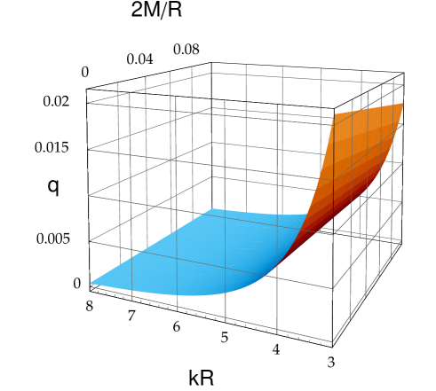
Figure 4: Reflection coefficient $q_{2}=|\gamma_{2}(kR,2M/R)|$ truncated to first order in $2M/R$ as a function of $kR$ and $2M/R$, for the boundary condition $\partial_{t}\Psi_{0}\;\hat{=}\;0$. Showing surface for $3\leq kR\leq 8$.

V.4 Reflection coefficient for the improved boundary condition

Finally, we repeat the above analysis for the boundary condition

$$(\partial_{t}+\partial_{r})(r^{4}\partial_{t}\psi_{0})(t,R)=0,$$ (125)

which is perfectly absorbing for $M=0$ (see Eq. (95)). From Eqs. (120,121) we first obtain

$$4r(\partial_{t}+\partial_{r})(r^{4}\psi_{0\nearrow})(t,r) = \frac{2M}{r}\left[U(r_{*}-t)+rU^{(1)}(r_{*}-t)-15\int\limits_{0}^{\infty}\frac{U(r_{*}-t+2ry)dy}{(1+y)^{7}}\right]+O\left(\frac{2M}{R}\right)^{2}$$

$$4r(\partial_{t}+\partial_{r})(r^{4}\psi_{0\nwarrow})(t,r) = \frac{4}{3}r^{5}V^{(5)}(r_{*}+t)+O\left(\frac{2M}{R}\right).$$

Using the monochromatic ansatz (122), we obtain

$$\Big{|}\gamma_{2,2}\left(kR,\frac{2M}{R}\right)\Big{|}=\frac{2M}{R}\tilde{E}(kR)+O\left(\frac{2M}{R}\right)^{2},$$ (126)

where

$$\tilde{E}(z)=\frac{3}{4z^{5}}\left[\left(1-15C_{7}(z)\right)^{2}+\left(z-15S_{7}(z)\right)^{2}\right]^{1/2}.$$ (127)

For $kR\gg 1$, the reflection coefficient goes as $(2M/R)(kR)^{-4}$. Because of the presence of the small factor $(2M/R)$, there is a significant improvement over the boundary condition $\partial_{t}\Psi_{0}\;\hat{=}\;0$. In Figure 5, we plot the ratio $\tilde{E}(kR)/|\gamma_{2}(kR)|$ as a function of $kR$. This plot, together with the asymptotic expansion $2\tilde{E}(z)/|\gamma_{2}(z)|=1-8z^{-2}+O(z^{-3})$, suggest that for $kR>1.04$, this ratio does not exceed $0.5$. Thus, we conclude that with corrections for backscatter, our improved boundary condition gives a reflection coefficient which is $M/R$ times smaller than the one for the freezing $\Psi_{0}$ condition for $kR>1.04$.

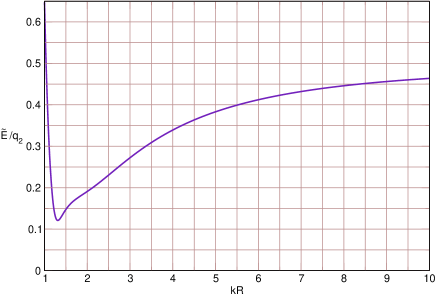
Figure 5: $\tilde{E}(kR)/|\gamma_{2}(kR)|$ versus $kR$.

VI Conclusions

Numerical relativity groups around the world have begun to calculate binary black hole merger waveforms [34, 56, 57, 58, 59, 60, 61, 62, 63, 64, 65, 66], with the goal of providing waveform templates for the detection and interpretation of gravitational wave signals from instruments such as LIGO, VIRGO and LISA. To be useful templates, the calculated waveforms must be as accurate as possible. In particular, if numerical binary black hole simulations are performed on a finite computational grid with an artificial outer boundary, it is critical that this boundary be as seamless an interface as possible between the physical scenario and the computational grid. Towards this end, we have constructed a hierarchy ${\cal B}_{L}$, $L=1,2,3,...$ of boundary conditions which are perfectly absorbing for linearized waves with arbitrary angular momentum number $\ell\leq L$ on a Minkowski background with a spherical outer boundary. For a nonlinear Cauchy formulation of Einstein’s vacuum field equations, these boundary conditions can be formulated as follows. Let $t$ be the time-like coordinate compatible with the foliation $\Sigma_{t}$ by space-like hypersurfaces (ie. such that $\Sigma_{t}=\{t=const\}$), and let $r$ be a radial coordinate which has the property that the two-surfaces $S_{t,r}$ of constant $t$ and $r$ are approximate metric spheres with area $4\pi r^{2}$ for large $r$. We assume that the outer boundary is described, for each $t\geq 0$, by the two-surface $S_{t,R}$. Let $n^{a}$ be the future-directed unit normal to the surfaces $\Sigma_{t}$ and let $s^{a}$ be the normal to the surfaces $S_{t,r}$ tangent to $\Sigma_{t}$. Finally, let $v^{a}$ and $w^{a}$ be two mutually orthogonal unit vector fields which are normal to $n^{a}$ and $s^{a}$, and define the real null vector $l^{a}=(n^{a}+s^{a})/\sqrt{2}$ and the complex null vector $m^{a}=(v^{a}+iw^{a})/\sqrt{2}$. Then, for each $L\geq 1$, the boundary condition ${\cal B}_{L}$ is

$$\frac{\partial}{\partial t}\left.\left[r^{2}l^{a}\nabla_{a}\right]^{L-1}\left(r^{5}\Psi_{0}\right)\right|_{r=R}=0,$$ (128)

where $\nabla_{a}$ denotes the covariant derivative with respect to the four metric and where, in terms of the Weyl tensor $C_{abcd}$, the Newman-Penrose scalar $\Psi_{0}$ is given by $\Psi_{0}=C_{abcd}l^{a}m^{b}l^{c}m^{d}$. For $L=1$, this reduces to the freezing $\Psi_{0}$ boundary condition proposed in [17, 16, 19, 18, 21]. The new boundary conditions (128) are local in time and space, and do not depend on the spherical harmonic decomposition. Although they require higher order derivatives of the fields at the boundary, high-order derivatives can be eliminated by introducing auxiliary variables at the boundary (for example, see Ref. [5]).

Additionally, we have calculated reflection coefficients which quantify the amount of spurious radiation reflected into the computational domain both by our new hierarchy of boundary conditions ${\cal B}_{L}$ together with constraint-preserving boundary conditions (CBPC), and by CPBC currently in use, which freeze the Newman-Penrose scalar $\Psi_{0}$ to its initial value. Including corrections for backscatter, our new boundary conditions, although no longer perfectly absorbing, give a reflection coefficient for odd-parity quadrupolar radiation which is less than the one for the freezing $\Psi_{0}$ condition by a factor of $M/R$ for $kR>1.04$. (We expect a similar result to hold for even-parity quadrupolar radiation.)

An application of our results to simulations of the full nonlinear Einstein equations requires that: (i) the spacetime near the outer boundary of the computational domain be accurately described by the linearized field equations, (ii) the cross sections of the outer boundary surface with the foliation $\Sigma_{t}$ be approximate metric two-spheres of constant area, (iii) the foliation $\Sigma_{t}$ near the outer boundary resemble the $t=const.$ foliation of Minkowksi space, where $t$ is the standard Minkowski time coordinate, and (iv) the magnitude of the normal component of the shift vector at the outer boundary be small compared to one. Criteria (i) and (ii) are fully justified because modern numerical relativity codes can push the outer boundary into the weak field regime by using mesh refinement, and can handle spherical outer boundaries using multi-block finite differencing [39, 40, 41] or pseudo-spectral methods [42, 23]. However, criteria (iii) and (iv) are more restrictive because they place requirements on the coordinate and slicing conditions. For example, using maximal slicing or a slicing which insures that the mean curvature rapidly decays to zero as one approaches the outer boundary might justify criterion (iii), while forcing the normal component (with respect to the outer boundary) of the shift vector to be zero at the outer boundary guarantees (iv). On the other hand, these criteria are not justified if hyperboloidal slices are used [67, 37, 68, 69], where the mean curvature asymptotically approaches a constant, nonzero value. It should not be difficult to generalize our analysis to more general foliations of Minkowski spacetime using the $2+1$ split discussed in Sect. II.2.

The new boundary conditions (128) constructed in this article should be useful for improving the accuracy of binary black hole calculations on finite domains. For example, if the outer boundary is spherical with area $4\pi R^{2}$ and $R>100M$, then the reflection coefficient for CPBC with freezing $\Psi_{0}$ is less than $0.1\%$ for quadrupolar waves with wavelength $100M$ or smaller. Since the energy flux scales as the amplitude of the wave squared, this reflected false radiation causes a relative error in the energy flux calculation for quadrupolar radiation of the order $10^{-6}$ or less. If one uses the improved boundary condition ${\cal B}_{2}$ proposed in this article instead of the freezing $\Psi_{0}$ condition, then the reflection coefficient is $100\times$ smaller; ie. less than $0.001\%$. Correspondingly, the contribution of reflected artefactual radiation to the relative error in the energy flux calculation for odd-parity quadrupolar radiation is below $10^{-10}$. Finally, the improved boundary conditions presented here may be useful for minimizing reflections of “junk” radiation present in the initial data.

We would like to conclude by emphasizing two points. The first point is that the hierarchy of new boundary conditions ${\cal B}_{L}$ proposed in this article (128) are not restricted to the Bianchi equations, but can be applied to any formulation of Einstein’s field equations. It is important that they are used in conjunction with CPBC and suitable boundary conditions which control part of the geometry of the outer boundary surface (in particular, they should insure that the outer boundary remains spherical and that its area does not change too much in time). While these last two types of boundary conditions depend explicitly on the formulation, condition (128) does not. After all these boundary conditions have been specified, one still needs to show that the resulting IBVP is well posed. This issue is one which we will address elsewhere. The estimates of the reflection coefficients for spurious gravitational radiation given in this article are valid for any representation of the Einstein equations which implements the freezing $\Psi_{0}$ boundary condition together with CPBC. In particular, they are directly applicable to the formulations in [12, 17, 16, 19, 18, 21].

The second point is that our improved boundary conditions may not be transparent enough to model accurately all physically interesting scenarios on an unbounded domain. For example, it is likely that even with our new boundary conditions, one will find an incorrect tail decay when measuring the decay of solutions at a fixed location near the outer boundary. The failure of the simple Sommerfeld condition to correctly simulate tail decays for a spherically symmetric scalar field about a Schwarzschild black hole was demonstrated numerically in [70]. In fact, the work in [71] proves analytically that the boundary conditions in [70] lead to decay which is faster than any power of $1/t$ (whereas the expected rate of decay is $1/t^{3}$ [72]). For future work, we plan to explore ways to improve our new boundary conditions to reproduce correctly the tail decay. One possibility is to use the work in [8, 9, 10] to construct boundary conditions which are perfectly absorbing when backscatter is considered.

Appendix A Stability of the absorbing boundary conditions

In this appendix, we consider the initial-boundary value problem

$$\left[\partial_{t}^{2}-\partial_{r}^{2}+\frac{\ell(\ell+1)}{r^{2}}\right]\phi(t,r)=0,\qquad t>0,\quad R_{0}<r<R,$$ (129)

$$\phi(0,r)=f(r),\qquad\partial_{t}\phi(0,r)=g(r),\qquad R_{0}<r<R,$$ (130)

$$(b_{+})^{L+1}\partial_{t}\phi(t,R_{0})=0,\qquad(b_{-})^{L+1}\partial_{t}\phi(t,R)=0,\qquad t>0,$$ (131)

where $\ell$, $L$ are natural numbers, $0<R_{0}<R$ are the inner and outer radii of a spherical shell, $f$ and $g$ are smooth initial data, and $b_{\pm}=r^{2}(\partial_{t}\mp\partial_{r})$. The reason for introducing the inner boundary at $r=R_{0}$ is to excise the coordinate singularity at $r=0$. This is not a restriction for the purpose of this article, since we are interested only in the region near the outer boundary, and since we consider the linearized equations for modeling a physical scenario away from the strong field region.

In order to show that the problem (129,130,131) is stable in the sense that the solution depends continuously on the data, we introduce the following notation:

$$\Phi_{j}^{(\pm)}=(b_{\pm})^{j}\phi,\qquad j=0,1,2,3,...$$

Notice that $\Phi_{0}^{(+)}=\Phi_{0}^{(-)}=\phi$. By applying the operators $b_{+}$ and $b_{-}$ to both sides of Eq. (129), one finds the formula

$$b_{\mp}(\Phi_{j}^{(\pm)})=\pm 2jr\Phi_{j}^{(\pm)}-(\ell-j+1)(\ell+j)r^{2}\Phi_{j-1}^{(\pm)}$$

for $j=1,2,3,...$. Using this and $b_{\pm}(\Phi_{j}^{(\pm)})=\Phi_{j+1}^{(\pm)}$, we find that

$$2r^{2}\partial_{t}(\Phi_{j}^{(\pm)})=(b_{+}+b_{-})\Phi_{j}^{(\pm)}=\pm 2jr\Phi_{j}^{(\pm)}-(\ell-j+1)(\ell+j)r^{2}\Phi_{j-1}^{(\pm)}+\Phi_{j+1}^{(\pm)}$$

for all $j=1,2,3,...$. Therefore, the evolution equations (129) and the boundary conditions (131) yield the evolution system

$$\partial_{t}\Phi_{0} = \frac{1}{2r^{2}}\left(\Phi_{1}^{(+)}+\Phi_{1}^{(-)}\right),$$ (132)

$$\partial_{t}\Phi_{j}^{(+)} = \frac{1}{2r^{2}}\Phi_{j+1}^{(+)}+\frac{j}{r}\Phi_{j}^{(+)}-\frac{(\ell-j+1)(\ell+j)}{2}\Phi_{j-1}^{(+)},\qquad j=1,2,...L,$$ (133)

$$\partial_{t}\Phi_{j}^{(-)} = \frac{1}{2r^{2}}\Phi_{j+1}^{(-)}-\frac{j}{r}\Phi_{j}^{(-)}-\frac{(\ell-j+1)(\ell+j)}{2}\Phi_{j-1}^{(-)},\qquad j=1,2,...L,$$ (134)

$$(\partial_{t}+\partial_{r})\Phi_{L+1}^{(+)} = \frac{2(L+1)}{r}\Phi_{L+1}^{(+)}-(\ell-L)(\ell+L+1)\Phi_{L}^{(+)},$$ (135)

$$(\partial_{t}-\partial_{r})\Phi_{L+1}^{(-)} = -\frac{2(L+1)}{r}\Phi_{L+1}^{(-)}-(\ell-L)(\ell+L+1)\Phi_{L}^{(-)},$$ (136)

with boundary conditions

$$\partial_{t}\Phi_{L+1}^{(+)}(t,R_{0})=0,\qquad\partial_{t}\Phi_{L+1}^{(-)}(t,R)=0,\qquad t>0.$$ (137)

The system (132,133,134,135,136) constitutes a symmetric hyperbolic system with maximally dissipative boundary conditions (137). It is well-known (see, for example, Ref. [73]) that such systems are well posed and admit energy estimates. For example, it follows that a smooth enough solution satisfies the estimate

$$E(t)\leq e^{bt}E(0)$$ (138)

with the energy norm

$$E(t)=\frac{1}{2}\int\limits_{R_{0}}^{R}\left(r^{2(L+1)}\Phi_{0}^{2}(t,r)+\sum\limits_{j=1}^{L+1}r^{2(L+1-j)}\left[(\Phi_{j}^{(+)}(t,r))^{2}+(\Phi_{j}^{(-)}(t,r))^{2}\right]\right)dr,$$

where $b$ is a constant that does not depend on the solution. In particular, the inequality (138) implies that the solutions depend uniquely and continuously on the initial data. The existence of solutions (including for evolution equations with more general potentials than the one in Eq. (129)) can be proved using methods from semigroup theory; see for example chapter 6.3 in [74] for a well posedness proof for a similar problem. A different well posedness proof based on the verification of the Kreiss condition is given in [3].

Since for $\ell\leq L$, the exact outgoing solutions $\phi_{\nearrow,\ell}(t,r)$ constructed in Sect. III.2 satisfy the boundary conditions (131), provided the function $U_{\ell}$ is compactly supported in $(R_{0},R)$, it follows that the boundary conditions (131) are perfectly absorbing for all $\ell\leq L$.

References

- [1] D. Givoli. Non-reflecting boundary conditions. J. Comp. Phys., 94:1–29, 1991.
- [2] B. Engquist and A. Majda. Absorbing boundary conditions for the numerical simulation of waves. Math. Comp., 31:629–651, 1977.
- [3] A. Bayliss and E. Turkel. Radiation boundary conditions for wave-like equations. Comm. Pure and Appl. Math., 33:707–725, 1980.
- [4] R. L. Higdon. Absorbing boundary conditions for difference approximations to the multi-dimensional wave equations. Math. Comp., 47:437–459, 1986.
- [5] D. Givoli. High-order nonreflecting boundary conditions without high-order derivatives. J. Comp. Phys., 170:849–870, 2001.
- [6] D. Givoli and B. Neta. High-order non-reflecting boundary scheme for time-dependent waves. J. Comp. Phys., 186:24–46, 2003.
- [7] B. Alpert, L. Greengard, and T. Hagstrom. Rapid evaluation of nonreflecting boundary kernels for time-domain wave propagation. SIAM J. Numer. Anal., 37:1138–1164, 2000.
- [8] S. R. Lau. Rapid evaluation of radiation boundary kernels for time-domain wave propagation on blackholes: theory and numerical methods. J. Comput. Phys., 199:376–422, 2004.
- [9] S. R. Lau. Rapid evaluation of radiation boundary kernels for time-domain wave propagation on black holes: implementation and numerical tests. Class. Quantum Grav., 21:4147–4192, 2004.
- [10] S. R. Lau. Analytic structure of radiation boundary kernels for blackhole perturbations. J. Math. Phys., 46:102503(1)–102503(21), 2005.
- [11] J.M. Bardeen and L.T. Buchman. Numerical tests of evolution systems, gauge conditions, and boundary conditions for 1d colliding gravitational plane waves. Phys. Rev. D, 65:064037(1)–064037(23), 2002.
- [12] H. Friedrich and G. Nagy. The initial boundary value problem for Einstein’s vacuum field equations. Comm. Math. Phys., 201:619–655, 1999.
- [13] P. Secchi. Well-posedness of characteristic symmetric hyperbolic systems. Arch. Rat. Mech. Anal., 134:155–197, 1996.
- [14] B. Szilagyi and J. Winicour. Well-posed initial-boundary evolution in general relativity. Phys. Rev. D, 68:041501(1)–041501(5), 2003.
- [15] G. Calabrese, J. Pullin, O. Reula, O. Sarbach, and M. Tiglio. Well posed constraint-preserving boundary conditions for the linearized Einstein equations. Comm. Math. Phys., 240:377–395, 2003.
- [16] O. Sarbach and M. Tiglio. Boundary conditions for Einstein’s field equations: Mathematical and numerical analysis. Journal of Hyperbolic Differential Equations, 2:839–883, 2005.
- [17] L.E. Kidder, L. Lindblom, M.A. Scheel, L. Buchman, and H.P. Pfeiffer. Boundary conditions for the Einstein evolution system. Phys. Rev. D, 71:064020(1)–064020(22), 2005.
- [18] L. Lindblom, M.A. Scheel, L.E. Kidder, R. Owen, and O. Rinne. A new generalized harmonic evolution system. Class. Quantum Grav., 23:S447–S462, 2006.
- [19] G. Nagy and O. Sarbach. A minimization problem for the lapse and the initial-boundary value problem for Einstein’s field equations. Class. Quantum Grav., 23:S477–S504, 2006.
- [20] H. O. Kreiss and J. Winicour. Problems which are well-posed in a generalized sense with applications to the Einstein equations. Class. Quantum Grav., 23:S405–S420, 2006.
- [21] O. Rinne. Stable radiation-controlling boundary conditions for the generalized harmonic Einstein equations, 2006. gr-qc/0606053.
- [22] J. Novak and S. Bonazzola. Absorbing boundary conditions for simulation of gravitational waves with spectral methods in spherical coordinates. J. Comp. Phys., 197:186–196, 2004.
- [23] S. Bonazzola, E. Gourgoulhon, P. Grandcl\a’ement, and J. Novak. Constrained scheme for the Einstein equations based on the Dirac gauge and spherical coordinates. Phys. Rev. D, 70:104007(1)–104007(24), 2004.
- [24] A. M. Abrahams and C. R. Evans. Reading off the gravitational radiation waveforms in numerical relativity calculations: Matching to linearized gravity. Phys. Rev. D, 37:318–332, 1988.
- [25] A. M. Abrahams and C. R. Evans. Gauge-invariant treatment of gravitational radiation near the source: Analysis and numerical simulations. Phys. Rev. D, 42:2585–2594, 1990.
- [26] A. M. Abrahams et al.[Binary Black Hole Grand Challenge Alliance Collaboration]. Cauchy-perturbative matching and outer boundary conditions by perturbative matching. Phys. Rev. Lett., 80:1812–1815, 1998.
- [27] M. E. Rupright, A. M. Abrahams, and L. Rezzolla. Cauchy-perturbative matching and outer boundary conditions: I: Methods and tests. Phys. Rev. D, 58:044005(1)–044005(9), 1998.
- [28] L. Rezzolla, A. M. Abrahams, R. A. Matzner, M. E. Rupright, and S. L. Shapiro. Cauchy-perturbative matching and outer boundary conditions: Computational studies. Phys. Rev. D, 59:064001(1)–064001(17), 1999.
- [29] B. Zink, E. Pazos, P. Diener, and M. Tiglio. Cauchy-perturbative matching revisited: Tests in spherical symmetry. Phys. Rev. D, 73:084011(1)–084011(14), 2006.
- [30] J. Winicour. Characteristic evolution and matching. Living Rev. Relativity, 3, 2001.
- [31] G. Calabrese. Exact boundary conditions in numerical relativity using multiple grids: Scalar field tests, 2006. gr-qc/0604034.
- [32] L. Lehner. Matching characteristic codes: Exploiting two directions. Int. J. Mod. Phys. D, 9:469–474, 2000.
- [33] M. Choptuik, L. Lehner, I. Olabarrieta, R. Petryk, F. Pretorius, and H. Villegas. Towards the final fate of an unstable black string. Phys. Rev. D, 68:044001(1)–044001(11), 2003.
- [34] F. Pretorius. Evolution of binary black-hole spacetimes. Phys. Rev. Lett., 95:121101(1)–121101(4), 2005.
- [35] H. Friedrich. On the regular and asymptotic characteristic initial value problem for Einstein’s vacuum field equations. Proc. Roy. Soc. Lond., A375:169–184, 1981.
- [36] J. Frauendiener. Numerical treatment of the hyperboloidal initial value problem for the vacuum Einstein equations. 2. the evolution equations. Phys. Rev. D, 58:064003(1)–064003(18), 1998.
- [37] C S. Husa, Schneemann, T. Vogel, and A. Zenginoglu. Hyperboloidal data and evolution. To appear in the proceedings of 28th Spanish Relativity Meeting (ERE05): A Century of Relativity Physics, Oviedo, Asturias, Spain, 6-10 Sep 2005, 2005. gr-qc/0512033.
- [38] J. M. Stewart and M. Walker. Perturbations of space-times in general relativity. Proc. R. Soc. Lond. A, 341:49–74, 1974.
- [39] J. Thornburg. Black hole excision with multiple grid patches. Class. Quantum Grav., 21:3665–3692, 2004.
- [40] L. Lehner, O. Reula, and M. Tiglio. Multi-block simulations in general relativity: High order discretizations, numerical stability, and applications. Class. Quantum Grav., 22:5283–5322, 2005.
- [41] E. Schnetter, P. Diener, E. N. Dorband, and M. Tiglio. A multi-block infrastructure for three-dimensional time-dependent numerical relativity. Class. Quantum Grav., 23:S553–S578, 2006.
- [42] L. E. Kidder, M. A. Scheel, and S. A. Teukolsky. Extending the lifetime of 3-D black hole computations with a new hyperbolic system of evolution equations. Phys. Rev. D, 64:064017(1)–064017(13), 2001.
- [43] J. M. Bardeen and W. H. Press. Radiation fields in the Schwarzschild background. J. Math. Phys., 14:7–19, 1973.
- [44] S.A. Teukolsky. Rotating black holes: Separable wave equations for gravitational and electromagnetic perturbations. Phys. Rev. Lett., 29:1114–1118, 1972.
- [45] F. B. Estabrook and H. D. Wahlquist. Dyadic analysis of space-time congruences. J. Math. Phys., 5:1629–1644, 1964.
- [46] H. Friedrich. Hyperbolic reductions for Einstein’s equations. Class. Quantum Grav., 13:1451–1469, 1996.
- [47] F. B. Estabrook, R. S. Robinson, and H. D. Wahlquist. Hyperbolic equations for vacuum gravity using special orthonormal frames. Class. Quantum Grav., 14:1237–1247, 1997.
- [48] H. Friedrich and A. D. Rendall. The cauchy problem for the Einstein equations. Lect. Notes Phys., 540:127–224, 2000.
- [49] E. T. Newman and R. Penrose. An approach to gravitational radiation by a method of spin coefficients. J. Math. Phys., 3:566–578, 1962. erratum 4 998(E) (1963).
- [50] W. L. Burke. Gravitational radiation damping of slowly moving systems calculated using matched asymptotic expansions. J. Math. Phys., 12:401–418, 1971.
- [51] S.A. Teukolsky. Linearized quadrupole waves in general relativity and the motion of test particles. Phys. Rev. D, 26:745–750, 1982.
- [52] R. Penrose. Zero rest-mass fields including gravitation: asymptotic behaviour. Proc. Roy. Soc. Lond. A, 284:159–203, 1965.
- [53] N.T. Bishop, R. Gomez, L. Lehner, B. Szilagyi, J. Winicour, and R. A. Isaacson. Cauchy characteristic matching. In Black holes, gravitational radiation and the universe, pages 383–408. Kluwer, 1998. gr-qc/9801070.
- [54] R. H. Price. Nonspherical perturbations of relativistic gravitational collapse. II. Integer-spin, zero-rest-mass fields. Phys. Rev. D, 5:2439–2454, 1972.
- [55] T. Regge and J. Wheeler. Stability of a Schwarzschild singularity. Phys. Rev., 108:1063–1069, 1957.
- [56] F. Pretorius. Simulation of binary black hole spacetimes with a harmonic evolution scheme, 2006. gr-qc/0602115.
- [57] M. Campanelli, C. O. Lousto, and Y. Zlochower. Last orbit of binary black holes. Phys. Rev. D, 73:061501(1)–061501(5), 2006.
- [58] J. G. Baker, J. Centrella, D.-I. Choi, M. Koppitz, and J. van Meter. Binary black hole merger dynamics and waveforms. Phys. Rev. D, 73:104002(1)–104002(11), 2006.
- [59] M. Campanelli, C. O. Lousto, P. Marronetti, and Y. Zlochower. Accurate evolutions of orbiting black-hole binaries without excision. Phys. Rev. Lett., 96:111101(1)–111101(4), 2006.
- [60] J. G. Baker, J. Centrella, D.-I. Choi, M. Koppitz, and J. van Meter. Gravitational-wave extraction from an inspiraling configuration of merging black holes. Phys. Rev. Lett., 96:111102(1)–111102(4), 2006.
- [61] P. Diener, F. Herrmann, D. Pollney, E. Schnetter, E. Seidel, R. Takahashi, J. Thornburg, and J. Ventrella. Accurate evolution of orbiting binary black holes. Phys. Rev. Lett., 96:121101(1)–121101(4), 2006.
- [62] F. Herrmann, D. Shoemaker, and P. Laguna. Unequal-mass binary black hole inspirals, 2006. gr-qc/0601026.
- [63] J. G. Baker, J. Centrella, D.-I. Choi, M. Koppitz, J. van Meter, and M. C. Miller. Getting a kick out of numerical relativity, 2006. astro-ph/0603204.
- [64] M. Campanelli, C. O. Lousto, and Y. Zlochower. Gravitational radiation from spinning-black-hole binaries: The orbital hang up, 2006. gr-qc/0604012.
- [65] U. Sperhake. Binary black-hole evolutions of excision and puncture data, 2006. gr-qc/0606079.
- [66] M. A. Scheel, H. P. Pfeiffer, L. Lindblom, L. E. Kidder, O. Rinne, and S. A. Teukolsky. Solving Einstein’s equations with dual coordinate frames, 2006. gr-qc/0607056.
- [67] J. Frauendiener and T. Vogel. Algebraic stability analysis of constraint propagation. Class.Quantum Grav., 22:1769–1793, 2005.
- [68] G. Calabrese, C. Gundlach, and D. Hilditch. Asymptotically null slices in numerical relativity: mathematical analysis and spherical wave equation tests. Class.Quantum Grav., 23:4829–4845, 2006.
- [69] L. T. Buchman and J. M. Bardeen. Schwarzschild tests of the Wahlquist-Estabrook-Buchman-Bardeen tetrad formulation for numerical relativity. Phys. Rev. D, 72:124014(1)–124014(14), 2005.
- [70] E. W. Allen, E. Buckmiller, L. M. Burko, and R. H. Price. Radiation tails and boundary conditions for black hole evolutions. Phys. Rev. D, 70:044038(1)–044038(5), 2004.
- [71] M. Dafermos and I. Rodnianski. A note on boundary value problems for black hole evolutions, 2004. gr-qc/0403034.
- [72] R. H. Price. Nonspherical perturbations of relativistic gravitational collapse. I. Scalar and gravitational perturbations. Phys. Rev. D, 5:2419–2438, 1972.
- [73] H. O. Kreiss and J. Lorenz. Initial-Boundary Value Problems and the Navier-Stokes Equations. Academic Press, 1989.
- [74] H. Beyer. Beyond partial differential equations: A course on linear and quasi-linear abstract evolution equations. http://xxx.lanl.gov/abs/gr-qc/0510097.
- [75] H. L. Royden. Real Analysis. Macmillan Publishing Company, New York, 1989.