Generalizing Starobinskiĭ’s Formalism to Yukawa Theory & to Scalar QED

Abstract

During inflation quantum effects from massless, minimally coupled scalars and gravitons can be strengthened so much that perturbation theory breaks down. To follow the subsequent evolution one must employ a nonperturbative resummation. Starobinskiĭ has developed such a technique for simple scalar theories. I discuss recent progress in applying this technique to more complicated models.

1 Introduction

On cosmological scales the universe is well described by a homogeneous, isotropic and spatially flat geometry,

$$ds^{2}=-dt^{2}+a^{2}(t)d\vec{x}\cdot d\vec{x}\;.$$ (1)

Derivatives of the scale factor $a(t)$ give the Hubble parameter $H(t)$ and the deceleration parameter $q(t)$,

$$H(t)\equiv\frac{\dot{a}}{a}\qquad,\qquad q(t)\equiv-\frac{a\ddot{a}}{\dot{a}^{2}}=-1-\frac{\dot{H}}{H^{2}}\;.$$ (2)

Inflation is defined as positive expansion ($H(t)>0$) with negative deceleration ($q(t)<0$).

The homogeneity of spacetime expansion evident in (1) does not change the fact that particles have constant wave vectors $\vec{k}$, but it does alter what these mean physically. In particular the energy of a particle with mass $m$ and wave number $k=\|\vec{k}\|$ becomes time dependent,

$$E(t,k)=\sqrt{m^{2}+\Bigl{(}k/a(t)\Bigr{)}^{2}}\;.$$ (3)

This results in an interesting change in the energy-time uncertainty principle which restricts how long a virtual pair of such particles with $\pm\vec{k}$ can exist. If the pair was created at time $t$, it can last a time $\Delta t$ given by the integral,

$$\int_{t}^{t+\Delta t}\!\!\!\!\!dt^{\prime}E(t^{\prime},k)\sim 1\;.$$ (4)

Just as in flat space, particles with the smallest masses persist longest. For the fully massless case the wave number factors out, leaving an integral which can be recognized as the radius of the forward light-cone from time $t$ to time $t+{\Delta t}$ [1],

$$\int_{t}^{t+\Delta t}\!\!\!\!\!dt^{\prime}E(t^{\prime},k)\Bigl{|}_{m=0}=k\int_{t}^{t+\Delta t}\!\!\frac{dt^{\prime}}{a(t^{\prime})}\simeq\frac{k}{q(t^{\prime})H(t^{\prime})a(t^{\prime})}\Bigl{|}^{t+{\Delta t}}_{t}\;.$$ (5)

For positive deceleration the upper limit dominates and the integral grows without bound as ${\Delta t}$ increases. In this case the persistence time ${\Delta t}$ is finite, although longer than in flat space. However, for negative deceleration (inflation) it is the lower limit that dominates, and the integral approaches a finite value as ${\Delta t}$ goes to infinity. For example, the result for de Sitter ($a(t)=e^{Ht}$ with $H$ constant) is,

$$k\int_{t}^{t+\Delta t}\!\!\frac{dt^{\prime}}{a(t^{\prime})}\Bigl{|}_{\rm de\ Sitter}=\frac{k}{Ha(t)}\Bigl{[}1-e^{-H\Delta t}\Bigr{]}\;.$$ (6)

Therefore, any massless virtual particle which happens to emerge from the vacuum with $k\mathrel{\raise 1.29167pt\hbox{$<$\kern-11.00008pt\lower 4.30554pt\hbox{ $\sim$}}}H(t)a(t)$ can persist forever!

Most massless particles possess conformal invariance. The change of variables $d\eta\equiv dt/a(t)$ defines a conformal time in terms of which the invariant element (1) is just a conformal factor times that of flat space,

$$ds^{2}=-dt^{2}+a^{2}(t)d\vec{x}\cdot d\vec{x}=a^{2}\Bigl{(}-d\eta^{2}+d\vec{x}\cdot d\vec{x}\Bigr{)}\;.$$ (7)

In the $(\eta,\vec{x})$ coordinates, conformally invariant theories are locally identical to their flat space cousins. The rate at which virtual particles emerge from the vacuum per unit conformal time must be the same constant — call it $\Gamma$ — as in flat space. Hence the rate of emergence per unit physical time is,

$$\frac{dN}{dt}=\frac{dN}{d\eta}\frac{d\eta}{dt}=\frac{\Gamma}{a(t)}\;.$$ (8)

It follows that, although any sufficiently long wavelength, massless and conformally invariant particle which emerges from the vacuum can persist forever during inflation, very few will emerge.

Two kinds of massless particles do not possess conformal invariance: minimally coupled scalars and gravitons. To see that the production of these particles is not suppressed during inflation note that each polarization and wave number behaves like a harmonic oscillator,

$$L=\frac{1}{2}m\dot{q}^{2}-\frac{1}{2}m\omega^{2}q^{2}\;,$$ (9)

with time dependent mass $m(t)=a^{3}(t)$ and frequency $\omega(t)=\frac{k}{a(t)}$. The Heisenberg equation of motion can be solved in terms of mode functions $u(t,k)$ and canonically normalized raising and lowering operators $\alpha^{\dagger}$ and $\alpha$,

$$\ddot{q}+3H\dot{q}+\frac{k^{2}}{a^{2}}q=0\quad\Longrightarrow\quad q(t)=u(t,k)\alpha+u^{*}(t,k)\alpha^{\dagger}\quad{\rm with}\quad[\alpha,\alpha^{\dagger}]=1\;,$$ (10)

The mode functions $u(t,k)$ are quite complicated for a general scale factor $a(t)$ [2] but they take a simple form for de Sitter,

$$u(t,k)=\frac{H}{\sqrt{2k^{3}}}\Bigl{[}1-\frac{ik}{Ha(t)}\Bigr{]}\exp\Bigl{[}\frac{ik}{Ha(t)}\Bigr{]}\;.$$ (11)

The (co-moving) energy operator for this system is,

$$E(t)=\frac{1}{2}m(t)\dot{q}^{2}(t)+\frac{1}{2}m(t)\omega^{2}(t)q^{2}(t)\;.$$ (12)

Owing to the time dependent mass and frequency, there are no stationary states for this system. At any given time the minimum eigenstate of $E(t)$ has energy $\frac{1}{2}\omega(t)$, but which state this is changes for each value of time. The state $|\Omega\rangle$ which is annihilated by $\alpha$ has minimum energy in the distant past. The expectation value of the energy operator in this state is,

$$\Bigl{\langle}\Omega\Bigl{|}E(t)\Bigr{|}\Omega\Bigr{\rangle}=\frac{1}{2}a^{3}(t)|\dot{u}(t,k)|^{2}+\frac{1}{2}a(t)k^{2}|u(t,k)|^{2}\Bigl{|}_{\rm de\ Sitter}=\frac{k}{2a}+\frac{H^{2}a}{4k}\;.$$ (13)

If one thinks of each particle having energy $k/a(t)$, it follows that the number of particles with any polarization and wave number $k$ grows as the square of the inflationary scale factor,

$$N(t,k)=\Bigl{(}\frac{Ha(t)}{2k}\Bigr{)}^{2}\;!$$ (14)

Quantum field theoretic effects are driven by essentially classical physics operating in response to the source of virtual particles implied by quantization. On the basis of (14) one might expect inflation to dramatically enhance quantum effects from MMC scalars and gravitons, and explicit studies over a quarter century have confirmed this. The oldest results are of course the cosmological perturbations induced by scalar inflatons [3] and by gravitons [4]. More recently it was shown that the one loop vacuum polarization induced by a charged MMC scalar in de Sitter background causes super-horizon photons to behave like massive particles in some ways [5, 6, 7]. Another recent result is that the one loop fermion self-energy induced by a MMC Yukawa scalar in de Sitter background reflects the generation of a nonzero fermion mass [8, 9]. In the next three sections it will be explicitly shown how these one loop results generalize to all orders.

2 Infrared Logarithms

The expectation values of familiar operators typically show enhanced quantum effects in the form of infrared logarithms. A simple example is provided by the stress tensor of a massless, minimally coupled scalar with a quartic self-interaction,

$$\mathcal{L}=-\frac{1}{2}\partial_{\mu}\varphi\partial_{\nu}\varphi g^{\mu\nu}\sqrt{-g}-\frac{\lambda}{4!}\varphi^{4}\sqrt{-g}+{\rm counterterms}\;.$$ (15)

When the expectation value of the stress tensor of this theory is computed in de Sitter background ($a(t)=e^{Ht}$) and renormalized so as to make quantum effects vanish at $t=0$, the results for the quantum-induced energy density and pressure are [10, 11],

$$\rho(t) = \frac{\lambda H^{4}}{(2\pi)^{4}}\Bigl{\{}\frac{1}{8}\ln^{2}(a)\Bigr{\}}+O(\lambda^{2})\;,$$ (16)

$$p(t) = \frac{\lambda H^{4}}{(2\pi)^{4}}\Bigl{\{}-\frac{1}{8}\ln^{2}(a)-\frac{1}{12}\ln(a)\Bigr{\}}+O(\lambda^{2})\;.$$ (17)

Infrared logarithms are the factors of $\ln(a)=Ht$. They arise from the fact that inflationary particle production drives the free scalar field strength away from zero [12, 13, 14],

$$\Bigl{\langle}\Omega\Bigl{|}\varphi^{2}(x)\Bigr{|}\Omega\Bigr{\rangle}_{0}=\frac{H^{2}}{4\pi^{2}}\ln(a)+{\rm Divergent\ Constant}\;.$$ (18)

This increases the vacuum energy contributed by the quartic potential, and the result is evident in (16-17).

Infrared logarithms arise in the one particle irreducible (1PI) functions of this theory [15]. They occur as well in massless, minimally coupled scalar quantum electrodynamics (SQED) [5, 6, 7] and in massless Yukawa theory [8, 9]. The 1PI functions of pure gravity on de Sitter background show infrared logarithms [16, 17]. It seems inevitable that infrared logarithms contaminate loop corrections to the power spectrum of cosmological perturbations [18, 19] and similar fixed-momentum correlators [20]. And infrared logarithms have been discovered in the 1PI functions and quantum-corrected mode functions of Einsetin + Dirac [21, 22].

Infrared logarithms are fascinating because they introduce a secular element into the usual, static expansion in the loop counting parameter. No matter how small the coupling constant $\lambda$ is in (16-17), the continued growth of the inflationary scale factor must eventually overwhelm it. When this happens, perturbation theory breaks down. For example, the general form of the induced energy density (16) is,

$$\rho(t)=H^{4}\sum_{\ell=2}^{\infty}\lambda^{\ell-1}\Bigl{\{}C^{\ell}_{0}\ln^{2\ell-2}(a)+C^{\ell}_{1}\ln^{2\ell-3}(a)+\ldots+C^{\ell}_{2\ell-4}\ln^{2}(a)\Bigr{\}}\;.$$ (19)

The $C^{\ell}_{0}[\lambda\ln^{2}(a)]^{\ell-1}$ terms are the leading logarithms at $\ell$ loop order; the remaining terms are subdominant logarithms. Assuming that the numerical coefficients $C^{\ell}_{k}$ are of order one, we see that the leading infrared logarithms all become order one at $\ln(a)\sim 1/\sqrt{\lambda}$. At this time the highest subdominant logarithm terms are still perturbatively small ($\sim\sqrt{\lambda}$), so it seems reasonable to attempt to follow the nonperturbative evolution by resuming the series of leading infrared logarithms,

$$\rho_{\rm lead}=H^{4}\sum_{\ell=0}^{\infty}C^{\ell}_{0}\Bigl{(}\lambda\ln^{2}(a)\Bigr{)}^{\ell-1}\;.$$ (20)

This is known as the leading logarithm approximation.

3 Starobinskiĭ’s Formalism for Simple Scalar Models

Starobinskiĭ has long maintained that his stochastic field equations reproduce the leading logarithm approximation [23]. With Yokoyama [24] he exploited this conjecture to explicitly solve for the nonperturbative, late time limit of any model of the form ,

$$\mathcal{L}=-\frac{1}{2}\partial_{\mu}\varphi\partial_{\nu}\varphi g^{\mu\nu}\sqrt{-g}-V(\varphi)\sqrt{-g}\;,$$ (21)

assuming only that the potential $V(\varphi)$ is bounded below. When the potential is unbounded below the conjecture still gives the leading infrared logarithms at each order, however, the theory fails to approach a static limit.

An all orders derivation has recently been given of Starobinskiĭ’s formalism [25, 26]. The first step is to rewrite the operator field equations,

$$\ddot{\varphi}+3H\dot{\varphi}-\frac{\nabla^{2}}{a^{2}}\varphi+V^{\prime}(\varphi)=0\;,$$ (22)

in Yang-Feldman form [27],

$$\varphi(t,\vec{x})=\varphi_{0}(t,\vec{x})-\int_{0}^{t}dt^{\prime}a^{\prime 3}\int d^{3}x^{\prime}G(x;x^{\prime})V^{\prime}\Bigl{(}\varphi(x^{\prime})\Bigr{)}\;.$$ (23)

The free field expansion and retarded Green’s function are,

$$\varphi_{0}(t,\vec{x}) \equiv \int\frac{d^{3}k}{(2\pi)^{3}}\Bigl{\{}u(t,k)e^{i\vec{k}\cdot\vec{x}}\alpha(\vec{k})+u^{*}(t,k)e^{-i\vec{k}\cdot\vec{x}}\alpha^{\dagger}(\vec{k})\Bigr{\}}\;,$$ (24)

$$G(x;x^{\prime}) = i\theta(\Delta t)\int\frac{d^{3}k}{(2\pi)^{3}}e^{i\vec{k}\cdot\Delta\vec{x}}\Bigl{\{}u(t,k)u^{*}(t^{\prime},k)-u^{*}(t,k)u(t^{\prime},k)\Bigr{\}}\;.$$ (25)

The mode function $u(t,k)$ was given in expression (11). The canonically normalized creation and annihilation operators are $\alpha^{\dagger}(\vec{k})$ and $\alpha(\vec{k})$. Iterating the Yang-Feldman equation gives the usual perturbative expansion of the interaction picture field, expressed in terms of a field which is free at $t=0$.

Now consider taking the expectation value of some operator constructed from $\varphi$, and hence from the free field $\varphi_{0}$. To reach leading logarithm order requires that every free field contributes to an infrared logarithm. The full result from the pairing of two free fields is,

$$\Bigl{\langle}\Omega_{0}\Bigl{|}\varphi_{0}(t,\vec{x})\varphi_{0}(t^{\prime},\vec{x}^{\prime})\Bigr{|}\Omega_{0}\Bigr{\rangle}=\frac{1}{2\pi^{2}}\int dkk^{2}\,u(t,k)u^{*}(t^{\prime},k)\frac{\sin(k\Delta x)}{k\Delta x}\;.$$

At high $k$ the mode functions and the $\sin(k\Delta x)$ oscillate, which makes the integral converge. As the name suggests, it is the low $k$ end of the integration which is responsible for infrared logarithms. In this regime $\sin(k\Delta x)/k\Delta x\simeq 1$ and only the first term in the long wavelength expansion of the mode functions matters,

$$u(t,k)=\frac{H}{\sqrt{2k^{3}}}\Bigl{\{}1+\frac{1}{2}\Bigl{(}\frac{k}{Ha}\Bigr{)}^{2}+\frac{i}{3}\Bigl{(}\frac{k}{Ha}\Bigr{)}^{3}+\ldots\Bigr{\}}\;.$$ (26)

This observation has two important consequences:

• The leading logarithm result will not be changed if the free field mode sum is cut off at $k=Ha(t)$; and

• The leading logarithm result will not be changed if the mode function is replaced by its infrared limit.

Together, these simplifications convert the free quantum field to a commuting combination of creation and annihilation operators,

$$\varphi_{0}(t,\vec{x})\longrightarrow\Phi_{0}(t,\vec{x})\equiv\int\frac{d^{3}k}{(2\pi)^{3}}\theta(Ha-k)\frac{H}{\sqrt{2k^{3}}}\Bigl{\{}e^{i\vec{k}\cdot\vec{x}}\alpha(\vec{k})+e^{-i\vec{k}\cdot\vec{x}}\alpha^{\dagger}(\vec{k})\Bigr{\}}\;,$$ (27)

Because the Green’s function involves a commutator of mode functions, its infrared truncation requires third order terms from (26),

$$G(x;x^{\prime}) \longrightarrow i\theta(t-t^{\prime})\int\frac{d^{3}k}{(2\pi)^{3}}e^{i\vec{k}\cdot\Delta\vec{x}}\frac{H^{2}}{k^{3}}\Bigl{\{}\frac{i}{3}\Bigl{(}\frac{k}{Ha}\Bigr{)}^{3}-\frac{i}{3}\Bigl{(}\frac{k}{Ha^{\prime}}\Bigr{)}^{3}\Bigr{\}}\;,$$ (28)

$$= \frac{\theta(t-t^{\prime})}{3H}\Bigl{[}\frac{1}{a^{\prime 3}}-\frac{1}{a^{3}}\Bigr{]}\delta^{3}(\vec{x}-\vec{x}^{\prime})\;.$$ (29)

The infrared truncated Yang-Feldman equation is accordingly,

$$\Phi(t,\vec{x})=\Phi_{0}(t,\vec{x})-\frac{1}{3H}\int_{0}^{t}dt^{\prime}\Bigl{[}1-\Bigl{(}\frac{a^{\prime}}{a}\Bigr{)}^{3}\Bigr{]}V^{\prime}\Bigl{(}\Phi(t^{\prime},\vec{x})\Bigr{)}\;.$$ (30)

Although $\varphi(t,\vec{x})$ and $\Phi(t,\vec{x})$ are vastly different operators, expectation values involving them agree at leading logarithm order.

If we assume the scalars in $V^{\prime}\Bigl{(}\varphi(t^{\prime},\vec{x})\Bigr{)}$ grow like $\ln(a^{\prime})$ — which is certainly true whenever VEV’s are taken — then one sees that the $t^{\prime}$ integration in (30) can produce an additional infrared logarithm for the first of the square-bracketed terms. However, the rapid growth of the term $(a^{\prime}/a)^{3}$ weights the integral overwhelmingly at its upper limit and precludes the development of an additional infrared logarithm. We can therefore ignore this term and simplify to the equation,

$$\Phi(t,\vec{x})=\Phi_{0}(t,\vec{x})-\frac{1}{3H}\int_{0}^{t}dt^{\prime}V^{\prime}\Bigl{(}\Phi(t^{\prime},\vec{x})\Bigr{)}\;.$$ (31)

Taking the time derivative gives Starobinskiĭ’s Langevin equation [24],

$$\dot{\Phi}(t,\vec{x})=\dot{\Phi}_{0}(t,\vec{x})-\frac{1}{3H}V^{\prime}\Bigl{(}\Phi(t,\vec{x})\Bigr{)}\;.$$ (32)

Starobinskiĭ’s stochastic noise term is the time derivative of the infrared truncated free field,

$$\dot{\Phi}_{0}(t,\vec{x})=\int\frac{d^{3}k}{(2\pi)^{3}}\delta(Ha-k)\frac{H^{2}}{\sqrt{2k}}\Bigl{\{}e^{i\vec{k}\cdot\vec{k}}\alpha(\vec{k})+e^{-i\vec{k}\cdot\vec{x}}\alpha^{\dagger}(\vec{k})\Bigr{\}}\;.$$ (33)

A simple calculation reveals that it behaves like white noise,

$$\Bigl{\langle}\Omega\Bigl{|}\Phi_{0}(t,\vec{x})\Phi_{0}(t^{\prime},\vec{x})\Bigr{|}\Omega\Bigr{\rangle}=\frac{H^{3}}{4\pi^{2}}\delta(t-t^{\prime})\;.$$ (34)

Langevin equations of the form (32) have been much studied [28]. Expectation values of functionals of the stochastic field can be computed in terms of a probability density $\varrho(t,\phi)$ as follows,

$$\Big{\langle}\Omega\Bigl{|}F\left[\phi(t,{\vec{x}})\right]\Bigr{|}\Omega\Big{\rangle}=\int_{-\infty}^{+\infty}d\phi\varrho(t,\phi)F(\phi)\;.$$ (35)

The probability density satisfies a Fokker-Planck equation whose first term is given by the interaction in (32) and whose second term is fixed by the normalization of the white noise (34):

$$\dot{\varrho}(t,\phi)=\frac{1}{3H}\frac{\partial}{\partial\phi}\Bigl{[}V^{\prime}(\phi)\varrho(t,\phi)\Bigr{]}+\frac{1}{2}\frac{\partial^{2}}{\partial\phi^{2}}\Bigl{[}\frac{H^{3}}{4\pi^{2}}\varrho(t,\phi)\Bigr{]}\;.$$ (36)

To recover the nonperturbative late time solution of Starobinskiĭ and Yokoyama [24] one makes the ansatz,

$$\lim_{t\rightarrow\infty}\varrho(t,\phi)=\varrho_{\infty}(\phi)\;,$$ (37)

because the scalar force should eventually balance the tendency of inflationary particle production to force the scalar up its potential. This ansatz results in a first order equation,

$$\frac{d\varrho_{\infty}(\phi)}{\varrho_{\infty}(\phi)}=-\frac{8\pi^{2}}{3H^{4}}V^{\prime}(\phi)d\phi\;.$$ (38)

The solution is straightforward,

$$\varrho_{\infty}(\phi)=N\exp\left[-\frac{8\pi^{2}}{3H^{4}}V(\phi)\right]\;.$$ (39)

4 More General Scalar Models on de Sitter

A field which can generate infrared logarithms is called active. Scalar potential models of the form (21) possess only active fields. However, more general theories can possess passive fields which are not themselves capable of engendering an infrared logarithm. A example of such a model is scalar quantum electrodynamics (SQED),

$$\mathcal{L}=-\frac{1}{4}F_{\mu\nu}F_{\rho\sigma}g^{\mu\rho}g^{\nu\sigma}\!\sqrt{-g}-\Bigl{(}\partial_{\mu}\!-\!ieA_{\mu}\Bigr{)}\varphi^{*}\Bigl{(}\partial_{\nu}\!+\!ieA_{\nu}\Bigr{)}\varphi g^{\mu\nu}\!\sqrt{-g}-\delta\xi\varphi^{*}\varphi R\sqrt{-g}-\!\frac{\delta\lambda}{4}(\varphi^{*}\varphi)^{2}\!\sqrt{-g}\;.$$ (40)

In this model the charged scalar is active whereas the photon is passive.

Although passive fields cannot cause infrared logarithms, they can propagate their effects. That is, an expectation value of passive fields can acquire an infrared logarithm from a loop correction involving an active field. For example, the diagram in Fig. 1 gives a contribution to $\langle\Omega|F_{\mu\nu}(x)F_{\rho\sigma}(x)|\Omega\rangle$ which acquires an infrared logarithm through the scalar loop at the bottom.

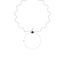
Figure 1: Two loop contribution to $\langle\Omega|F_{\mu\nu}(x)F_{\rho\sigma}(x)|\Omega\rangle$.

Passive fields can also induce interactions between active fields. For example, the photon loop in Fig. 2 induces an effective $(\varphi^{*}\varphi)^{2}$ interaction in SQED.

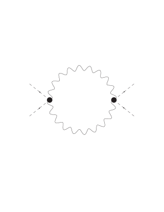
Figure 2: Effective $(\varphi^{*}\varphi)^{2}$ coupling in SQED.

In generalizing Starobinskiĭ’s technique to theories which include passive fields, it is crucial to realize that the ultraviolet parts of passive fields fields contribute on an equal footing with the infrared parts to the processes of propagating infrared logarithms and mediating interactions between active fields. So one cannot infrared truncate the passive fields. Instead the correct procedure is:

• Integrate out the passive fields and renormalize the resulting effective action; then

• Infrared truncate and stochastically simplify the purely active field effective action.

One might suspect that the second step is not possible owing to the nonlocality of the effective action. However, first note that VEV’s have no spatial dependence at leading logarithm order, so one can evaluate all fields at the same space point. It is still necessary to confront the prospect of fields buried inside different temporal integrals. However, precisely because they derive from passive fields, these temporal integrations always contain positive powers of the scale factor whose rapid time dependence weights the integral overwhelmingly at its upper limit and totally dominates the logarithms which might derive from the active fields.

As an example, consider the retarded Green’s function of a conformally coupled scalar,

$$G_{\rm cf}(x;x^{\prime})=\frac{H^{2}}{4\pi^{2}}\theta(\Delta t)\frac{\delta(H\Delta x+\frac{1}{a}-\frac{1}{a^{\prime}})}{aa^{\prime}H\Delta x}\;.$$ (41)

Acting this Green’s function on $\ln(a^{\prime})$ gives,

$$\int_{0}^{t}dt^{\prime}a^{\prime 3}\int d^{3}x^{\prime}G_{\rm cf}(x;x^{\prime})\times\ln(a^{\prime}) = \frac{1}{H}\int_{0}^{t}dt^{\prime}\Bigl{[}\frac{a^{\prime}}{a}-\Bigl{(}\frac{a^{\prime}}{a}\Bigr{)}^{2}\Bigr{]}\ln(a^{\prime})\;,$$ (42)

$$= \frac{1}{2H^{2}}\Bigl{\{}\ln(a)-\frac{3}{2}+\frac{2}{a}-\frac{1}{2a^{2}}\Bigr{\}}\;.$$ (43)

(To appreciate the distinction between the Green’s functions of passive and active fields, contrast (42) with (30).) On the other hand, the result of simply multiplying $\ln(a)$ by the Green’s function acted upon unity is,

$$\ln(a)\times\int_{0}^{t}dt^{\prime}a^{\prime 3}\int d^{3}x^{\prime}G_{\rm cf}(x;x^{\prime})=\frac{\ln(a)}{2H^{2}}\Bigl{\{}1-\frac{2}{a}+\frac{1}{a^{2}}\Bigr{\}}\;.$$ (44)

These expressions agree at leading logarithm order, so one may as well locate all the scalar fields at the same point and evaluate the inverse differential operators on unity. But that is just the same thing as computing the effective potential! Hence the hopelessly complicated “effective action” degenerates, in the leading log approximation, to a very tractable “effective potential,” and the resulting local theory assumes the form (21) already solved by Starobinskiĭ [23, 24].

This program has been carried out for SQED in collaboration with Nikolaos Tsamis and Tomislav Prokopec [29]. The various results are best expressed in terms of the following quantity,

$$z\equiv\frac{e^{2}\varphi^{*}\varphi}{H^{2}}\;.$$ (45)

If one renormalizes to make the quadratic and quartic terms of the effective potential vanish, the result is,

$$V_{\rm eff}=\frac{3H^{4}}{8\pi^{2}}\Biggl{\{}\Bigl{(}-1\!+\!2\gamma\Bigr{)}z+\Bigl{(}-\frac{3}{2}\!+\!\gamma\Bigr{)}z^{2}+\int_{0}^{z}dx(1\!+\!x)\Bigl{[}\psi(2\!-\!\Delta\nu_{0})+\psi(1\!+\!\Delta\nu_{0})\Bigr{]}\Biggr{\}}\;.$$ (46)

Here the function $\Delta\nu_{0}(x)$ is,

$$\Delta\nu_{0}(x)\equiv\frac{1}{2}-\frac{1}{2}\sqrt{1\!-\!8x}=2x+4x^{2}+8x^{3}+O(x^{4})\;,$$ (47)

and the PolyGamma function is,

$$\psi(1\!+\!z)\equiv\frac{d}{dz}\ln\Bigl{(}\Gamma(1\!+\!z)\Bigr{)}=-\gamma+\sum_{n=2}^{\infty}(-1)^{n}\zeta(n)z^{n-1}\;.$$ (48)

The effective potential of SQED in de Sitter background does not seem to have been computed previously. However, the $H=0$ limit of expression (46) agrees with equation (4.5) of Coleman and Weinberg [30].

To evaluate the VEV of any operator, one first integrates out the passive fields and stochastically simplifies the resulting, purely active field functional. One then computes the VEV using Starobinskiĭ’s formalism. Because the ultraviolet contributes for passive fields, the VEV’s of some operators are ultraviolet divergent even at leading logarithm order. The scalar functional resulting from the $D$-dimensionally regulated field strength bilinear is,

$$F_{\mu\nu}(x)F_{\rho\sigma}(x)\longrightarrow\Bigl{(}g_{\mu\rho}g_{\nu\sigma}-g_{\mu\sigma}g_{\nu\rho}\Bigr{)}\times\frac{H^{D}}{(4\pi)^{\frac{D}{2}}}\frac{\Gamma(\frac{D}{2}\!-\!1)\Gamma(2\!-\!\frac{D}{2})}{\Gamma(\frac{D}{2}\!+\!1)}\frac{\Gamma(\frac{D+1}{2}\!+\!\nu)\Gamma(\frac{D+1}{2}\!-\!\nu)}{\Gamma(\frac{1}{2}\!+\!\nu)\Gamma(\frac{1}{2}\!-\!\nu)}\;.$$ (49)

Here the scalar-dependent parameter $\nu(z)$ is,

$$\nu(z)\equiv\sqrt{\Bigl{(}\frac{D-3}{2}\Bigr{)}^{2}-2z}\equiv\Bigl{(}\frac{D-3}{2}\Bigr{)}-\Delta\nu(z)\;.$$ (50)

The analogous result for the scalar kinetic term is,

$$\Bigl{(}\partial_{\mu}\varphi^{*}(x)-ieA_{\mu}(x)\varphi^{*}(x)\Bigr{)}\Bigl{(}\partial_{\nu}\varphi(x)+ieA_{\nu}(x)\varphi(x)\Bigr{)}$$ (51)

$$\longrightarrow-\frac{1}{4}(D\!-\!1)g_{\mu\nu}\times\frac{H^{D}}{(4\pi)^{\frac{D}{2}}}\Biggl{\{}\frac{\Gamma(\frac{D}{2}\!-\!1)\Gamma(2\!-\!\frac{D}{2})}{\Gamma(\frac{D}{2}\!+\!1)}\frac{\Gamma(\frac{D+1}{2}\!+\!\nu)\Gamma(\frac{D+1}{2}\!-\!\nu)}{\Gamma(\frac{1}{2}\!+\!\nu)\Gamma(\frac{1}{2}\!-\!\nu)}-\frac{\Gamma(D\!-\!1)}{\Gamma(\frac{D}{2}\!+\!1)}\Biggr{\}}.\qquad$$

The leading logarithm result for the stress tensor is finite and takes the form $-g_{\mu\nu}V_{s}(z)$ where,

$$V_{\rm s}=\frac{3H^{4}}{16\pi^{2}}\Biggl{\{}\Bigl{(}-2\!+\!2\gamma\Bigr{)}z+\Bigl{(}-\frac{7}{2}\!+\!2\gamma\Bigr{)}z^{2}+z(1\!+\!z)\Bigl{[}\psi(1\!-\!2\Delta\nu_{0})+\psi(1\!+\!\Delta\nu_{0})\Bigr{]}\Biggr{\}}.$$ (52)

The stochastic prediction for (51) has been checked by an explicit two loop computation [31]. The predictions for (51) and (52) are still being checked.

In collaboration with Shun-Pei Miao, Starobinskiĭ’s formalism has also been applied to a massless, minimally coupled scalar which is Yukawa-coupled to a massless fermion [32]. The Lagrangian of this model is,

$$\mathcal{L}=-\frac{1}{2}\partial_{\alpha}\varphi\partial_{\beta}\varphi g^{\alpha\beta}\sqrt{-g}-\frac{1}{2}\delta\xi\varphi^{2}R\sqrt{-g}-\frac{1}{4!}\delta\lambda\varphi^{4}\sqrt{-g}+i\overline{\psi}e^{\beta}_{~{}b}\gamma^{b}{\cal D}_{\beta}\psi\sqrt{-g}-f\varphi\overline{\psi}\psi\sqrt{-g}\;,$$ (53)

where the spinor covariant derivative is,

$${\cal D}_{\mu}\equiv\partial_{\mu}+\frac{i}{2}A_{\mu cd}J^{cd}\;.$$ (54)

As with SQED, the conformal and quartic counterterms can be chosen to make the quadratic and quartic terms in the renormalized effective potential vanish. The final result is,

$$V_{\rm eff} = -\frac{H^{4}}{4\pi^{2}}\sum_{n=2}^{\infty}\frac{(-1)^{n}}{n\!+\!1}\Bigl{[}\zeta(2n\!-\!1)-\zeta(2n\!+\!1)\Bigr{]}\Bigl{(}\frac{f\varphi}{H}\Bigr{)}^{2n+2}\;,$$ (55)

$$= -\frac{H^{4}}{8\pi^{2}}\Biggl{\{}2\gamma\Bigl{(}\frac{f\varphi}{H}\Bigr{)}^{2}-[\zeta(3)\!-\!\gamma]\Bigl{(}\frac{f\varphi}{H}\Bigr{)}^{4}+2\int_{0}^{\frac{f\varphi}{H}}\!\!\!\!\!dx\,(x\!+\!x^{3})\Bigl{[}\psi(1\!+\!ix)\!+\!\psi(1\!-\!ix)\Bigr{]}\Biggr{\}}.\qquad$$ (56)

This agrees with the classic result of Candelas and Raine [33, 34, 35], and of course the $H=0$ limit agrees with equation (6.10) of Coleman and Weinberg [30, 36]. Note that this potential is unbounded below, which establishes that infrared logarithms need not always sum up to approach a static limit at late times.

As was the case for SQED, the leading logarithm result for the Yukawa stress tensor takes the form, $-g_{\mu\nu}V_{\rm s}(\varphi)$, where

$$V_{\rm s}(\varphi) = \frac{H^{4}}{8\pi^{2}}\Biggl{\{}\Bigl{[}\frac{1}{2}\!-\!\gamma\Bigr{]}\Bigl{(}\frac{f\varphi}{H}\Bigr{)}^{2}+\Bigl{[}\frac{1}{4}\!-\!\gamma\!+\!\zeta(3)\Bigr{]}\Bigl{(}\frac{f\varphi}{H}\Bigr{)}^{4}$$ (58)

$$\hskip 85.35826pt-\frac{1}{2}\Bigl{[}\Bigl{(}\frac{f\varphi}{H}\Bigr{)}^{2}\!+\!\Bigl{(}\frac{f\varphi}{H}\Bigr{)}^{4}\Bigr{]}\Bigl{[}\psi\Bigl{(}1\!+\!i\frac{f\varphi}{H}\Bigr{)}+\psi\Bigl{(}1\!-\!i\frac{f\varphi}{H}\Bigr{)}\Bigr{]}\Biggr{\}},$$

$$= \frac{H^{4}}{8\pi^{2}}\Biggl{\{}\frac{1}{2}\Bigl{(}\frac{f\varphi}{H}\Bigr{)}^{2}\!+\!\frac{1}{4}\Bigl{(}\frac{f\varphi}{H}\Bigr{)}^{4}\!-\!\sum_{n=2}^{\infty}(-1)^{n}\Bigl{[}\zeta(2n\!-\!1)\!-\!\zeta(2n\!+\!1)\Bigr{]}\Bigl{(}\frac{f\varphi}{H}\Bigr{)}^{2n+2}\Biggr{\}}.$$ (59)

The leading logarithm result for the dimensionally regulated coincident vertex function is,

$$\varphi(x)\overline{\psi}(x)\psi(x)\longrightarrow-4f\varphi^{2}(x)\frac{H^{D-2}}{(4\pi)^{\frac{D}{2}}}\Biggl{\|}\frac{\Gamma(\frac{D}{2}+\frac{if\varphi}{H})}{\Gamma(1+\frac{if\varphi}{H})}\Biggr{\|}^{2}\Gamma\Bigl{(}1\!-\!\frac{D}{2}\Bigr{)}\;.$$ (60)

Expression (60) was checked at order $f$ against an explicit two loop computation [32].

5 Other Geometries

Applying Starobinskiĭ’s formalism to more general theories on de Sitter background is essential to resolve the issue of what happens when infrared logarithms in these models become nonperturbatively strong. However, this does not suffice for extrapolating the enhanced quantum effects of these models to post-inflationary cosmology. For that it is necessary to understand how the effects manifest for a general scale factor $a(t)$. Two issues are of special importance:

• What becomes of the dependence upon the inflationary Hubble parameter $H$ which arises from integrating out passive fields?

• What becomes of the infrared logarithms generated by active fields?

Because the passive fields give local effects, it seems plausible that factors of $H$ generalize to local curvature scalars. The unique curvature scalar of dimension two is the Ricci scalar. Evaluating it respectively for a general scale factor and for de Sitter gives,

$$R_{\scriptscriptstyle{\rm FRW}}=12H^{2}(t)+6\dot{H}(t)\longrightarrow 12H^{2}\quad({\rm de\ Sitter})\;.$$ (61)

This suggests that factors of $H^{2}$ in de Sitter generalize to $R/12$. For example, the generalizations of the effective potentials of SQED (46) and Yukawa (56) would take the form,

$$V_{\scriptscriptstyle{\rm SQED}} = H^{4}F\Bigl{(}\frac{e^{2}\varphi^{*}\varphi}{H^{2}}\Bigr{)}\longrightarrow(\frac{1}{12}R)^{2}F\Bigl{(}\frac{12e^{2}\varphi^{*}\varphi}{R}\Bigr{)}\;,$$ (62)

$$V_{\scriptscriptstyle{\rm Yukawa}} = H^{4}G\Bigl{(}\frac{f^{2}\varphi^{2}}{H^{2}}\Bigr{)}\longrightarrow(\frac{1}{12}R)^{2}G\Bigl{(}\frac{12f^{2}\varphi^{2}}{R}\Bigr{)}\;.$$ (63)

It is presumably this additional dependence upon the metric which is responsible for the fact that the potentials of the leading logarithm stress tensors — expressions (52) and (58) — do not agree with the effective potentials (46) and (56). Note also that the putative generalization produces a curious sort of $R^{2}f(\varphi^{2}/R)$ model which may itself have cosmological significance.

Even in de Sitter, infrared logarithms measure the time since the onset of inflation, so they cannot generalize to a local invariant. One way of inferring the nonlocal invariant to which they generalize is to consider the expectation value of the square of a free, massless, and minimally coupled scalar for an arbitrary scale factor. Because the result is ultraviolet divergent, it must be regulated, although the generalized infrared logarithm should be finite. If the general $a(t)$ mode function is denoted $u[a](t,k)$, the result can be written as follows,

$$\Bigl{\langle}\Omega_{0}\Bigl{|}\varphi_{0}^{2}(t,\vec{x})\Bigr{|}\Omega_{0}\Bigr{\rangle}=\int\frac{d^{D-1}k}{(2\pi)^{D-1}}\Bigl{\|}u[a](t,k)\Bigr{\|}^{2}=\frac{2}{(4\pi)^{\frac{D-1}{2}}\Gamma(\frac{D-1}{2})}\int_{H}^{\infty}dkk^{D-2}\Bigl{\|}u[a](t,k)\Bigr{\|}^{2}\;.$$ (64)

Explicit expressions for $u[a](t,k)$ exist [2, 37]. Although these expressions are very complicated, the leading time dependence of (64) can perhaps be extracted.

6 Discussion

There is no question that infrared logarithms arise in explicit perturbative computations in many inflationary quantum field theories which involve MMC scalars and/or gravitons [5, 6, 7, 8, 9, 10, 11, 15, 16, 17, 18, 21, 20, 22]. These infrared logarithms counteract the small coupling constants which would otherwise suppress quantum loop effects. Over a long period of inflation they become so large that weak field perturbation theory breaks down. When the series of leading infrared logarithms is summed using Starobinskiĭ’s formalism, the result is that MMC scalars always reach nonperturbatively large field strengths. In the case of Yukawa theory the scalar grows without bound and comes to dominate late time cosmology [32]. It is not yet known what the nonperturbative outcome is for quantum gravity.

These enhanced quantum effects are not restricted to the MMC scalars and gravitons which cause them. Other fields seem to experience the following effects:

• Scalars with nonderivative couplings induce growing masses [5, 6, 7, 8, 9, 15]; and

• Gravitons and scalars with derivative couplings seem to induce changing field strengths [18, 22].

The now-established fact of significant, nonperturbative quantum effects from MMC scalars, and the prospect for them from gravitons, change the inflationary paradigm. Four processes occur which are absent in classical inflation:

• Certain field strengths reach nonperturbatively large values ($\sim H/{\rm coupling\ const}$);

• Inflation-induced masses engender a significant amount of vacuum energy which is positive for vector bosons and negative for fermions;

• The effective action of gravity suffers modifications of the form $\Delta{\cal L}=R^{2}f(\varphi^{2}/R)$; and

• A potentially significant amount of negative vacuum energy derives from the self-gravitation of inflationary gravitons.

Each of these processes can produce observable signals:

• Evolving scalars can induce resonant particle production [38];

• Vaccum energy from (Hubble scale) particle masses can serve as a reservoir for the creation of a vast population of cosmological wavelength vectors [39, 40, 41] and fermions when the mass dissipates after second horizon crossing;

• Modifications of gravity can change cosmology [42, 43]; and

• It is conceivable that inflation was caused by a bare, GUT-scale cosmological constant which is being screened by infrared quantum gravitational effects that became strong during primordial inflation [44].

The report covers work done jointly with Shun-Pei Miao, Tomislav Prokopec and Nikolaos Tsamis. I am also grateful for discussions and correspondence with Bjoern Garbrecht and Pei-Ming Ho. This work was partially supported by NSF grant PHY-0244714 and by the Institute for Fundamental Theory at the University of Florida.

References

References

- [1] R. P. Woodard, “Fermion Self-Energy during Inflation,” in XIIth International Conference on Selected Problems of Modern Physics, edited by B. M. Barbashov, G. V. Efimov, A. V. Efremov, S. M. Eliseev, V. V. Nesterenko and M. K. Volkov (JINR, Dubna, 2003), pp. 355-366, astro-ph/0307269.
- [2] N. C. Tsamis and R. P. Woodard, Class. Quant. Grav. 20 (2003) 5205, astro-ph/0206010.
- [3] V. F. Mukhanov and G. V. Chibisov, JETP Letters 33 (1981) 532.
- [4] A. A. Starobinskiĭ, JETP Letters 30 (1979) 682.
- [5] T. Prokopec, O. Tornkvist and R. P. Woodard, Phys. Rev. Lett. 89 (2002) 101301, astro-ph/0205331.
- [6] T. Prokopec, O. Tornkvist and R. P. Woodard, Ann. Phys. 303 (2003) 251, gr-qc/0205130.
- [7] T. Prokopec and R. P. Woodard, Ann. Phys. 312 (2204) 1, gr-qc/0310056.
- [8] T. Prokopec and R. P. Woodard, JHEP 0310 (2003) 059, astro-ph/0309593.
- [9] B. Garbrecht and T. Prokopec, Phys. Rev. D 73 (2006) 064036, gr-qc/0602011.
- [10] V. K. Onemli and R. P. Woodard, Class. Quant. Grav. 19 (2002) 4607, gr-qc/0204065.
- [11] V. K. Onemli and R. P. Woodard, Phys. Rev. D 70 (2004) 107301, gr-qc/0406098.
- [12] A. Vilenkin and L. H. Ford, Phys. Rev. D 26 (1982) 1231.
- [13] A. D. Linde, Phys. Lett. B 116 (1982) 335.
- [14] A. A. Starobinskiĭ, Phys. Lett. B 117 (1982) 175.
- [15] T. Brunier, V. K. Onemli and R. P. Woodard, Class. Quant. Grav. 22 (2005) 59, gr-qc/0408080.
- [16] N. C. Tsamis and R. P. Woodard, Phys. Rev. D 54 (1996) 2621, hep-ph/9602317.
- [17] N. C. Tsamis and R. P. Woodard, Ann. Phys. 253 (1997) 1, hep-ph/9602316.
- [18] S. Weinberg, Phys. Rev. D 72 (2005) 043514, 2005, hep-th/0506236.
- [19] M. Sloth, Nucl. Phys. B 748 (2006) 149, astro-ph/0604488.
- [20] S. Weinberg, Phys. Rev. D74 (2006) 023508, hep-th/0605244.
- [21] S. P. Miao and R. P. Woodard, Class. Quant. Grav. 23 (2006) 1721, gr-qc/0511140.
- [22] S. P. Miao and R. P. Woodard, Phys. Rev. D 74 (2006) 024021, gr-qc/0603135.
- [23] A. A. Starobinskiĭ, “Stochastic de Sitter (inflationary) stage in the early universe,” in Field Theory, Quantum Gravity and Strings, edited by H. J. de Vega and N. Sanchez (Springer-Verlag, Berlin, 1986), pp. 107-126.
- [24] A. A. Starobinskiĭ and J. Yokoyama, Phys. Rev. D 50 (1994) 6357, astro-ph/9407016.
- [25] R. P. Woodard, Nucl. Phys. Proc. Suppl. 148 (2005) 108, astro-ph/0502556.
- [26] N. C. Tsamis and R. P. Woodard, Nucl. Phys. B 724 (2005) 295, gr-qc/0505115.
- [27] C. N. Yang and D. Feldman, Phys. Rev. 79 (1950) 972.
- [28] L. Accardi, Y. G. Lu and I. Volovich, Quantum Theory and Its Stochastic Limit (Springer-Verlag, Berlin, 2002).
- [29] T. Prokopec, N. C. Tsamis and R. P. Woodard, Annals Phys. 323 (2008) 1324, arXiv:0707.0847.
- [30] S. R. Coleman and E. Weinberg, Phys. Rev. D 7 (1973) 1888.
- [31] T. Prokopec, N. C. Tsamis and R. P. Woodard, Class. Quant. Grav. 24 (2007) 201, gr-qc/0607094.
- [32] S. P. Miao and R. P. Woodard, Phys. Rev. D74 (2006) 044019, gr-qc/0602110.
- [33] P. Candelas and D. J. Raine, Phys. Rev. D 12 (1975) 965.
- [34] T. Inagaki, S. Mukaigawa and T. Muta, Phys. Rev. D 52 (1995) 4267, hep-th/9505058.
- [35] T. Inagaki, T. Muta and S. D. Odintsov, Prog. Theor. Phys. Suppl. 127 (1997) 93, hep-th/9711084.
- [36] B. Garbrecht, Phys. Rev. D74 (2006) 043507, hep-th/0604166.
- [37] N. C. Tsamis and R. P. Woodard, Class. Quant. Grav. 21 (2003) 93, astro-ph/0306602.
- [38] D. J. H. Chung, E. W. Kolb, A. Riotto and I. I. Tkachev, Phys. Rev. D 62 (2000) 043508, hep-ph/9910437.
- [39] A. C. Davis, K. Dimopoulos, T. Prokopec and O. Törnkvist, Phys. Lett. B 501 (2001) 165, astro-ph/0007214.
- [40] K. Dimopoulos, T. Prokopec, O. Törnkvist and A. C. Davis, Phys. Rev. D 65 (2002) 165, astro-ph/0108093.
- [41] T. Prokopec and R. P. Woodard, Am. J. Phys. 72 (2004) 60, astro-ph/0303358.
- [42] R. P. Woodard, Lect. Notes Phys. 720 (2007) 403, astro-ph/060167.
- [43] S. Nojiri and S. D. Odintsov, Int. J. Geom. Meth. Mod. Phys. 4 (2007) 115, hep-th/0601213.
- [44] N. C. Tsamis and R. P. Woodard, Nucl.Phys. B 474 (1996) 235, hep-ph/9602315.