Abstract

Measurement of gravitomagnetic field is of fundamental importance as a test of general relativity. Here we present a new theoretical project for performing such a measurement based on detection of the electric field arising from the interplay between the gravitomagnetic and magnetic fields in the stationary axial-symmetric gravitational field of a slowly rotating massive body. Finally it is shown that precise magnetometers based on superconducting quantum interferometers could not be designed for measurement of the gravitomagnetically induced magnetic field in the cavity of a charged capacitor since they measure the circulation of a vector potential of electromagnetic field, i.e., an invariant quantity including the sum of electric and magnetic fields, and the general-relativistic magnetic part will be totally cancelled by the electric one which is in good agreement with the experimental results.

KEY WORDS: Gravitomagnetism; general relativity; Lense-Thirring effect

1 Introduction

General relativity predicts that a spinning central massive body creates a gravitomagnetic field in addition to the Newtonian-like monopolar gravitoelectric one, that is static gravitational mass generates solely gravitoelectric field and a moving body, an additional gravitomagnetic one as in electrodynamics (see, for review,  [1]). Almost all the classical tests of general relativity (gravitational redshift, perihelion precession of Mercury, gravitational deflection of light) confirm the validity of the general-relativistic corrections to the Newtonian gravitoelectric field with high accuracy. But due to the weakness of the gravitomagnetic field in the Solar system it is very hard to detect it although many theoretical projects on measuring gravitomagnetism have been proposed  [1].

In our recent papers [2, 3] the gravitomagnetic effect on the electric current and magnetic field has been investigated on the theoretical level. In fact, the influence of the angular momentum of the rotating gravitational source may appear as a galvanogravitomagnetic effect in the current carrying conductors [2] and as a general-relativistic effect of charge redistribution inside conductors in an applied magnetic field  [3]. It is natural to ask whether the gravitomagnetic interaction with electric field can lead to the applicable general-relativistic effects. Our aim here is to investigate an answer to this question and present a new measurement scheme which could lead to a detection of the earth’s gravitomagnetic field in the electromagnetic systems.

The paper is organized as follows: in section 2 we deal with electromagnetic fields in both the cavity of charged capacitor and solenoid embedded in a space-time of slow rotating gravitational object. The next section 3 is devoted to a proposal for measuring gravitomagnetic field in the electromagnetic systems. In section 4 we discuss the impossibility of detection of gravitomagnetic field through direct measurement of a gravitomagnetically induced magnetic field in the cavity of charged capacitor. Finally section 5 contains concluding remarks.

2 Electromagnetic fields in electromagnetic systems in space-time of rotating object

Consider first electromagnetic fields inside the charged capacitor in the stationary axial-symmetric metric of a slowly rotating massive body as the earth. Space-time outside a spherically symmetric mass $M$ with the specific angular momentum $a=J/(cM)$ is described by the Kerr metric [4]. This differs from the Schwarzschild solution for a static body by having non-diagonal terms, which imply a local inertial frame to be rotating with respect to the distant stars at infinity with the Lense-Thirring angular velocity $\omega(r)\equiv{2aGM}/{c^{2}r^{3}}$ [5]. Then the exterior metric of the slow rotating gravitational object with mass $M$ (in the linear angular momentum $a$ approximation) is

$$ds^{2}=-N^{2}c^{2}dt^{2}+N^{-2}dr^{2}+r^{2}d\theta^{2}+r^{2}\sin{}^{2}\theta d\varphi^{2}-2{{\omega}}r^{2}\sin{}^{2}\theta dtd\varphi\ ,$$ (1)

where $N\equiv\left({1-{2GM}/{\left(c^{2}r\right)}}\right)^{1/2}$, $G$ is the Newtonian gravitational constant. Thus the angular velocity of the body as measured from the local free falling (inertial) observer is ${\bar{\omega}}\equiv\Omega-\omega(r)$, $\Omega$ is angular velocity of rotation of gravitational object with respect to the distant stars.

Define the electric and magnetic fields relative to an observer with four-velocity $e^{\alpha}\equiv{dx^{\alpha}}/{d\tau}$ ($d\tau$ is its proper time) as

$$E_{\alpha}=F_{\alpha\beta}e^{\beta}\ ,\qquad B_{\alpha}=-\frac{1}{2}e_{\alpha\beta\mu\nu}e^{\beta}F^{\mu\nu}\ ,$$ (2)

where $e_{\alpha\beta\mu\nu}$ is the antisymmetric pseudo-tensorial expression of the Levi-Civita symbol $\epsilon_{\alpha\beta\mu\nu}$, $F_{\alpha\beta}=A_{\beta,\alpha}-A_{\alpha,\beta}$ and $A_{\alpha}$ are the tensor and four-potential of electromagnetic field, respectively. Greek indices run through $0,1,2,3$ and Latin indices from $1$ to $3$.

Element of an arbitrary 2-surface $dS^{\alpha\beta}$ can be represented in the form

$$dS^{\alpha\beta}=-e^{\alpha}\wedge m^{\beta}(ek)dS+e^{\alpha\beta\mu\nu}e_{\mu}n_{\nu}\sqrt{1+(ek)^{2}}dS\ ,$$ (3)

and the following couples

$$m_{\alpha}=\frac{e_{\lambda\alpha\mu\nu}e^{\lambda}n^{\mu}k^{\nu}}{\sqrt{1+(ek)^{2}}},n_{\alpha}=\frac{e_{\lambda\alpha\mu\nu}e^{\lambda}k^{\mu}m^{\nu}}{\sqrt{1+(ek)^{2}}},k^{\alpha}=-(ek)e^{\alpha}+\sqrt{1+(ek)^{2}}e^{\mu\alpha\rho\nu}e_{\mu}m_{\rho}n_{\nu}$$

are established between the triple $\{{\mathbf{k}},{\mathbf{m}},{\mathbf{n}}\}$ of vectors, $n^{\alpha}$ is normal to 2-surface, space-like vector $m^{\alpha}$ belongs to the given 2-surface and is orthogonal to the four-velocity of observer, a unit spacelike four-vector $k^{\alpha}$ belongs to the surface and is orthogonal to $m^{\alpha}$, $dS$ is invariant element of surface.

At the two-dimentional surface an arbitrary pair of mutually orthogonal vectors $\{{\mathbf{t}},{\mathbf{s}}\}$ can be expressed through pair $\{{\mathbf{k}},{\mathbf{m}}\}$ in the following way

$$t^{\alpha}=\cos\varphi k^{\alpha}+\sin\varphi m^{\alpha},\qquad s^{\alpha}=\cos\varphi m^{\alpha}+\sin\varphi k^{\alpha}\ .$$

Let a charged capacitor with the opposite surface density of charges $\sigma_{s}$ at the plates be at rest in space-time (1); a constant charge is supplied by a battery of constant electromotive force. Then the boundary conditions for the jumps $[X]$ of the electromagnetic fields $E^{\alpha},B^{\alpha}$ and inductions $D^{\alpha},H^{\alpha}$ at the plates being the pieces of the coordinate surfaces take form:

$$(n1) \qquad[Bn]=0,\qquad(n2)\qquad[Dn]=4\pi\sigma_{s}\sqrt{1+(ek)^{2}}\ ,$$ (4)

$$(t1) \qquad[Et]=0,\qquad(t2)\qquad[Ht]=4\pi\sigma_{s}(ek)\sin\varphi\ .$$

The electromagnetic fields could be written in an orthonormal frame with the tetrad $\{{\bf e}_{\hat{\mu}}\}=({\bf e}_{\hat{0}},{\bf e}_{\hat{r}},{\bf e}_{\hat{\theta}},{\bf e}_{\hat{\phi}})$

$${\bf e}_{\hat{0}}^{\alpha}=N^{-1}\bigg{(}1,0,0,{\omega}\bigg{)}\ ,$$ (5)

$${\bf e}_{\hat{r}}^{\alpha}=N\bigg{(}0,1,0,0\bigg{)}\ ,$$ (6)

$${\bf e}_{\hat{\theta}}^{\alpha}=\frac{1}{r}\bigg{(}0,0,1,0\bigg{)}\ ,$$ (7)

$${\bf e}_{\hat{\phi}}^{\alpha}=\frac{1}{r\sin\theta}\bigg{(}0,0,0,1\bigg{)}\ .$$ (8)

The 1-forms $\{{\bf\omega}^{\hat{\mu}}\}=({\bf\omega}^{\hat{0}},{\bf\omega}^{\hat{r}},{\bf\omega}^{\hat{\theta}},{\bf\omega}^{\hat{\phi}})$, corresponding to this tetrad are

$${\bf\omega}^{\hat{0}}_{\alpha}=N\bigg{(}1,0,0,0\bigg{)}\ ,$$ (9)

$${\bf\omega}^{\hat{r}}_{\alpha}=N^{-1}\bigg{(}0,1,0,0\bigg{)}\ ,$$ (10)

$${\bf\omega}^{\hat{\theta}}_{\alpha}={r}\bigg{(}0,0,1,0\bigg{)}\ ,$$ (11)

$${\bf\omega}^{\hat{\phi}}_{\alpha}={r\sin\theta}\bigg{(}-{\omega},0,0,1\bigg{)}\ .$$ (12)

Suppose that the plates of capacitor are pieces of the coordinate surfaces $r=const.$ with the characteristic vectors

$$k^{\alpha}\{0,0,0,\frac{1}{r\sin\theta}\}\ ,\quad m^{\alpha}\{0,0,-\frac{1}{r},0\}\ ,\quad n^{\alpha}\{0,{N},0,0\}\ ,$$ (13)

where the boundary conditions (4) take the form

$$[B^{\hat{r}}]=[E^{\hat{\theta}}]=[E^{\hat{\phi}}]=[H^{\hat{\phi}}] = 0,$$

$${[D^{\hat{r}}]}=4\pi\sigma_{s}{N}^{-1}|_{r=const},\qquad[H^{\hat{\theta}}] = 4\pi\sigma_{s}N^{-1}\frac{\omega r\sin\theta}{c}|_{r=const}\ .$$ (14)

Due to the axial symmetry and stationarity of the problem the field vectors depend on the space coordinates $r$ and $\theta$. If there is the potential difference $\Delta\phi\equiv\Delta A_{0}$ between the plates of capacitor $r=r_{1}$ and $r=r_{2}$ ($\Delta r=r_{2}-r_{1}$) then nonvanishing components of the electromagnetic field are defined by the formulae:

$$E^{\hat{r}}=\frac{\Delta\phi}{\Delta r}N^{-1},\quad B^{\hat{\theta}}=\frac{\omega r\sin\theta}{c}\frac{\Delta\phi}{\Delta r}N^{-1}\ .$$ (15)

As one can see the electric field in the metric (1) is modified by the coupling to the static monopolar part of gravitational field defined by the mass $M$ while the magnetic field is generated due to the interplay between the dragging of inertial frames and electric field, and vanishes in the Schwarzschild space-time.

Consider now electromagnetic fields outside infinitely long solenoid carrying constant electric current. It has been recently shown (see, for example, [10, 11]) that the electric field being proportional to $(\omega r/c)B$ is induced in a slowly rotating metric (1) of a star with magnetic field $B$. Analogously one can expect that in the linear approximation in the angular velocity of rotation the electric field

$$E\approx(\omega r/c)B$$ (16)

is induced around the solenoid carrying constant current.

3 Feasibility of an experiment on measuring gravitomagnetism

It is well-known that the electric field induced by gravity was first detected in [6, 7, 8] by analyzing the time-of-flight distribution of electrons falling freely within a metal cylindrical hollow tube (with the length $L$) where the electrons experienced the force of gravity $mg$ ($g$ is the gravitational acceleration), the gravitoelectrically induced electric field $E_{i}$ and an applied weak uniform electric field $E_{a}$. By measuring the maximum observable flight time of electrons

$$t_{max}=[2Lm/(mg-eE_{i}+eE_{a})]^{1/2}$$ (17)

for several values of $E_{a}$, the experimental value for $E_{i}$ was obtained with high accuracy up to $10^{-11}-10^{-12}V/m$.

In the present paper a simple method for proposal on measuring gravitomagnetism is studied by assuming ideal experimental conditions. In order to grasp the idea, let us start from the equation of motion of charge $q$ with mass $m$ in electromagnetic and stationary gravitational field of a rotating mass (in the weak gravitational field and slow motion limit) [1]

$$m\frac{d{\mathbf{v}}}{dt}\cong q({\mathbf{E}}+\frac{1}{c}{\mathbf{v}}\times{\mathbf{B}})+m({\mathbf{E}}_{g}+\frac{1}{c}{\mathbf{v}}\times{\mathbf{B}}_{g})\ ,$$ (18)

where the gravitational field is decomposed into a “gravitoelectric” part

$${\mathbf{E}}_{g}=-\frac{GM}{r^{2}}\hat{\mathbf{r}}$$ (19)

and a “gravitomagnetic” one

$${\mathbf{B}}_{g}={\mathbf{\nabla}}\times{\mathbf{A}}_{g}=\frac{2G}{c}[\frac{({\mathbf{J}}-3({\mathbf{J}\cdot\hat{r}})\hat{\mathbf{r}})}{r^{3}}]\ ,$$ (20)

$\hat{\mathbf{r}}$ is the unit vector responsible for the position of test particle and the gravitomagnetic potential is given by

$${\mathbf{A}}_{g}=-\frac{2G}{c}\frac{{\mathbf{J}}\times{\mathbf{r}}}{r^{3}}\ .$$ (21)

In the frame $K\{x,y,z\}$ whose $(x,y)$-plane coincides with the equatorial plane of gravitating source its proper angular momentum is directed along the $z$- axis, ${\mathbf{J}}=J{\mathbf{i}}_{z}$ and the equation for the gravitomagnetic field ${\mathbf{B}}_{g}$ immediately yields

$${\mathbf{B}}_{g}=\frac{2G}{c}\frac{J}{R^{3}}{\mathbf{i}}_{z}\ .$$ (22)

The solution of the equation of motion (18) for a charged particle, when there is no gravity, in crossed constant electric and magnetic fields is well-known (see, for example, [9]). The crucial point for further analysis is that in the direction perpendicular to the common plane of fields $\mathbf{E}$ and $\mathbf{B}$, a particle moves with a velocity which is a periodic function of time, drift velocity

$${\mathbf{v}}_{drift}=\frac{{\mathbf{E}}\times{\mathbf{B}}}{B^{2}}\ .$$ (23)

In the particular cases i) ${\mathbf{B}}=0,{\mathbf{v}}_{drift}=0$ in the perpendicular direction (the motion only in the direction being parallel to electric field); ii) ${\mathbf{E}}=0,{\mathbf{v}}_{drift}=0$ and the orbit of the particle is a helix, with its axis parallel to magnetic field.

Thus according to equations (18) and (15) the motion of electrons in the vicinity of the solenoid carrying constant electric current will be effected by the gravitoelectric field and gravitomagnetically induced electric field. The investigation of the electron motion in the vicinity of the solenoid can give a successful method to detect the gravitomagnetic field of the earth. The essential part of the suggested method could be based on the gravitomagnetical generation of electric field crossed to the original magnetic one.

Now let us have a look at figure. The magnetic field $B^{\hat{\alpha}}\{0,0,B\}$ is along the horizontal $z$ axis and gravitomagnetically induced electric field (16) $E^{\hat{\alpha}}\{0,(\omega R/c)B,0\}$ is along the vertical $y$ axis. The particle moves in the $z$ direction with a uniform velocity. Then in the coordinate system $K(x,y,z)$, the equation of motion of charged particle reads

$$m\frac{d{\mathbf{v}}}{dt}=m{\mathbf{E}}_{g}+q{\mathbf{E}}+q{\mathbf{v}}\times{\mathbf{B}}_{t}\ ,$$ (24)

with the gravitoelectric field, velocity and electromagnetic field given by

$${\mathbf{E}}_{g} = g{\mathbf{j}}\ ,\qquad{\mathbf{v}}=\dot{x}{\mathbf{i}}+\dot{y}{\mathbf{j}}+\dot{z}{\mathbf{k}}\ ,$$

$${\mathbf{E}} = E_{x}{\mathbf{i}}+E_{y}{\mathbf{j}}+E_{z}{\mathbf{k}}\ ,\qquad{\mathbf{B}}=B_{t}{\mathbf{k}}\ ,\qquad B_{t}=B+\frac{m}{q}B_{g}\ ,$$ (25)

where ${\mathbf{i}},{\mathbf{j}}$ and ${\mathbf{k}}$ are unit vectors along the corresponding rectangular axes (see Figure 1).

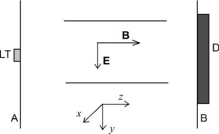
Figure 1: Scheme of proposed experiment. $D$ is the detector, ${\mathbf{B}}$ is the magnetic field, ${\mathbf{E}}$ is the electric field.

Using the equation of motion (24) and (3) a very simple calculation leads to the system of equations

$$\frac{d}{dt}\left(\dot{x}+i\dot{y}\right)+\frac{qB_{t}}{m}\left(\dot{x}+i\dot{y}\right)=\frac{q}{m}\left(E_{x}+iE_{y}\right)+ig\ ,$$ (26)

$$\ddot{z}=\frac{q}{m}E_{z}\ .$$

It is an ideal case to have $E_{x}=E_{y}=0$ in the system (26). However there are always small stray electric fields (In a superconducting drift tube as demonstrated by Witteborn and Fairbank [6], stray electric fields could be controlled at the level of $10^{-11}V/m$.).

In the real experimental situation a confining electric field can be produced. We shall also include some small constant stray fields $e^{\hat{i}}\{e_{x},e_{y},e_{z}\}$, so that for electric field in the system (26) we have

$$E_{x}=-c_{1}z-e_{x}\ ,\qquad E_{y}=-c_{2}z-e_{y}\ ,\qquad E_{z}=-c_{3}z-e_{z}\ .$$ (27)

Introducing electric field (27) into (26) gives

$$\frac{dv}{dt}+i\Omega_{L}v=-\frac{q}{m}\left(c_{1}+ic_{2}\right)z-\frac{q}{m}\left(e_{x}+ie_{y}\right)+ig\ ,$$ (28)

$$\ddot{z}+\Omega_{0}^{2}z=-\frac{q}{m}\$$

with

$$\Omega_{L}=\frac{qB_{t}}{m}\ ,\qquad\Omega_{0}^{2}=\frac{qc_{3}}{m}\ ,\qquad v=\left(\dot{x}+i\dot{y}\right)\ .$$ (29)

The general solution of the equation (LABEL:system2) is

$$z=C_{1}\sin\left(\Omega_{0}t+\varphi\right)-\frac{e_{z}}{c_{3}}\$$ (30)

and charge oscillates along $z$ axis. Here $C_{1}$ and $\varphi$ are integration constants depending on boundary conditions. According to the solution (30), the equation (28) can be written as

$$\frac{dv}{dt}+i\Omega_{L}v=-A\sin\left(\Omega_{0}t+\varphi\right)+B_{t}+ig\ ,$$ (31)

with

$$A=C_{1}\frac{q}{m}\left(c_{1}+ic_{2}\right)\ ,\qquad B_{t}=\frac{q}{m}\left(-\left(e_{x}+ie_{y}\right)+\frac{e_{z}}{c_{3}}\left(c_{1}+ic_{2}\right)\right)\ .$$ (32)

The solution of equation (31) is

$$v=-\frac{A}{\Omega_{L}(1-\Omega_{0}^{2}/\Omega_{L}^{2})}\left(\frac{\Omega_{0}}{\Omega_{L}}\cos\left(\Omega_{0}t+\varphi\right)-i\sin\left(\Omega_{0}t+\varphi\right)\right)+\frac{a}{\Omega_{L}}+\frac{B_{t}}{i\Omega_{L}}+C_{2}e^{-i\Omega_{L}t}\ .$$ (33)

As a consequence of (33), $\dot{x}$ and $\dot{y}$ are the periodic functions of time with average values

$$\bar{\dot{x}}=\frac{a}{\Omega_{L}}+\frac{q}{m\Omega_{L}}\left(\frac{e_{z}}{c_{3}}c_{2}-e_{y}\right)\quad\bar{\dot{y}}=\frac{q}{m\Omega_{L}}\left(\frac{e_{z}}{c_{3}}c_{1}-e_{x}\right)\ .$$ (34)

In the case when stray electric fields $e^{\hat{i}}=0$ vanish, the solution (33) becomes very simple:

$$\bar{\dot{x}}=\frac{a}{\Omega_{L}}\qquad and\qquad\bar{\dot{y}}=0\ .$$ (35)

With a good control of stray fields as in paper [7] drift along the $x$ axis caused by field (16) could be measured.

4 On direct measurement of gravitomagnetically induced electromagnetic field

It should be mentioned that the question of direct measurement of gravitomagnetically generated magnetic field has been experimentally tested [12] and the null result of the experiment was treated as a verification of the principle of equivalence.

In experiment [12] superconducting quantum interferometers (SQUIDs) have been used in order to detect the magnetic field generated by the gravitomagnetic effect on electric field, i.e. to measure magnetic field inside charged capacitor embedded in the earth’s gravitational field under the different space orientations of the equipment. The original idea of experiment [12] was based on the following two main assumptions.

First, the constitutive relations [9]

$${\mathbf{B}}=\frac{\mu{\mathbf{H}}}{\sqrt{-g_{00}}}+({\mathbf{g}}\times{\mathbf{E}}),\qquad{\mathbf{D}}=\frac{\epsilon{\mathbf{E}}}{\sqrt{-g_{00}}}-({\mathbf{g}}\times{\mathbf{H}})$$ (36)

between the electromagnetic fields and inductions for isotropic media with dielectric permittivity $\epsilon$ and the magnetic permeability $\mu$ lead to the assumption that under the influence of the dynamical gravitomagnetic part $g_{\alpha}\{0,{g_{0i}}/{\sqrt{-g_{00}}}\}$ of the gravitational field on electromagnetic phenomena a magnetic field will be induced by the stationary electric field and vice versa.

Second, a SQUID was expected to measure the flux of magnetic induction $\int{\mathbf{B}}d{\mathbf{S}}$ in general relativistic case as in the flat space-time, that is the standard electromagnetic result according to which a SQUID measures the flux of a magnetic field was applied to the treatment in the space-time of rotating gravitational object.

Assuming the earth in the first approximation is slowly rotating gravitational body  and using these two prepositions the authors [12] expected that SQUID should detect the nonvanishing gravitomagnetically generated quantity $\int({\mathbf{g}}\times{\mathbf{E}})d{\mathbf{S}}$ inside the charged capacitor located on the earth. However, a number of measurements of the magnetic flux inside the charged capacitor on the earth did not give positive result. It was established experimentally that the quantity measured by the SQUID inside the condenser does not depend on the space orientation of the equipment with respect to the distant stars.

In order to show that null experiment [12] can be predicted in the framework of the general-relativistic electrodynamics of continuous media it is necessary to get an answer to two important questions: (i) which quantity is measured by the SQUID embedded in external gravitational field and (ii) how the measuring quantity corresponds to the electromagnetic fields generated in the cavity of the charged capacitor.

In order to get a solution to the first question we consider the general-relativistic generalization of the Bohr-Sommerfeld quantization condition for the Cooper pairs

$$\oint_{\gamma}p_{\alpha}dx^{\alpha}=\oint_{\gamma}(2mcu_{(s)\alpha}+\frac{2e}{c}A_{\alpha})dx^{\alpha}=n\hbar\ ,$$ (37)

which is the macroscopic analog of the quantization of angular momentum $p_{\alpha}$ in an atomic system. Here $n$ is an integer, $\hbar$ is the Planck’s constant, $\gamma$ is a closed curve in the interior of superconductor, $u_{(s)\alpha}$ is the four-velocity of the Cooper pairs.

Using the Stokes theorem [13] we can extend the integration over the surface $dS^{\alpha\beta}$ spanned by the curve. Then condition (37) may be rewritten in the form

$$\frac{mc^{2}/e}{\sqrt{1-v_{(s)}^{2}/c^{2}}}\int A_{\alpha\beta}dS^{\alpha\beta}+\Lambda^{-1}c\oint\hat{\jmath}_{(s)\alpha}dx^{\alpha}+\frac{1}{2}\int F_{\alpha\beta}dS^{\alpha\beta}=n\Phi_{0}\ ,$$ (38)

which asserts, due to nonpenetration of the superconducting current into the bulk of the superconductor, that the sum of flux of the electromagnetic tensor and the purely relativistic term arising from the rate of rotation $2A_{\beta\alpha}=u_{\alpha,\beta}-u_{\beta,\alpha}+u_{\beta}\wedge w_{\alpha}$ is quantized in the general-relativistic context (the general-relativistic contribution leads to the relativistic London moment [14]-[16]). Here $\Phi_{0}={\hbar c}/{2e}$ is the flux quantum, $\hat{\jmath}^{\alpha}_{(s)}$ is the superconducting current, $v^{\alpha}_{(s)}$ is the velocity of superconducting electrons relative to the medium as a whole with the four-velocity $u^{\alpha}$ and the absolute acceleration $w_{\alpha}=u_{\alpha;\beta}u^{\beta}$, $\wedge$ is the symbol of exterior product.

Thus the superconducting quantum interferometers are adjusted for measurement of circulation of the 4-potential of electromagnetic field along the closed contour

$$\Phi_{B}=\oint A_{\alpha}dx^{\alpha}=\frac{1}{2}\int F_{\alpha\beta}dS^{\alpha\beta}\ ,$$ (39)

and consequently the SQUID in principle measures the flux of electromagnetic field tensor $F_{\alpha\beta}$ (rather the flux of magnetic field as expected in [12]) which is defined in an invariant way and does not explicitly depend on an observer.

Magnetic flux (39) through the surface of a measuring contour may be nonvanishing only if it contains the projection on the surface $\theta=const$ with the characteristic vectors

$$k^{\alpha}\{0,0,0,\frac{1}{r\sin\theta}\},\quad m^{\alpha}\{0,N,0,0\},\quad n^{\alpha}\{0,0,\frac{1}{r},0\}\ .$$ (40)

Then having in mind (2), (15) and (3) we obtain

$$\Phi_{B}=\int B_{\alpha}n^{\alpha}\sqrt{1+(ek)^{2}}dS+\int E_{\alpha}m^{\alpha}(ek)dS=$$

$$\frac{1}{c}\int(\Delta\phi/\Delta r)N^{-1}\omega\sin\theta dS-\frac{1}{c}\int(\Delta\phi/\Delta r)N^{-1}\omega\sin\theta dS\equiv 0\ .$$ (41)

Similarly one may show that the value of the flux of electromagnetic tensor (39) through the surface of measuring loop inside the charged capacitor is equal to zero for any other space orientations of equipment in the axisymmetric space-time geometry (1). Thus the total flux inside the capacitor being independent of its orientation is in the agreement with the null result of the treated experiment [12] (unlike Vasil’ev’s [12] treatmeant of the null result as a consequence of absence of the gravitatomagnetic effects on the electromagnetic processes according to the principle of equivalence) which indirectly confirms that the magnetic field can be created inside the capacitor by the interplay between electric and gravitomagnetic fields. It appears the SQUID measures the invariant flux (4) including contribution from the electric field and consequently the contribution due to the general-relativistic gravitomagnetic effect, i.e., the second term on the right hand side of (4) is totally cancelled by the first term in the process of the measurement. It should be noted the obtained result could be considered as a consequence of (39) when the four-potential $A_{\alpha}\{A_{0},0,0,0\}$ of electromagnetic field has only nonvanishing component $A_{0}\neq 0$.

Consider now a possibility to detect the gravitomagnetic field in the space of the solenoid with constant electric current. It is known that the constant magnetic field in a slowly rotating metric (1) is modified by the gravitoelectric factor but has no any contribution from the gravitomagnetic field (see, for example, [10, 11]). In the linear approximation in the angular velocity of rotation magnetic flux (39) around the solenoid carrying constant current is defined only by the magnetic field since the term produced by the electric field in (39) is proportional to $O(\omega^{2})$ and therefore negligible. So the gravitomagnetic field can not be detected via the direct measurement of the elecromagnetic field around solenoid by superconducting loop although it can be tested via the general-relativistic effect of charge redistribution inside a conductor embedded in the magnetic field of the solenoid [3]. Thus we can make a general conclusion that the direct SQUID’s measurements of the electromagnetic fields in the stationary conditions can not detect the gravitomagnetic field although in our recent paper [2] we have shown that the SQUID measuring the galvanogravitomagnetic current (not field) can be used as a detector of the gravitomagnetism.

5 Concluding remarks

As we have shown here, on one side, due to the gravitomagnetic effect, a magnetic field  (15) will be induced inside a cavity of condenser in addition to the electric one. On other side, the second term arising on the right hand side of the flux (4) totally compensates the gravitomagnetically induced magnetic field. In this sense the experiment [12] is analogous to the null result experiment [17] on test of the principle of equivalence for electromagnetic systems, where the gravitational redshift of the microwave frequency $\Delta\nu/\nu=\lambda$ was totally compensated by the general-relativistic effect due to the fact that the gravitoelectrochemical potential ${\tilde{\mu_{e}}}=\mu_{e}(1+\lambda)$ (rather than the electrochemical one $\mu_{e}$) is constant during thermodynamical equilibrium (parameter $\lambda=Lg/c^{2}$ depends on the height difference $L$ and the acceleration due to gravity $g$). However both compensating general-relativistic effects were separately detected in a number of experiments, for example, the gravitational redshift for the frequency by Pound and Rebka [18] and the electric field inside conductors produced by the inhomogeneity of the chemical potential in the gravitational field by Witteborn and Fairbank [6, 7, 8].

The advantage of the time-of-motion experiment over the Vasil’ev’s one  [12] is that a non-null result is predicted by general relativity as opposed to the null result for the latter experiment. Also in the proposed experiment, with the time-of-motion technique, Newtonian physics would predict a null result, whereas in the proposed experiment it would be necessary to assume the existence of the earth’s gravitomagnetic field to distinguish between the results predicted by general relativity and Newtonian gravity.

It should be mentioned that on earth, the angular velocity of the capacitor with respect to a local inertial frame ${\mathbf{\Omega}}_{L}$ is given by [1]:

$${\mathbf{\Omega}}_{L}={\mathbf{\Omega}}_{VLBI}-{\mathbf{\Omega}}_{Th}-{\mathbf{\Omega}}_{S}-{\mathbf{\Omega}}_{LT},$$

where ${\mathbf{\Omega}}_{VLBI}$ is the angular velocity of the laboratory with respect to an asymptotic inertial frame, ${\mathbf{\Omega}}_{Th}$ and ${\mathbf{\Omega}}_{S}$ are, respectively, the contributions of the Thomas precession arising from non-gravitational forces and of the de Sitter or geodetic precession. As a result, in order to detect ${\mathbf{\Omega}}_{LT}$ (which is $\omega$ in metric (1)) one should measure ${\mathbf{\Omega}}_{L}$ and then substract from it the independently measured value of ${\mathbf{\Omega}}_{VLBI}$ with VLBI (Very Long Baseline Interferometry, see, for example,  [19]) and the contributions due to the Thomas and de Sitter precessions.

The typical parameters for earth which can be considered as uniformly rotating body are $a_{\oplus}=({2}/{5})\Omega_{\oplus}R_{\oplus}^{2}$, $2\times G{M_{\oplus}}/{c^{2}}=2\times 0.44cm$, $R_{\oplus}\approx 6.37\times 10^{8}cm$, $\Omega_{\oplus}=7.27\times 10^{-5}rad/s$ and consequently $\Omega_{LT}\approx 10^{-9}\Omega_{\oplus}$ is extremely weak. The experiment is quite difficult since the measured effect is small compared to potential disturbances and careful attention must be paid to possible systematic experimental errors coming from seismic accelerations, local gravitational noise, earth’s electromagnetic field, atmospheric disturbances etc. We mention only how few major difficulties can be reduced: (i) shielding the earth’s electric field with help of Faraday cage with high accuracy, (ii) shielding the earth’s magnetic field by means of superconducting shells, and (iii) vacuum measurements to prevent the effects arising from the air ionization.

We do not provide here any numerical estimates for the experimental technique since we would like only to underline the existence of the possibility of detecting the gravitomagnetically generated electric field. The detailed design and study of the method under real experimental conditions is under our consideration. However for some technical details and study of unwanted effects as electrostatic effects, magnetostatic effects, the patch effect, the electron and the lattice sag effects, thermal and vacuum effects one can look to [7].

From our research, we can conclude that (i) the effect of the gravitomagnetic force on the elecrostatic (magnetic) field is to induce a magnetic (electric) field, (ii) gravitomagnetically generated magnetic field can not be directly measured by the SQUID which is in agreement with the results of the null experiment [12], (iii) the electric field arising from the interplay between the general relativistic gravitomagnetic and magnetic fields seems to be experimentally verifiable with the measurement of the trajectory-of-motion of charged particles (see equations (34)).

References

- [1] Ciufolini, I., and Wheeler, J.A. (1995). Gravitation and Inertia (Princeton Univ. Press, New Jersey).
- [2] Ahmedov, B.J. (1999). Phys. Lett. A256, 9.
- [3] Ahmedov, B.J., and Karim, M. (2000). Ann. Phys. (Leipzig) 9, SI-11.
- [4] Boyer, R.H., and Lindquist, R.W. (1967). J. Math. Phys. 8, 265.
- [5] Mashhoon, B., Hehl, F.W., and Theiss, D.S. (1984). Gen. Rel. Grav. 16, 711.
- [6] Witteborn, F.C., and Fairbank, W.M. (1967). Phys. Rev. Lett. 19, 1049.
- [7] Witteborn, F.C., and Fairbank, W.M. (1971). Rev. Sci. Instr. 48, 1.
- [8] Lockhart, J.M., Witteborn, F.C., and Fairbank, W.M. (1977). Phys. Rev. Lett. 38, 1220.
- [9] Landau, L.D., and Lifshitz, E.M. (1971). The Classical Theory of Fields (London: Addison-Wesley, Reading, Massachusets and Pergamon).
- [10] Muslimov, A., and Harding, A. K. (1997) Astrophys. J. 485, 735.
- [11] Rezzolla, L., Ahmedov, B.J., and Miller J.C. (2001). Mon. Not. R. Astron. Soc. 322 723.
- [12] Vasil’ev, B.V., and Kolycheva, E.V. (1978). Sov. Phys. JETP 48, 4.
- [13] Misner, C.W., Thorne, K.S., and Wheeler, J.A. (1973). Gravitation (San Francisco, W.H. Freeman and Company).
- [14] DeWitt, B.S. (1966). Phys. Rev. Lett. 16, 1092.
- [15] Papini, G. (1967). Phys. Lett. A24, 32.
- [16] Anandan, J. (1984). Phys. Lett. A105, 280.
- [17] Jain, A.K., Lukens, J.E., and Tsai, J.S. (1987). Phys. Rev. Lett. 58, 1165.
- [18] Pound, R.V., and Rebka, G.A. (1960). Phys. Rev. Lett. 4, 337.
- [19] Kovalevsky, J. (1998). Rep. Prog. Phys. 61, 77.