Strategies for observing extreme mass ratio inspirals

Abstract

I review the status of research, conducted by a variety of independent groups, aimed at the eventual observation of Extreme Mass Ratio Inspirals (EMRIs) with gravitational wave detectors. EMRIs are binary systems in which one of the objects is much more massive than the other, and which are in a state of dynamical evolution that is dominated by the effects of gravitational radiation. Although these systems are highly relativistic, with the smaller object moving relative to the larger at nearly light-speed, they are well described by perturbative calculations which exploit the mass ratio as a natural small parameter. I review the use of such approximations to generate waveforms needed by data analysis algorithms for observation. I also briefly review the status of developing the data analysis algorithms themselves. Although this article is almost entirely a review of previous work, it includes (as an appendix) a new analytical estimate for the time over which the influence of radiation on the binary itself is observationally negligible.

1 EMRIs and IMRIs

This article is intended to be a brief review of a variety of works which share a common ultimate goal: the observation of Extreme Mass Ratio Inspirals (EMRIs) with gravitational wave detectors. I assume that the reader is familiar enough with the subject that she believes such work to be worthwhile, but not so familiar that she has kept up with the most recent progress (astrophysical motivation can be found in the introduction of almost any of the more recent references below). This article is intended to report on such progress. It is not intended to be an in-depth review, such as Refs. [1, 2, 3]. With that said, I now very briefly describe EMRIs.

An EMRI is made up of a non-spinning test mass $\mu$ orbiting a black hole with mass $M$ and angular momentum of magnitude $aM<M^{2}$ (I use units where $G=c=1$). I will use Boyer-Lindquist coordinates $(t,r,\theta,\phi)$ to describe the background geometry of the black hole. The test mass perturbs the spacetime metric $g_{\alpha\beta}$ so that it deviates from the Kerr metric $g^{\rm{Kerr}}_{\alpha\beta}(M,a)$

$$g_{\alpha\beta}=g^{\rm{Kerr}}_{\alpha\beta}(M,a)+h_{\alpha\beta}\;,$$ (1.1)

where the perturbation is of order the mass ratio $h_{\alpha\beta}\sim\mu/M$. Assuming that the test mass is restricted to a region near the boundary beyond which no bound Kerr geodesics exist (that is, near the radius $r_{\rm{ISCO}}$ of the innermost stable circular orbit, $r\gtrsim r_{\rm{ISCO}}$) the mass ratio $\mu/M$ determines the nature of the system’s evolution. That is, it determines whether the test mass quickly plunges into the hole, or instead moves in some sort of persistent “orbital motion”. This can be seen from a crude scaling argument. Suppose that the test mass moves on some sort of bound orbit about the hole. A distant observer would measure the energy of the test mass to be $E\sim\mu$ and the period of the orbital motion to be $T_{\rm{orb}}\sim M$. The power of the observed radiation would be $dE/dt\sim(\mu/M)^{2}$. The timescale over which the orbital energy changes $T_{\rm{rad}}$ would be the ratio of the orbital energy to the radiative power $T_{\rm{rad}}\sim M^{2}/\mu$. The supposition that the test mass orbits the hole is then self-consistent when

$$\frac{T_{\rm{orb}}}{T_{\rm{rad}}}\sim\frac{\mu}{M}\ll 1\;.$$ (1.2)

The EMRIs with frequencies $f=1/T_{\rm{orb}}$ in the band of LISA-like detectors will have masses in the ranges $10^{5}\lesssim M/M_{\odot}\lesssim 10^{7}$ and $1\lesssim\mu/M_{\odot}\lesssim 10^{2}$. To a good approximation, these systems satisfy the condition for orbit-like motion (1.2). See Sec. III B of Ref. [4] for a more rigorous estimate of when to expect orbit-like motion.

A close relative of EMRIs are asymmetric binaries with frequencies in the band of LIGO-like detectors. These intermediate mass ratio inspirals (IMRIs) have mass ranges $10^{2}\lesssim M/M_{\odot}\lesssim 10^{3}$ and $1\lesssim\mu/M_{\odot}\lesssim 10$. IMRIs of course satisfy the orbit-like motion condition to a lesser extent than EMRIs, but it may still be useful to search for them with techniques that were designed for EMRIs. Searching for IMRIs with LIGO-like detectors has caught the attention of astronomers since it amounts to a search for intermediate mass black holes. It is attractive to those working with EMRIs because of the similar physics, and because searches can be performed immediately. LIGO’s S5 science run could likely observe IMRIs out to a modest distance of roughly 10 to 60 Mpc. Though this range is unlikely to yield detections, advanced LIGO will be sensitive to IMRIs out to a much more promising distance of about 0.2–0.9 Gpc [5].

2 The EMR in EMRI

It’s useful to first become familiar with the “EMR” part of EMRIs before discussing the “I”. That is, it’s useful to understand the geodesic orbits of test particles bound to black holes before considering the effects of radiation. This is motivated in part because EMRIs will spend the majority of their lifetimes in the regime of orbit-like motion, where Eq. (1.2) holds. Also, recent developments in the description of these orbits have become powerful tools which should find applications beyond EMRIs.

Compared to Newtonian orbits, strong field black hole orbits have unfamiliar properties. Orbits close to the hole have three distinct orbital frequencies. This is because, unlike weak-field orbits which are planar, the orbit is confined within a toroidal region with three degrees of freedom. One way to define the boundaries of this torus is to choose values for the three constants of geodesic motion: energy $E$, axial angular momentum $L$, and Carter constant $Q$ (the Kerr-analog of the magnitude of the non-axial angular momentum). The following coordinate-based definition of the orbital torus is often more intuitive.

As the orbit rotates azimuthaly about the spin axis of the hole, it bounces between two radii $r_{\min}<r<r_{\max}$. The radial boundaries are often defined in terms of an eccentricity $e$ and a semilatus rectum $p$, both of which conform to their Newtonian definition in the weak field

$$\frac{r_{\min}}{M}=\frac{p}{1+e}\;,~{}~{}~{}~{}\frac{r_{\max}}{M}=\frac{p}{1-e}\;.$$ (2.1)

Some authors omit the mass $M$ here, such that their $p$ would have dimensions of length. The polar motion of the orbit will also be bounded by some minimum angle $\theta_{\min}\leq\theta$. Since the black hole is symmetric under reflection about its equatorial plane, the other polar boundary is redundant $\theta\leq\pi-\theta_{\min}$. Alternatively, one can define these boundaries with an inclination angle $\iota$

$$\iota+({\rm{sgn~{}}}L)\theta_{\min}=\frac{\pi}{2}\;.$$ (2.2)

The ${\rm{sgn~{}}}L$ term is in place so that $\iota$ varies continuously from 0 to $180^{\circ}$ as orbits go from prograde to retrograde. For weak-field orbits, $\iota$ is the angle between the orbital and equatorial planes. In the strong field however, orbits are not at all planar. In that case $\iota$ is an indicator of the “polar thickness” of the orbital torus. It indicates only the boundary within which the orbit bounces in and out of the equatorial plane.

Neither the azimuthal ($\phi$), polar ($\theta$), or the radial ($r$) motions are periodic functions of the time $t$ measured by a distant observer’s clock, or even of proper time $\tau$. The radial and polar motion are however periodic functions of Mino-time $\lambda$ (defined by $d\tau/d\lambda=r^{2}+a^{2}\cos^{2}\theta$) [6]. If the orbit begins from $r=r_{\min}$ and $\theta=\theta_{\min}$, when $\lambda=0$, then

$$r(\lambda)=r_{0}+2\sum_{n=1}^{\infty}r_{n}\cos(n\Upsilon_{r}\lambda)\;,~{}~{}~{}~{}\theta(\lambda)=\frac{\pi}{2}+2\sum_{k=1}^{\infty}\theta_{k}\cos(k\Upsilon_{\theta}\lambda)\;,$$ (2.3)

where $r_{n}$, $\theta_{k}$, and $\Upsilon_{r,\theta}$ are constants. The functions $t(\lambda)$ and $\phi(\lambda)$ have similar harmonic decompositions except that they each (i) increase linearly with $\lambda$, and (ii) contain harmonics of both $\Upsilon_{r}$ and $\Upsilon_{\theta}$. These decompositions have proved powerful tools for two reasons. First, as Fig. 1 demonstrates, the series (2.3) generally converge rapidly.

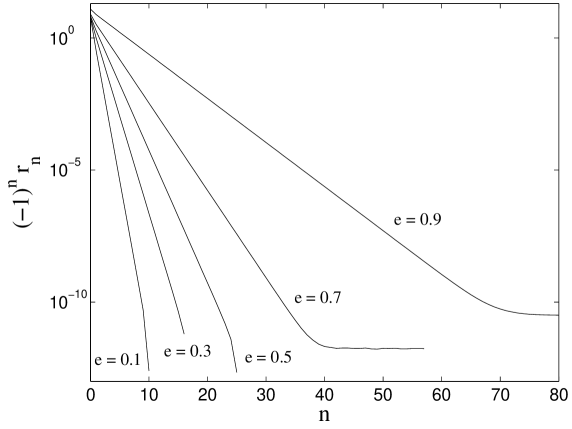
Figure 1: Fourier series coefficients for $r(\lambda)$ in the case of a black hole spin of $a=0.9M$, and geodesics with $p=6$, $\iota=40^{\circ}$. The analogous series for $\theta(\lambda)$, $\phi(\lambda)$, and $t(\lambda)$ converge similarly. The two curves which level out ($e=0.7$ and $e=0.9$) appear to have exhausted the precision capabilities of the numerical method used to produce this plot.

Even for orbits with large eccentricity or inclination, one need only compute a small number of coefficients in the Fourier series in order to evaluate the orbit with great accuracy at arbitrary times. Second, and somewhat surprisingly, it turns out that by exploiting these decompositions, one can show that in the frequency domain associated with coordinate time $t$, most functions of these orbits have a discrete spectrum made up of frequencies [7]

$$f_{mkn}=mf_{\phi}+kf_{\theta}+nf_{r}\;.$$ (2.4)

Here $m$, $k$, and $n$ are integers, while $f_{r}$, $f_{\theta}$, and $f_{\phi}$ are fixed frequencies determined by the boundaries of the orbital torus. For example, if a test particle moves on a fixed geodesic, a distant observer will find that the resulting gravitational waves oscillate only at frequencies $f_{mkn}$.

In the presence of radiation, returning the “I” to EMRI, waveforms observed by distant observers would have a sliding-comb type of frequency-spectrum, a discrete spectrum which over time slides around on the frequency axis. Since these waveforms will likely be weak compared to detector noise, models for the evolution of these spectra will be needed in order to enable some form of matched filtering. The remainder of this article will review EMRI-related work which falls into one of two categories: (i) the calculation of waveforms, and (ii) the development of data analysis algorithms. Since my own research falls into the first category, I will spend more time on the discussion of waveform calculations than on data analysis development. Of course, my bias should not be taken as an indicator of relative importance.

3 Waveforms

Efforts to compute EMRI waveforms can roughly be grouped into three categories: (i) Capra waveforms, (ii) Teukolsky waveforms, and (iii) kludge waveforms. I define the categories as follows (these definitions are described in the following subsections): If a waveform calculation is based on solving the MiSaTaQuWa equations [10, 11], or some higher order version of them, the result is a Capra waveform. If a waveform calculation is based on solving the Teukolsky equation [22, 23, 24], the result is a Teukolsky waveform. If a waveform calculation is based on a variety of formalisms, some of which may even make conflicting assumptions, the result is a kludge waveform. I have listed these categories roughly in order of increasing availability and decreasing accuracy. However, the ultimate categorization factor will be taken to be the method of calculation rather than either its accuracy or availability. I now describe these waveforms, and the status of efforts to compute them

3.1 Capra waveforms

The name Capra comes from the Hollywood film director Frank Capra (1897-1991) whose ranch (which now belongs to Caltech) served as the location for the first of a now-annual series of “Capra meetings”. The ultimate goal of these meetings is to compute a class of waveforms that incorporates the leading-order (in $\mu/M$) effects of both the radiative and conservative parts of the gravitational self-force. The self-force acts on the test mass and is induced by that same object’s perturbation of the background spacetime (it is a force in the sense that, instead of interpreting the motion of the test mass as a geodesic of some perturbed version of the background spacetime, it can be interpreted as being forced to deviate from geodesics of the background.). The radiative part of the self-force produces radiation at the black hole’s horizon and at large radial distances. The conservative part does not produce such radiation, but nonetheless influences the world line of the small object, and the corresponding waveform [12]. Perhaps the crown jewels of efforts toward Capra waveforms are the equations of motion for a test particle under the influence of the first-order parts of the self-force in an arbitrary background spacetime. These are the so-called MiSaTaQuWa equations [10, 11]. I categorize any waveform as a Capra waveform if its calculation was based on solving the MiSaTaQuWa equations, or some higher order version of them. Capra waveforms can be thought of as “holy grail waveforms”. In terms of potential accuracy, they are the most ambitious. They are the only waveforms capable of being computed to an accuracy of order $(\mu/M)^{2}$. Realizing this potential will require computing all of the first-order parts of the self-force, and at least some of its second-order parts [13, 15].

The holy grail characterization of Capra waveforms applies both to their accuracy and availability. To date, no calculation of Capra waveforms exists (with the exception of analog problems for scalar or electromagnetic fields [12]). Perhaps the most advanced effort toward Capra waveforms presented at the 2005 Capra meeting [16] is the work by Barack and Lousto [17]. They developed a numeric code that can compute a waveform for a test mass on an arbitrary worldline in a Schwarzschild background. The code evolves the metric perturbation in the Lorenz gauge, so that the input worldline can be given by the solution of the mode-sum representation of the MiSaTaQuWa equations [18, 19, 20] (known only in the Lorenz gauge, but for any orbit in either Schwarzschild or Kerr backgrounds). Instead of such a worldline, a circular Schwarzschild geodesic is used in Ref. [17]. They successfully compared the power radiated to infinity with results from calculations based on Teukolsky waveforms (discussed below). Incorporating the solution of the mode-sum representation of the MiSaTaQuWa equations into the code from Ref. [17] would produce the first of any subcategory of Capra waveforms.

While progress toward Capra waveforms is steady, much work remains. Second-order versions of the MiSaTaQuWa equations and their solutions must be derived. Then, codes similar to the one used in Ref. [17] must be developed before the full potential of Capra waveforms will be realized. More details on this subject can be found in Poisson’s short manifesto [21] or in his comprehensive treatise [2].

3.2 Teukolsky waveforms

In 1972, Teukolsky derived a powerful equation for describing first-order radiative perturbations of black holes [22, 23, 24]. It applies to cases where the hole is perturbed by a scalar, neutrino, electromagnetic, or gravitational field. Although his is a partial differential equation, Teukolsky showed that it can be separated into a system of ordinary differential equations (ODEs). Solving the Teukolsky equation numerically is therefore far simpler than traditional numerical relativity [29]. I categorize any waveform as a Teukolsky waveform if its calculation was based on solving the Teukolsky equation. Since solutions of the Teukolsky equation describe only radiative first-order (in $\mu/M$ for the case of EMRIs) effects, Teukolsky waveforms have less potential accuracy than Capra waveforms which, at least in principle, can also describe second-order and conservative effects.

The calculation of Teukolsky waveforms has been something of an industry since the early 1990’s (see table I of Ref. [8]). These calculations exploit the condition that the test mass moves in an orbit-like fashion, so that Eq. (1.2) holds. The source term in the Teukolsky equation is taken to be a point-particle on a bound geodesic of the background spacetime. Since the equation’s solution contains all the radiative information, it describes the waveform produced by the particle’s motion, and also the effect of that radiation on the orbit. By iteration, the orbit evolves from a geodesic to an inspiral while the waveform evolves from only a “snapshot” of what an observer would see over a short time, to the entire EMRI waveform. This strategy has only recently been applied to generic black hole orbits with both eccentricity $e\neq 0$ and inclination $\iota\neq 0^{\circ},180^{\circ}$. The radiation snapshots produced by these orbits have been computed numerically [30, 8, 9], but the iteration needed to produce the full EMRI waveform is still under development. I now sketch a few of the details of these new developments.

As is described in Sec. 1, many functions of generic black hole orbits have a discrete frequency-spectrum at frequencies $f_{mkn}$, given by Eq. (2.4). The radiation produced by a test mass moving on that orbit is one such function. A distant observer would see that radiation as the following waveform

$$h_{+}-ih_{\times}=-\frac{2}{r}\sum_{l=2}^{\infty}\sum_{m=-l}^{l}\sum_{k=-\infty}^{\infty}\sum_{n=-\infty}^{\infty}\frac{Z^{\rm{H}}_{lmkn}}{\omega_{mkn}^{2}}S_{lmkn}(\theta)e^{-i\omega_{mkn}(t-r)+im\phi+i\chi_{lmkn}}\;.$$ (3.1)

Here $h_{+}$ and $h_{\times}$ are the two independent components of the metric perturbation, $\omega_{mkn}=2\pi f_{mkn}$, and both the coefficients $Z^{\rm{H}}_{lmkn}$ and the functions $S_{lmkn}(\theta)$ are found by solving the ODEs that separate out from the Teukolsky equation . The phase constants $\chi_{lmkn}$ in Eq. (3.1) are determined by the initial position of the test mass , and can be set to zero when considering a fixed orbit. Similar expressions for the radiative changes in the orbiting particle’s energy $E$, axial angular momentum $L$, and Carter constant $Q$ have been derived [30, 28, 26, 27]. For example, the average change in the orbital energy is given by

$$\left<\frac{dE}{dt}\right>=\sum_{l=2}^{\infty}\sum_{m=-l}^{l}\sum_{k=-\infty}^{\infty}\sum_{n=-\infty}^{\infty}\frac{1}{4\pi\omega_{mkn}^{2}}\left(\left|Z^{\rm{H}}_{lmkn}\right|^{2}+\alpha_{lmkn}\left|Z^{\infty}_{lmkn}\right|^{2}\right)\;,$$ (3.2)

where $\alpha_{lmkn}$ are simple constants that are analytically known [8], and $Z^{\infty}_{lmkn}$ are similar to $Z^{\rm{H}}_{lmkn}$. The geometry of the orbit dictates which terms are significant in Eqs. (3.1) and (3.2). If the orbit is both circular and equatorial, all of the terms with $k\neq 0$ and $n\neq 0$ vanish. Similarly, for orbits with eccentricity above about $0.3$ and inclination below about $60^{\circ}$, one captures better than half of the radiation by keeping only the terms with $k=0$ [8].

Summing over only one of the terms in the parentheses of Eq. (3.2) gives either the power radiated at large radial distances, or into the horizon. One normally would arrive at this formula by first deriving each sum independently, and then enforcing global energy conservation [31]. This derivation has a major drawback. It is not generalizable to the evolution of the Carter constant. Alternatively, one can derive the same result as follows. First, solve the Teukolsky equation (this gives the radiation field, or equivalently $Z^{\infty}_{lmkn}$ and $Z^{\rm{H}}_{lmkn}$). Second, express the radiative self-force in terms of the radiation field. Third, express the average rate of change in the orbital constant of interest in terms of the radiative self-force. Galt’sov showed that, under general circumstances, this gives the traditional result [31] when applied to both energy and angular momentum [32]. At the time however, the validity of using only the radiative self-force was not known. Mino has since proved this to be valid [6], and the method has now been used to describe the evolution of the Carter constant in terms of the same quantities used for energy and angular momentum (namely $Z^{\infty}_{lmkn}$ and $Z^{\rm{H}}_{lmkn}$) [30, 28, 26, 27]. Although the final equation for $\left<dQ/dt\right>$ in Refs. [30, 28] appear different from the more concise result in Refs. [26, 27], their equivalence has since been shown [33].

It has recently been demonstrated that, for an analogous case of an electric charge moving on a Newtonian orbit, one must account for the evolution of $\chi_{lmkn}$ in Eq. (3.1) in order to compute the full EMRI waveform to leading order in the charge to mass ratio [12]. Also, for the case considered in Ref. [12], the evolution of $\chi_{lmkn}$ was completely determined by the conservative self-force alone. Solutions to the Teukolsky equation contain only radiative information, so if this result carries over to the strong field regime relevant to EMRI observations, it will severely decrease the usefulness of both Teukolsky waveforms and kludge waveforms (described below). It should be emphasized however that the analysis in Ref. [12] applies in the limit where gravity is Newtonian, and that some of their findings are expected to be atypical of the strong field regime (see the last several paragraphs of Sec. V in Ref. [12]). Even if their results apply partially to the strong field, so that in the strong field the evolution of $\chi_{lmkn}$ is observationally significant, but can be well approximated from the radiative self-force alone, the equations governing such an evolution have yet to be derived. Though such equations should in principle be obtainable from the analysis in Appendix C of Ref. [14], the resolution to this problem remains a subject of current research [15].

There is also a history of efforts to solve the Teukolsky equation without fully exploiting its separability—only the $\phi$-coordinate is separated such that the codes must solve a “$2+1$” dimensional partial differential equation. These “time-domain” calculations have yet to match the precision of their “frequency-domain” alternatives. In the most generic time-domain calculation to date (equatorial or circular Kerr orbits [34]) total fluxes of energy and angular momentum agreed with frequency-domain codes to within about 25%, whereas independent frequency-domain codes often agree to as many as six digits [8]. However, recent improvements in time-domain methods, including the use of an adaptive mesh, are promising. Such codes have so far been applied to Schwarzschild [35]. There agreement with frequency-domain codes improved by about a factor of ten over the previous generation of time-domain codes, agreeing to within about 0.01%. See Ref. [35] for a discussion of the possible advantages of time-domain methods.

3.3 Kludge waveforms

I categorize any waveform as a kludge waveform if its calculation was based on a collection of different formalisms, some of which may even make conflicting assumptions (i.e. solving the flat-space quadrupole formula for a particle on a relativistic black hole orbit). Kludge waveforms are in generally less accurate than Capra or Teukolsky waveforms. However as more rigorous waveforms have become available, kludge waveforms have made good on their promise of capturing the dominant features of the more realistic waveforms [36]. Kluge waveforms are readily available, and can be computed very quickly. This makes them the tool of choice when scoping out candidate data analysis techniques (discussed in the next section). Their flexible design allows one to experiment freely, although admittedly crudely, by adding and removing proposed physical effects which would be unimaginably difficult to incorporate into Capra or Teukolsky waveform calculations. For example, kludge waveforms are already available for speculative non-Kerr background space-times that may be used in straw-man/null-experiment tests of general relativity [37, 38]. In principle, kludge waveforms can also include effects due to the conservative self-force [36, 43]. Kludge waveforms may be lacking in rigor and perfection, but they overflow with availability and adaptability.

The majority of kludge waveform calculations are numerical. I now describe the analytical exceptions. As early as 1963, Peters and Mathews derived waveforms for eccentric Newtonian orbits using the flat space quadrupole formula [39]. Barack and Cutler [40] stiched together sequences of those waveforms by using post-Newtonian formulas to evolve the constants of orbital motion. This enabled them to account for relativistic effects including those due to the black hole’s spin, precession of the perihelion, and Lense-Thirring precession. The post-Newtonian formalism is generally invalid for EMRIs, since the test mass moves at nearly light-speed. However, their waveforms were useful for making rough estimates of how well LISA could measure an EMRIs parameters [40]. These analytic kludge waveforms will also likely be used in the future for a LISA Mock Data Challenge, a project that will use simulated LISA data to test proposed data analysis techniques for a variety of sources (initial results will be announced at the 2006 GWDAW meeting). Another analytic effort, originally motivated as a tool for exploring convergence of post-Newtonian series and for improving waveforms for neutron star binaries, derives the post-Newtonian expansion to solutions of the Teukolsky equation [3]. This hybrid technique assumes both a small mass ratio and slow motion. The most recent contribution to this effort applies to Kerr orbits which are both slightly inclined and slightly eccentric [27], and it is anticipated that the same calculation will soon be complete for arbitrary inclination [44]. Table 1 shows that the hybrid calculation of radiative fluxes of energy and angular momentum [27] compared well with pure Teukolsky calculations [8].

$e$	$\iota$	disagreement in radiative power	disagreement in radiative torque
0.03	$1.7^{\circ}$	$0.019~{}20\%$	$0.013~{}23\%$
0.03	$3.4^{\circ}$	$0.019~{}22\%$	$0.013~{}22\%$
0.03	$5.2^{\circ}$	$0.019~{}26\%$	$0.013~{}19\%$
0.06	$1.7^{\circ}$	$0.163~{}7~{}\%$	$0.075~{}23\%$
0.06	$3.4^{\circ}$	$0.163~{}8~{}\%$	$0.075~{}14\%$
0.06	$5.2^{\circ}$	$0.163~{}8~{}\%$	$0.074~{}97\%$
0.09	$1.7^{\circ}$	$0.734~{}9~{}\%$	$0.319~{}8~{}\%$
0.09	$3.4^{\circ}$	$0.734~{}9~{}\%$	$0.319~{}4~{}\%$
0.09	$5.2^{\circ}$	$0.734~{}9~{}\%$	$0.318~{}7~{}\%$

Table 1: Comparison of numerical solutions to the Teukolsky equation [8, 9] with analytical post-Newtonian expansions of those solutions [27]. Here the black hole has spin $a=0.9M$, and the orbits have semilatus rectum $p=100$. The dependence of the disagreement on the orbital parameters is the expected result of the hybrid calculation’s use of a truncated Taylor expansion in both eccentricity $e$ and inclination $\iota$.

The following is a rough outline of the procedure used to compute kluge waveforms numericaly: First, evolve the orbital constants by integrating equations of the form

$$\frac{d\mathcal{E}}{dt}=Y(\mathcal{E},a,M,\mu)\;,$$ (3.3)

where $\mathcal{E}=(E,L,Q)$, or $\mathcal{E}=(e,p,\iota)$, to obtain $\mathcal{E}(t)$. Since $(E,L,Q)$ can be translated exactly to $(e,p,\iota)$, and vice versa, the choice here is somewhat arbitrary. These equations might be, say, analytical post-Newtonian approximations, or some numerical formula gleamed from a fit to numerical data from solving the Teukolsky equation. Second, using these solutions, determine the inspiraling world line ${\bf x}(t)$ by integrating a system of geodesic equations of the form (e.g. Carter’s equations [41] if the background is Kerr)

$$\frac{d{\bf x}}{dt}={\bf V}[\mathcal{E}(t),a,M,\mu]\;.$$ (3.4)

Third, obtain the waveform by solving an equation of the form

$$h_{ij}({\bf x}_{\rm{field}},t)=W_{ij}({\bf x}_{\rm{field}},{\bf x}[t])\;,$$ (3.5)

where here the subscript “field” denotes the position of the observer. Examples of such an equation might be the flat space quadruple, or quadruple plus octupole formulas.

This numerical kludge procedure has been followed by several groups using a variety of different approximate formulas at each step [42, 36, 43]. The first step of this procedure, integrating the equation that evolves orbital constants (3.3), has been executed by Gair and Glampedakis for the case of generic black hole orbits [36]. In a separate calculation, for a fixed generic black hole orbit that does not inspiral, Babak et al [43] obtained snapshots of generic kludge waveforms by completing steps two and three [solving Eqs. (3.4) and (3.5) with $\mathcal{E}$ held fixed]. They found remarkable agreement when comparing with Teukolsky waveforms (see Fig. 2).

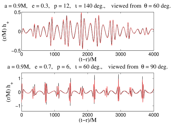
Figure 2: Comparison of Teukolsky [8, 9] (black) and numeric kludge [43] (red, or light gray) waveform snapshots for two different generic black hole orbits. The parameters of the black hole and the orbits are shown in the titles above the plots. This level of agreement continues for essentially all time. The short time range shown here was used so that the reader can get a feel for the overlap by eye. The overlap estimates are 99% for the top panel (over a time of 20,000 $M$) and 97% for the bottom panel (over a time of 15,000 $M$).

Estimates of the overlap between those kludge waveforms [43] and Teukolsky waveforms [8, 9] were typically around 98%, for $p\gtrsim 6$. This high level of agreement suggests that kludge waveforms may ultimately be used directly in EMRI detection algorithms, as opposed to being used only when exploring data analysis options (that is, data analysis analysis). These two works [36, 43] will likely soon be merged in order to produce generic kludge waveforms which represent the entire inspiral.

Another recent set of interesting kludge waveforms are those produced by test particles moving on equatorial orbits of a “quasi-Kerr” background spacetime (a spacetime which is identical to Kerr, but which has a perturbed quadrupole moment, see Ref. [38] for further details). Those authors found that, by varying the orbital parameters, one could generally find a background-orbit pair (Kerr, geodesic orbit) which resulted in waveforms with a high overlap ($>90\%$) compared to some pair (quasi-Kerr, geodesic orbit). If this holds true in general, the common wisdom that the waveform is a unique signature of the black hole will be cast into doubt. It seems likely that this “confusion problem” won’t persist when one includes the effects of radiation and generic orbits. Radiation may shift the orbit-pairs away from the overlaping regime. Also, the high overlap required common orbital frequencies, but it is not yet clear that generic quasi-Kerr orbits have orbital frequencies (as opposed to continuous spectra). Nevertheless, the question of whether or not the confusion problem is general remains open.

4 Data analysis

Even if all three classes of waveforms (Capra, Teukolsky, and kludge) were readily available, the problem of extracting EMRI waveforms from data would remain non-trivial. In this section I briefly describe the status of efforts to develop EMRI data analysis algorithms for LISA. As promised, this section will be less detailed than the previous section on waveform calculations. A more thorough review of these issues can be found in Ref. [45].

Gair et al [45] estimate that a “brute force” matched filter search algorithm (akin to LIGO searches for neutron star binaries [46]) that uses year-long template waveforms to find EMRIs would require on the order of $10^{40}$ templates, rendering it computationally impractical. Their favored practical alternative is a heirarchical search which begins with short duration templates (lasting a few weeks) of modest accuracy. It should be emphasized that the full year or so worth of data is used at this stage—it is only the waveforms which are short. One still needs a scheme for jumping from one short waveform to the next, but that scheme does not demand modeling the phase evolution for times longer than a few weeks. This segment of the search can be thought of as the “detection stage” in which EMRI candidates are identified, and relatively modest estimates of their parameters are made. The search would then proceed toward a “measurement stage” which focuses in on narrow regions of parameter space using increasingly accurate and longer-lasting templates, and which realizes LISA’s full sensitivity (e.g. measuring $\mu$, $M$, and $a$ with fractional accuracy $\sim 10^{-4}$ [40]). They estimate that such a scheme would yield anywhere from tens to thousands of EMRI observations over LISA’s lifetime .

In the hierarchical search envisioned in Ref. [45], Teukolsky waveforms (or perhaps even kludge waveforms) lasting up to a few weeks will likely suffice as templates for the initial detection stage, whereas Capra waveforms lasting up to a few years will be needed for the final measurement stage. Let’s focus now on the detection stage. The number of waveform snapshots (waveforms produced by a single fixed geodesic) needed to produce sufficiently accurate detection waveforms is currently unknown. For example, it is possible that snapshots alone might suffice as detection templates. If so, then the tools for EMRI detection are available already [8]. The following simple scaling argument would seem to suggest that snapshots cannot be used as detection templates. Expand the $\phi$ coordinate of the test mass’ world line (a quantity interchangeable with the phase of the waveform for purposes of this rough argument) as follows:

$$\phi(t)=\phi_{0}+{\dot{\phi}_{0}}t+\frac{1}{2}{\ddot{\phi}}_{0}t^{2}+\cdots\;.$$ (4.1)

Here $\phi_{0}$, ${\dot{\phi}}_{0}$, and ${\ddot{\phi}}_{0}$ are constants. The first two terms would be exact for a circular-equatorial geodesic, while the third term represents the effect of radiation. A waveform constructed from the geodesic terms alone would produce a phase error of order unity after a time $T_{\rm{snap}}$, where ${\ddot{\phi}}_{0}T_{\rm{snap}}^{2}\sim 1$. By dimensional analysis, one would expect ${\dot{\phi}_{0}}M\sim 1$ and ${\ddot{\phi}_{0}}M^{2}\sim\mu/M$. This suggests that the waveform snapshot would be valid for times shorter than

$$T_{\rm{snap}}\sim M\sqrt{M/\mu}\;.$$ (4.2)

This equation predicts that, for EMRIs that could be observed with LISA, a single snapshot would accurately represent the waveform for times ranging from a few seconds to a day or so—hardly the few weeks demanded [45] of detection templates. However, this is only a scaling argument, and it neglects potentially significant coefficients which must diverge as the Newtonian limit is approached. Recently, Glampedakis and Babak estimated values for $T_{\rm{snap}}$ by comparing snapshots of Teukolsky waveforms to kludge inspiral waveforms in the case of eccentric-equatorial orbits [38]. They found, even for orbits relatively close to the horizon, that Eq. 4.2 underestimates $T_{\rm{snap}}$ by a significant factor $T_{\rm{snap}}/(M\sqrt{M/\mu})\sim 100$ (see Fig. 3).

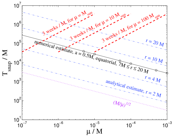
Figure 3: Snapshot timescale $T_{\rm{snap}}/M$ versus mass ratio $\mu/M$ for a black hole spin of $a=0.5M$, and a geodesic with $e=0.5$, $p=10$, and $\iota=0^{\circ}$. The (black) solid-line and circles are numerical estimates reported by Glampedakis and Babak [38]. The (blue) dashdot lines are the analytical estimate (1.10) evaluated at the indicated orbital radii, $r/M=$ 2, 4, 10, and 20. The (magenta) dotted line is the estimate from the scaling argument $T_{\rm{snap}}=M\sqrt{M/\mu}$. If waveform snapshots are to be sufficient for detection, they must have $T_{\rm{snap}}>$ 3 weeks. This boundary is shown as (red) dashed lines for a few different test masses $\mu$.

An alternative analytical estimate (1.10), shown in Fig. 3 and derived in the appendix below, gives similar results. These results suggest that existing waveform snapshots will suffice for detection, at least for some subset of EMRIs that could be observed by LISA.

Lastly, I want to address a topic which is relevant to EMRIs, but which is also of general interest for LISA data analysis as a whole. One of the key differences between LISA and LIGO-like detectors is that LISA is anticipated to find an over abundance of sources. This very attractive feature also poses a potential problem in that waveforms from many different sources will overlap each other, complicating the task of cleanly identifying any one of the sources. For example, the waveforms produced by galactic compact binaries (GCBs, e.g. a pair of white dwarfs) are nearly monochromatic, so that a collection of thousands of these waveforms resembles a Fourier basis complete enough to fit essentially any smooth function in their frequency band. Therefore, an attempt to first subtract thousands of galactic binary waveforms from LISA data before searching for other signals is likely to (i) produce erroneous population statistics for the GCBs and (ii) doom further searches by washing away any remaining signals. In order to avoid this problem, LISA data analysis algorithms will simultaneously search for a variety of different sources. Algorithms that detect single waveforms in isolation are an essential ingredient to this process, however the isolated techniques will ultimately be merged into one “global fit” algorithm.

When it comes to LISA’s general need for global fit algorithms, EMRIs are no exception to the rule. Their lower frequencies will likely be hidden by a background of unresolved GCBs, and their observable band is expected to overlap with resolvable GCBs and mergers of massive black holes [47]. Recent advances toward global fit data analysis techniques can be found in Refs. [48, 49]. Though these works do not deal with EMRIs, similar work must eventually do so, and these are good indicators of general progress toward global fit analysis for LISA. In Ref. [48], a “reversible jump Markov chain Monte Carlo” technique is used to simulate the detection and measurement of 100 monochromatic signals. In Ref. [49], similar techniques are implemented for up to 10 GCBs. See also the two contributions by J. Crowder and by E. D. M. Wickham to this meeting (GWDAW 10). These works differ more in their numerical methods than in their theoretical foundations. They each represent implementations of Bayesian Inference [50].

5 Provocation

The conference organizers asked for a review that would provoke discussion. In case I have failed to provoke anyone so far, this list of questions (and my guessed answers ) might: Could EMRI detections be made using only the existing waveform snapshots as detection templates? (This would work for some EMRIs with $\mu/M\lesssim 10^{-5}$.) Can kludge waveforms be used as detection templates? (Probably, but other waveforms will be needed in order to determine which kludges suffice.) Is the conservative self-force needed for detection? (No, but it will be needed for detailed EMRI measurements.) Are EMRI waveforms really unique signatures of the background spacetime, or is there instead a Kerr versus non-Kerr confusion problem? (Including the effects of radiation and generic orbits will show that there is no confusion problem.) What are the prospects for global fit data analysis techniques? (It is difficult to speculate quantitatively on the prospects for this field. However, this type of analysis is a hot topic in many fields that are otherwise unrelated to gravitational wave detection [50]. Due to the rapid growth in the field, as evidenced by the regular additions to lists of relevant papers [51], it seems wise to develop as many independent global fit methods as possible.) Should we look for IMRIs with ground-based detectors? (Yes, little is know about the sources, and searches can be done immediately.) Detailed analyses of any of these questions would likely make a significant contribution toward eventual EMRI observations.

Appendix A Analytic estimate of $T_{\rm{snap}}$

I thank Éanna Flanagan for permission to include this paraphrasing of his analytical estimate for the time $T_{\rm{snap}}$ over which waveform snapshots are valid.

Suppose that an EMRI’s true orbital phase $\phi_{\rm{true}}(t)$ can be approximated as a quadratic in time, as in Eq. (4.1), while the orbital phase used to compute a waveform snapshot template $\phi_{\rm{temp}}(t)$ is only linear in time, as would be the case if the snapshot was produced by a test mass on a circular orbit. Take the true and approximate waveforms to have the form $h=A\cos[2\phi(t)]$, where $A$ is constant, and $\phi(t)$ is the corresponding orbital phase

$$h_{\rm{true}} = A\cos(2\phi_{\rm{true}})=A\cos(2\phi_{0}+2{\dot{\phi}_{0}}t+{\ddot{\phi}}_{0}t^{2})~{},$$ (1.1)

$$h_{\rm{temp}} = A\cos(2\phi_{\rm{temp}})=A\cos(2\phi_{0}+2{\dot{\phi}_{0}}t)~{}.$$ (1.2)

Also assume for simplicity that the average overlap integral over a time $T$ is just a time integral, from $-T/2$ to $T/2$, of the product of two waveforms, divided by $T$. The average overlap of the waveforms $h_{\rm{true}}$ and $h_{\rm{temp}}$ is then

$$V_{\rm{avg}}(T)=\frac{A^{2}}{2T}\int_{-T/2}^{T/2}dt~{}\cos(2\phi_{\rm{true}}+2\phi_{\rm{temp}})+\frac{A^{2}}{2T}\int_{-T/2}^{T/2}dt~{}\cos(2\phi_{\rm{true}}-2\phi_{\rm{temp}})~{}.$$ (1.3)

The first term in this expression vanishes rapidly, and is presumably unobservable. The second term dominates since it approaches zero very slowly (typically on time scale that is many orders of magnitude longer than the time needed for the first term to vanish). The normalized overlap (in the sense that it goes to unity for a pair of identical waveforms) of these two waveforms is then given by

$$V_{\rm{norm}}(T)=\frac{1}{T}\int_{-T/2}^{T/2}dt~{}\cos(2\phi_{\rm{true}}-2\phi_{\rm{temp}})~{}.$$ (1.4)

Substitution of the phases read off from the waveforms (1.1) and (1.2) gives

$$V_{\rm{norm}}(T)=\frac{1}{T}\int_{-T/2}^{T/2}dt~{}\cos({\ddot{\phi}}_{0}t^{2})=\frac{C[x(T)]}{x(T)}~{},$$ (1.5)

where

$$C(x)=\int_{0}^{x}dt~{}\cos(\pi t^{2}/2)~{},$$ (1.6)

is the Fresnel cosine integral, and where

$$x(T)=T\sqrt{\frac{{\ddot{\phi}}_{0}}{2\pi}}~{}.$$ (1.7)

As in Ref. [38], define the time at which the approximate waveform is invalid $T_{\rm{snap}}$ to be the time at which the overlap $V_{\rm{norm}}$ drops to 95%. Solving $C(x)/x=0.95$ gives $x=x_{0}=0.67\approx 2/3$, which gives

$$T_{\rm{snap}}^{2}=\frac{8\pi}{9}{\ddot{\phi}_{0}}^{-1}~{}.$$ (1.8)

Now use the Newtonian formula (from Sec. III of Ref. [52] with $\Omega={\dot{\phi}_{0}}$ and ${\dot{\Omega}}={\ddot{\phi}_{0}}$),

$${\ddot{\phi}}_{0}=\frac{96}{5}\mu M^{2/3}{\dot{\phi}}_{0}^{11/3}~{},$$ (1.9)

and approximate the orbital frequency $\dot{\phi}_{0}$ with Kepler’s law $r/M=(M{\dot{\phi}_{0}})^{-2/3}$, to find

$$T_{\rm{snap}}=\left[\sqrt{\frac{5\pi}{108}}\left(\frac{r}{M}\right)^{11/4}\right]M\sqrt{\frac{M}{\mu}}~{}.$$ (1.10)

As expected, this improved estimate diverges in the Newtonian limit $r/M\to\infty$. Over the range of innermost stable circular orbits of rotating black holes $1\leq r/M\leq 9$, it differs from the result of the simple scaling argument by a factor ranging roughly from $38\%$ to $160$.

References

References

- [1] K. Glampedakis, Extreme mass ratio inspirals: LISA’s unique probe of black hole gravity, Class. Quant. Grav., 22, S605–S659 (2005).
- [2] E. Poisson, The Motion of Point Particles in Curved Spacetime, Living Rev. Relativity 7, 6 (2004), http://www.livingreviews.org/lrr-2004-6 .
- [3] M. Sasaki and H. Tagoshi, Analytic Black Hole Perturbation Approach to Gravitational Radiation, Living Rev. Relativity 6, 6 (2003), http://www.livingreviews.org/lrr-2003-6/ .
- [4] S. A. Hughes, Evolution of circular, nonequatorial orbits of Kerr black holes due to gravitational-wave emission, Phys. Rev. D 61, 084004 (2000); Phys. Rev. D 63, 049902(E) (2001); Phys. Rev. D 65, 069902(E) (2002); Phys. Rev. D 67, 089901(E) (2003).
- [5] D. Brown et al, in preperation.
- [6] Y. Mino, Perturbative approach to an orbital evolution around a supermassive black hole, Phys. Rev. D 67, 084027 (2003).
- [7] S. Drasco and S. A. Hughes, Rotating black hole orbit functionals in the frequency domain, Phys. Rev. D 69, 044015 (2004).
- [8] S. Drasco and S. A. Hughes, Gravitational wave snapshots of generic extreme mass ratio inspirals, Phys. Rev. D 73 (2006).
- [9] Waveforms and flux data described in Ref. [8], and for thousands of other generic orbital configurations, have been made public at http://gmunu.mit.edu/sdrasco/snapshots/ . The supercomputers used in that investigation were provided by funding from JPL Institutional Computing and Information Services and the NASA Directorates of Aeronautics Research, Science, Exploration Systems, and Space Operations.
- [10] Y. Mino, M. Sasaki, and T. Tanaka, Gravitational radiation reaction to a particle motion, Phys. Rev. D 55, 3457 (1997).
- [11] T. C. Quinn and R. M. Wald, Axiomatic approach to electromagnetic and gravitational radiation reaction of particles in curved spacetime, Phys. Rev. D 56, 3381 (1997).
- [12] A. Pound, E. Poisson, and B. G. Nickel, Limitations of the adiabatic approximation to the gravitational self-force, Phys. Rev. D 72, 124001 (2005).
- [13] E. Rosenthal, Construction of the second-order gravitational perturbations produced by a compact object, Phys. Rev. D 73, 044034 (2006).
- [14] Y. Mino, Self-Force in the Radiation Reaction Formula, Prog. Theor. Phys. 113 , 733 (2005).
- [15] T. Hinderer and É. É. Flanagan, in preparation.
- [16] The presentations from this meeting can be found online at http://www.sstd.rl.ac.uk/capra .
- [17] L. Barack and C. O. Lousto, Perturbations of Schwarzschild black holes in the Lorenz gauge: Formulation and numerical implementation, Phys. Rev. D 72, 104026 (2005).
- [18] L. Barack and A. Ori, Mode sum regularization approach for the self-force in black hole spacetime, Phys. Rev. D 61, 061502 (2000).
- [19] L. Barack, Y. Mino, H. Nakano, A. Ori, and M Sasaki, Calculating the Gravitational Self-Force in Schwarzschild Spacetime, Phys. Rev. Lett. 88, 091101 (2002).
- [20] L. Barack and A. Ori, Gravitational Self-Force on a Particle Orbiting a Kerr Black Hole, Phys. Rev. Lett. 90, 111101 (2003).
- [21] E. Poisson, The gravitational self-force, gr-qc/0410127.
- [22] S. A. Teukolsky, Rotating Black Holes: Separable Wave Equations for Gravitational and Electromagnetic Perturbations, Phys. Rev. Lett. 29, 1114 (1972).
- [23] S. A. Teukolsky, Perturbations of a rotating black hole. I. fundamental equations for gravitational, electromagnetic, and neutrino-field perturbations, Astrophys. J. 185, 635 (1973).
- [24] M. P. Ryan Jr., Teukolsky equation and Penrose wave equation, Phys. Rev. D 10, 1736 (1974). This reference gives an interesting alternative derivation of the Teukolsky equation, “from a second-order wave equation for the Riemann tensor.”
- [25] S. Chandrasekhar, The Mathematical Theory of Black Holes (Oxford University Press, New York, 1983).
- [26] N. Sago, T. Tanaka, W. Hikida, and H. Nakano, Adiabatic radiation reaction to the orbits in Kerr Spacetime, Prog. Theor. Phys. 114 , 509 (2005).
- [27] N. Sago, T. Tanaka, W. Hikida, H. Nakano, K. Ganz, The adiabatic evolution of orbital parameters in the Kerr spacetime, Prog. Theor. Phys. 115, 873 (2006).
- [28] S. Drasco, É. É. Flanagan, and S. A. Hughes, Computing inspirals in Kerr in the adiabatic regime. I. The scalar case, Class. Quantum Grav. 22, S801 (2005).
- [29] T. W. Baumgarte and S. L. Shapiro, Numerical relativity and compact binaries, Phys. Rep. 376, 41 (2003).
- [30] S. A. Hughes, S. Drasco, É. É. Flanagan, and J. Franklin, Gravitational radiation reaction and inspiral waveforms in the adiabatic limit, Phys. Rev. Lett. 94, 221101 (2005).
- [31] S. A. Teukolsky and W. H. Press, Perturbations of Rotating Black Hole. III. Interaction of the Hole with Gravitational and Electromagnetic Radiation, Astrophys. J. 193, 443 (1974).
- [32] D.V. Gal’tsov. Radiation reaction in the Kerr gravitational field, J. Phys A: Math. Gen. 15, 3737 (1982).
- [33] N. Sago and S. Drasco, in preparation.
- [34] G. Khanna, Teukolsky evolution of particle orbits around Kerr black holes in the time domain: Elliptic and inclined orbits, Phys. Rev. D 69, 024016 (2004).
- [35] C. F. Sopuerta and P. Laguna, A Finite Element Computation of the Gravitational Radiation emitted by a Point-like object orbiting a Non-rotating Black Hole Phys. Rev. D 73, 044028 (2006).
- [36] J. R. Gair and K. Glampedakis, Improved approximate inspirals of test-bodies into Kerr black holes, Phys. Rev. D 73, 064037 (2006).
- [37] N. A. Collins and S. A. Hughes, Towards a formalism for mapping the spacetimes of massive compact objects: Bumpy black holes and their orbits, Phys. Rev. D 69, 124022 (2004).
- [38] K. Glampedakis and S. Babak, Mapping spacetimes with LISA: inspiral of a test-body in a ‘quasi-Kerr’ field, Class. Quant. Grav. 23, 4167 (2006).
- [39] Gravitational Radiation from Point Masses in a Keplerian Orbit. P. C. Peters and J. Mathews, Phys. Rev. 131, 435 (1963).
- [40] L. Barack and C. Cutler, LISA capture sources: approximate waveforms, signal-to-noise ratios, and parameter estimation accuracy Phys. Rev. D 69, 082005 (2004).
- [41] B. Carter, Global structure of the Kerr family of gravitational fields, Phys. Rev. 174, 1559 (1968).
- [42] K. Glampedakis, S. A. Hughes, and D. Kennefick, Approximating the inspiral of test bodies into Kerr black holes; Phys. Rev. D 66, 064005 (2002).
- [43] S. Babak, H. Fang, J. R. Gair, K. Glampedakis, and S. A. Hughes, “Kludge” gravitational waveforms for a test-body orbiting a Kerr black hole, gr-qc/0607007.
- [44] N. Sago, private communication (2005).
- [45] J. R. Gair et al, Event rate estimates for LISA extreme mass ratio capture sources, Class. Quant. Grav. 21, S1595-S1606(2004).
- [46] LIGO Scientific Collaboration: B. Abbott et al, Search for gravitational waves from galactic and extra–galactic binary neutron stars, Phys. Rev. D 72, 082001(2005).
- [47] E. Berti, LISA observations of massive black hole mergers: event rates and issues in waveform modeling, astro-ph/0602470.
- [48] R. Umstätter, et al, Bayesian modeling of source confusion in LISA data, Phys. Rev. D 72, 022001 (2005).
- [49] N. J. Cornish and J. Crowder, LISA Data Analysis using MCMC methods, Phys. Rev. D 72, 043005 (2005).
- [50] T. J. Loredo, Computational technology for Bayesian inference, in Astronomical Society of the Pacific Conference Series, San Francisco, 1999, edited by R. (Dick) Crutcher and D. Mehringer, vol 172, p. 297.
- [51] See the MCMC preprint service http://www.statslab.cam.ac.uk/mcmc/pages/latest.html .
- [52] L. S. Finn and K. S. Thorne, Gravitational waves from a compact star in a circular, inspiral orbit, in the equatorial plane of a massive, spinning black hole, as observed by LISA, Phys. Rev. D 62, 124021 (2000).