Merger Transitions in Brane–Black-Hole Systems:
Criticality, Scaling, and Self-Similarity

Abstract

We propose a toy model for study merger transitions in a curved spaceime with an arbitrary number of dimensions. This model includes a bulk $N$-dimensional static spherically symmetric black hole and a test $D$-dimensional brane ($D\leq N-1$) interacting with the black hole. The brane is asymptotically flat and allows $O(D-1)$ group of symmetry. Such a brane–black-hole (BBH) system has two different phases. The first one is formed by solutions describing a brane crossing the horizon of the bulk black hole. In this case the internal induced geometry of the brane describes $D$-dimensional black hole. The other phase consists of solutions for branes which do not intersect the horizon and the induced geometry does not have a horizon. We study a critical solution at the threshold of the brane-black-hole formation, and the solutions which are close to it. In particular, we demonstrate, that there exists a striking similarity of the merger transition, during which the phase of the BBH-system is changed, both with the Choptuik critical collapse and with the merger transitions in the higher dimensional caged black-hole–black-string system.

I Introduction

Caged (Kaluza-Klein) black holes, black strings, and possible transitions between them is a subject which has recently attracted a lot of attention (see e.g. reviews HO ; kol1 and references therein). Kol kol demonstrated that during the black-hole–black-string transition the Euclidean topology of the system changers. These transitions were called merger transitions. One of the interesting features of the merger transitions kol is their close relation to the Choptuik critical collapse phenomenon chop . The merger transitions are in many aspects similar to the topology change transitions in the classical and quantum gravity (see e.g. hor and references therein). In particular, one can expect that during both types of transitions the spacetime curvature can infinitely grow. It means that the classical theory of gravity is not sufficient for their description and a more fundamental theory (such as the string theory) is required. In these circumstances, it might be helpful to have a toy model for the merger and topology changing transitions, which is based on the physics which is well understood. In this paper we would like to propose such a toy model.

The model consists of a bulk $N$-dimensional black hole and a test $D$-dimensional brane in it ($D\leq N-1$). We assume that the black hole is spherically symmetric and static. It can be neutral or charged. As we shall see the detailed characteristics of the black hole are not important for our purposes. We assume that the brane is infinitely thin and use the Dirac-Nambu-Goto D ; NG equations for its description. We consider the brane which is static and spherically symmetric, so that its worldsheet has the $O(D-1)$ group of the symmetry. We assume also that the brane reaches the asymptotic infinity where it has the form of the $(D-1)$-plane. One more dimension the brane worldsheet gets because of its time evolution. To keep the brane static one needs to apply a force to it. The detailed mechanism is not important for our consideration, so that we do not discuss it here.

As a result of the gravitational attraction, the brane, which is flat at infinity, is deformed. There are two different types of possible equilibrium configurations. A brane either crosses the black hole horizon, or it lies totally outside the black hole. In the former case the internal metric of the brane, induced by its embedding, describes a geometry of $D$-dimensional black hole. This happens because the timelike at infinity Killing vector of the bulk geometry being restricted to the brane is the Killing vector for the induced geometry. Thus the brane spacetime has the Killing horizon (and hence the event horizon) which is located at the intersection of the brane with the bulk black hole horizon. A case when the brane lies within the equatorial plane of the bulk black hole is an example of such a configuration. Since the equatorial plane of the spherically symmetric static black hole is invariant under the reflection mapping the upper half space onto the lower one, the equatorial plane is a geodesic surface, and hence, it is a minimal one. Thus the ‘equatorial’ plane automatically satisfies the Dirac-Nambu-Goto equations.

An example of a configuration of the second type is a brane located at far distance from the black hole. Its geometry is a plane which is slightly deformed by the gravitational attraction of the bulk black hole. One can use the weak field approximation to calculate this deformation FSS .

Let us consider a one-parameter family of the branes which are asymptotically plane and parallel to the chosen equatorial plane. This family can be naturally split into two parts (phases). One of them is formed by sub-critical solutions which do not intersect the black hole horizon, while the other one is formed by solutions crossing the horizon. We shall show that there exists a critical solution separating these two phases.

In this paper we study the critical solution at the threshold of the brane black hole formation, and the solutions which are close to it. Our goal is to study a transition between the sub- and super-critical phases. In particular, we demonstrate, that there exists a striking similarity of this transition both with the Choptuik critical collapse chop and with the merger transitions in the black-hole–black-string system kol ; kol1 .

The results presented in the paper are a natural generalization of cfl ; flc adopted to the higher dimensional case lar .

II Brane equations

Let us consider a static test brane interacting with a bulk static spherically symmetrical black hole. For briefness, we shall refer to such a system (a brane and a black hole) as to the BBH-system. We assume that the metric of the bulk $N$-dimensional spacetime is

$$dS^{2}=g_{\mu\nu}dx^{\mu}dx^{\nu}=-FdT^{2}+F^{-1}dr^{2}+r^{2}d\Omega^{2}_{N-2}\,,$$ (1)

where $F=F(r)$, and $d\Omega^{2}_{N-2}$ is the metric of $(N-2)$-dimensional unit sphere $S^{N-2}$. We define the coordinates $\theta_{i}$ ($i=1,\ldots,N-2$) on this sphere by the relations

$$d\Omega^{2}_{i+1}=d\theta^{2}_{i+1}+\sin^{2}\theta_{i+1}d\Omega^{2}_{i}\,.$$ (2)

In what follows the explicit form of $F$ is not important. We assume only that the function $F=F(r)$ has a simple zero at $r=r_{0}$, where the horizon of the black hole is located, and it grows monotonically from $0$ at $r=r_{0}$ to $1$ at the spatial infinity, $r\to\infty$ where it has the following asymptotic form

$$F-1\sim r^{-(N-3)}\,.$$ (3)

For the vacuum (Tangherlini tang ) solution of the Einstein equations

$$F=1-(r_{0}/r)^{N-3}\,.$$ (4)

We denote by $X^{\mu}$ ($\mu=0,\ldots,N-1$) the bulk spacetime coordinates and by $\zeta^{a}\;(a=0,\ldots,D-1)$ the coordinates on the brane worldsheet. The functions $X^{\mu}(\zeta^{a})$ determine the brane worldsheet describing the evolution of the $(D-1)$-dimensional object (brane) in a bulk $N$-dimensional spacetime. We assume that $D\leq N-1$. A test brane configuration in an external gravitational field $g_{\mu\nu}$ can be obtained by solving the equations which follow from the Dirac-Nambu-Goto action D ; NG

$$S\>=\int d^{D}\zeta\sqrt{-\mbox{det}\gamma_{ab}}\,,$$ (5)

where

$$\gamma_{ab}\>=\>g_{\mu\nu}X^{\mu}_{,a}X^{\nu}_{,b}$$ (6)

is the $D$-dimensional induced metric on the worldsheet. Usually the action contains the brane tension factor $\mu$. This factor does not enter into the brane equations. For simplicity we put it equal to 1.

We assume that the brane is static and spherically symmetric, so that its worldsheet geometry possesses the group of the symmetry $O(D-1)$. If $D<N-1$ we choose the brane surface to obey the equations

$$\theta_{N-2}=\ldots=\theta_{D}=\pi/2\,.$$ (7)

The brane worldsheet with the above symmetry properties is defined by the function $\theta_{D-1}=\theta(r)$. We shall use $\zeta^{a}=(T,r,\theta_{\hat{i}})$ ($\hat{i}=1,\ldots,n=D-2$) as the coordinates on the brane. For this parametrization the induced metric on the brane is

$$ds^{2}=\gamma_{ab}d\zeta^{a}d\zeta^{b}=$$ (8)

$$-FdT^{2}+[F^{-1}+r^{2}(d\theta/dr)^{2}]dr^{2}+r^{2}\sin^{2}\theta d\Omega^{2}_{n}\,,$$

and the action (5) reduces to

$$S=\Delta T{\cal A}_{n}\int dr{\cal L}\,,$$ (9)

$${\cal L}=r^{n}\,\sin^{n}\theta\,\sqrt{1+Fr^{2}(d\theta/dr)^{2}}\,.$$ (10)

Here $n=D-2$, $\Delta T$ is the interval of time, and ${\cal A}_{n}=2\pi^{n/2}/\Gamma(n/2)$ is the surface area of a unit $n$-dimensional sphere. A brane configuration is determined by solutions of the following Euler-Lagrange equation

$${d\over dr}\left(d{\cal L}\over d\theta/dr\right)-{d{\cal L}\over d\theta}=0\,,$$ (11)

which for the Lagrangian (10) is of the form

$${d^{2}\theta\over dr^{2}}+B_{3}\left({d\theta\over dr}\right)^{3}+B_{2}\left({d\theta\over dr}\right)^{2}+B_{1}{d\theta\over dr}+B_{0}=0\,,$$ (12)

$$B_{0}=-{n\cot\theta\over F\,r^{2}}\,,\hskip 5.69046ptB_{1}={n+2\over r}+{1\over F}{dF\over dr}\,,$$ (13)

$$B_{2}=-n\cot\theta\,,\hskip 5.69046ptB_{3}=r\left[(n+1)F+{r\over 2}{dF\over dr}\right]\,.$$ (14)

For the brane crossing the horizon, the equation (12) has a regular singular point at $r=r_{0}$. A regular at this point solution has the following expansion near it

$$\theta(r)\approx\theta_{0}+\theta_{0}^{\prime}(r-r_{0})+\ldots\,,\hskip 14.22636pt\theta_{0}^{\prime}={n\cot\theta_{0}\over 2\kappa r_{0}^{2}}\,.$$ (15)

This super-critical solution is uniquely defined by the initial value $\theta_{0}$.

If the brane does not cross the horizon, a radius $r$ on the brane surface reaches its minimal value $r=r_{1}>r_{0}$. For the symmetry reason it occurs at $\theta=0$. A regular solution of (12) near this point has the following behavior

$$\theta\approx\pm\sqrt{2(n+1)\over B_{3}(r_{1})}\sqrt{r-r_{1}}+\ldots\,.$$ (16)

Such a sub-critical solution of is uniquely determined by the value of the parameter $r_{1}$.

III Far distance solutions

Consider a brane located in the equatorial plane $\theta=\pi/2$. Since the bulk metric is invariant under the discrete transformation $\theta\to\pi-\theta$, the surface $\theta=\pi/2$ is geodesic, and hence minimal. This means that $\theta=\pi/2$ is a solution of the test brane equations. This can be also easily checked by using the equation (12).

Let us consider now a solution which asymptotically approaches $\theta=\pi/2$. We write this solution in the form

$$\theta={\pi\over 2}+q(r)\,.$$ (17)

Assuming that $q$ is small and using (3) one can write the equation (12) in the region $r\to\infty$ as

$${d^{2}q\over dr^{2}}+{n+2\over r}{dq\over dr}+{n\over r^{2}}q=0\,.$$ (18)

For $n>1$ this equation has a solution

$$q={p\over r}+{p^{\prime}\over r^{n}}\,.$$ (19)

The case $n=1$ is a degenerate one and the corresponding solution is

$$q={p+p^{\prime}\ln r\over r}\,.$$ (20)

This case was considered in details earlier in cfl ; flc . In this paper we focus on the higher dimensional BBH-systems and assume that $n>1$. In this case the first term in (19) is the leading one. The brane surface is asymptotically parallel to the equatorial plane, and $p=\lim_{r\to\infty}rq$ is the distance of the brane from it. We shall call this quantity $p$ a shift parameter.

If the brane crosses the horizon (a super-critical solution) it is uniquely determined by the angle $\theta_{0}$, and the asymptotic data $\{p,p^{\prime}\}$ are well defined continuous functions of $\theta_{0}$. In a general case, the function $p(\theta_{0})$ may be non-monotonic in the interval $(0,\pi/2)$, so that for two different values of $\theta_{0}$ one has the same value of the shift parameter $p$. If the brane does not cross the horizon (a sub-critical solution) it is uniquely determined by the minimal radius $r_{1}$ and the asymptotic data $\{p,p^{\prime}\}$ are continuous functions of $r_{1}$. In a general case it may also happen that for the same shift parameter $p$ one has two (or more) solutions, and, for example, one of them is sub-critical and another super-critical cfl ; kmmw .

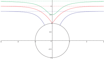
Figure 1: A brane interacting with a black hole: The round circle is the black hole horizon. We schematically show the profiles of the brane for 3 different cases. The brane which touches the horizon at one point and has a cone-like profile near it is critical. Two other solid lines show branes close to the critical one. One of them (sub-critical) does not intersect the horizon, while the other (super-critical) one crosses the horizon at the spherical surface with a small radius $R_{0}$. At far distance the brane surfaces are parallel to the equatorial plane of the black hole.

We consider sub-critical and super-critical solutions as two different phases of the BBH-system. Let us consider a continuous deformation of solutions during which a solution transits from one phase to another. If we parametrize these solutions by a parameter $\lambda$, there exists a special value of it, $\lambda=\lambda_{*}$, where the phase is changed. We call the corresponding solution critical. ( Figure 1 schematically shows the critical and near critical solutions for this process.) We focus our attention on the solutions close to the critical one and study the properties of the BBH-system during the merger transition when the solution changes its phase.

IV Brane configurations near the horizon

Near the horizon the coefficient $F$ of the bulk metric has the form

$$F\approx 2\kappa(r-r_{0})+O((r-r_{0})^{2})\,,$$ (21)

where $\kappa={1\over 2}(dF/dr)|_{r_{0}}$ is the surface gravity. To study the near-horizon behavior of the brane it is convenient to introduce the proper distance coordinate

$$Z=\int_{r_{0}}^{r}{dr\over\sqrt{F}}\,.$$ (22)

In the vicinity of the horizon one has

$$r-r_{0}\approx\kappa Z^{2}/2\,,\hskip 14.22636ptF\approx\kappa^{2}Z^{2}\,.$$ (23)

We are interested in the case when a ‘central’ part of the brane is located in the close vicinity of the horizon or crosses it. In the latter case, we assume that the radius $R_{0}$ of the surface of the intersection of the brane with the bulk horizon is much smaller than the size of the horizon $r_{0}$. Under these conditions one can approximate the spaceime close to the bulk black hole horizon by the Rindler space where the horizon is a $(n+1)$-dimensional plane. In this approximation the metric (1) takes the form

$$dS^{2}=-\kappa^{2}Z^{2}dT^{2}+dZ^{2}+dL_{N-2}^{2}\,,$$ (24)

where $dL_{N-2}^{2}$ is the metric of $(N-2)$-dimensional Euclidean space ${\mathbb{E}}^{N-2}$. We write $dL_{N-2}^{2}$ in the form

$$dL_{N-2}^{2}=dY^{2}_{D}+\ldots+dY^{2}_{N-2}+dR^{2}+R^{2}d\Omega^{2}_{D-2}\,,$$ (25)

and choose the Cartesian coordinates $Y$ so that the equation (7) takes the form $Y_{D}=\ldots=Y_{N-2}=0$, while the brane equation is

$$F(Z,R)=0\,.$$ (26)

We write a solution of this equation in a parametric form

$$Z=Z(\lambda)\,,\hskip 14.22636ptR=R(\lambda)\,.$$ (27)

Then the induced metric on the brane is

$$ds^{2} = -\kappa^{2}Z^{2}dT^{2}$$ (28)

$$+ [(dZ/d\lambda)^{2}+(dR/d\lambda)^{2}]d\lambda^{2}+R^{2}d\Omega^{2}_{n}\,.$$

Here, as earlier, $n=D-2$. The action (5) for this induced metric takes the form

$$S=\kappa\Delta T{\cal A}_{n}{\cal S}\,,$$ (29)

$${\cal S}=\int d\lambda ZR^{n}\sqrt{(dZ/d\lambda)^{2}+(dR/d\lambda)^{2}}\,.$$ (30)

This action is evidently invariant under a reparametrization $\lambda\to\tilde{\lambda}(\lambda)$. In the regions where either $Z$ or $R$ is a monotonic function of $\lambda$, these functions themselves can be used as parameters. As a result, one obtains two other forms of the action which are equivalent to ${\cal S}$

$${\cal S}=\int dZ{\cal L}_{R}=\int dR{\cal L}_{Z}\,,$$ (31)

where

$${\cal L}_{R}=ZR^{n}\sqrt{1+{R^{\prime}}^{2}}\,,\hskip 14.22636pt{\cal L}_{Z}=ZR^{n}\sqrt{1+{\dot{Z}}^{2}}\,.$$ (32)

Here the prime means the derivative with respects to $Z$, while the dot stands for the derivative with respect to $R$. The corresponding Euler-Lagrange equations are

$$ZRR^{\prime\prime}+(RR^{\prime}-nZ)(1+{R^{\prime}}^{2})=0\,.$$ (33)

$$RZ\ddot{Z}+(nZ\dot{Z}-R)(1+{\dot{Z}}^{2})=0\,.$$ (34)

It is easy to check that the form of the equation (33) is invariant under the following transformation

$$R(Z)=k\tilde{R}(\tilde{Z})\,,\hskip 14.22636ptZ=k\tilde{Z}\,.$$ (35)

Similarly, the transformation

$$Z(R)=k\tilde{Z}(\tilde{R})\,,\hskip 14.22636ptR=k\tilde{R}$$ (36)

preserves the form of (34).

To obtain the boundary conditions to the equations (33) and (34) we require that the induced metric on the brane is regular. This implies that the curvature invariants are regular as well. Let us consider the scalar curvature of the induced metric, which we denote by ${\cal R}$. For the brane parametrization $R=R(Z)$ the induced metric is

$$ds^{2}=-\kappa^{2}Z^{2}dT^{2}+[1+{R^{\prime}}^{2}]dZ^{2}+R^{2}d\Omega^{2}_{n}\,,$$ (37)

and the corresponding scalar curvature takes the form

$${\cal R}={\cal R}^{(2)}+{n(n-1)\over R^{2}}-2n{\Box^{(2)}R\over R}-n(n-1){(\nabla R)^{2}\over R^{2}}\,.$$ (38)

The quantities in the right-hand side of this relation are calculated for the two-dimensional metric which is the metric of the $(T-Z)$-sector of the (28). In particular, ${\cal R}^{(2)}$ is the two-dimensional curvature of this metric. Calculating ${\cal R}$ and using the brane equation (33) to exclude the second derivatives $d^{2}R/dZ^{2}$ one gets

$${\cal R}={2R^{2}{R^{\prime}}^{2}-6nZRR^{\prime}+n(3n-1)Z^{2}\over Z^{2}R^{2}(1+{R^{\prime}}^{2})}\,.$$ (39)

Simple analysis shows that if the brane crosses the horizon of the bulk black hole, then the regularity of ${\cal R}$ on the horizon requires

$$R|_{Z=0}=R_{0}\,,\hskip 14.22636pt\left.{dR\over dZ}\right|_{Z=0}=0\,.$$ (40)

By using (33) one obtains that for this solution near the horizon one has

$$R=R_{0}+{nZ^{2}\over 4R_{0}}+\ldots\,.$$ (41)

For a brane which does not cross the horizon one has $Z(R=0)>0$, and at this point one has $R^{\prime}\to\infty$. This gives the following boundary conditions

$$Z|_{R=0}=Z_{0}\,,\hskip 14.22636pt\left.{dZ\over dR}\right|_{R=0}=0\,.$$ (42)

These conditions can also be obtained from the regularity of ${\cal R}$ in the parametrization $Z=Z(R)$. Using (34) one gets

$$Z=Z_{0}+{R^{2}\over 2(n+1)Z_{0}}+\ldots\,.$$ (43)

One can check that when the condition of regularity of the Ricci scalar is satisfied, the other curvature invariants are also finite.

A solution near the horizon (either (40) or (42)) determines uniquely a global solution of the brane equation (12). Thus for a given small value of $R_{0}$ ($Z_{0}$) the asymptotic data of the corresponding solution, $\{p,p^{\prime}\}$, are uniquely determined and are continuous functions of $R_{0}$ ($Z_{0}$).

V Critical solutions as attractors

The equations (33)-(34) have a simple solution

$$R=\sqrt{n}Z$$ (44)

which plays a special role. We call it a critical solution. It describes a critical brane which touches the horizon of the bulk black hole at one point, $Z=R=0$. The critical solution separates two different families of solutions (phases), super-critical and sub-critical. Let us show that the critical solution is an attractor, and solutions of the both families are attracted to the critical solution asymptotically.

To do this, we, following flc , introduce new variables

$$x=R^{\prime}\,,\hskip 5.69046pty=Z^{-1}RR^{\prime}\,,\hskip 5.69046ptds=dZ/(yZ)\,.$$ (45)

In these variables the equation (33) can be written in the form of the first order regular autonomous system

$${dx\over ds} = x(n-y)(1+x^{2})\,,$$ (46)

$${dy\over ds} = y[n-2y+x^{2}(n+1-y)]\,.$$ (47)

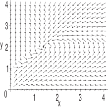
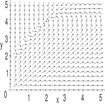
Figure 2: Phase portraits of the system (46)-(47) for $n=2$ (left plot) and for $n=4$ (right plot).

The critical points on the phase space $(x,y)$ are the points where the right-hand side of the both equations (46) and (47) vanish simultaneously. These critical points are: a node, $(0,0)$; a saddle point, $(0,n/2)$, and two focus points, $(\pm\sqrt{n},n)$. For different $n$ the phase portrait are similar. The Figure 2 shows the phase portraits for $n=2$ and $n=4$, which have the focus points at $(\sqrt{2},2)$ and $(2,4)$, respectively. The focus points are attractors, and they correspond to the critical solutions $R=\sqrt{n}Z$.

VI Near-critical solutions in the vicinity of the horizon

Let us consider now solutions which are close to the critical one

$$R=\sqrt{n}Z+\rho(Z)\,.$$ (48)

Substituting this expression into (33), and keeping linear in $\rho$ terms we obtain

$$Z^{2}\rho^{\prime\prime}+(n+1)Z\rho^{\prime}+(n+1)\rho=0\,.$$ (49)

A solution of this equation is of the form

$$\rho=Z^{\beta}\,,\hskip 14.22636pt\beta_{\pm}={1\over 2}(-n\pm\sqrt{n^{2}-4n-4})\,.$$ (50)

The parameter $n$ is a positive integer. For $n\leq 4<2(1+\sqrt{2})$ the exponent $\beta$ is complex, while for $n\geq 5$ it is real.

Let us consider first the case of complex $\beta$, that is when the number of the brane spaceime dimensions is $D\leq 6$. We write a near-critical solution (48) in the form

$$R=\sqrt{n}Z+Z^{-n/2}\Re(CZ^{i\alpha})\,,$$ (51)

where $C$ is a complex number and $\alpha={1\over 2}\sqrt{4+4n-n^{2}}$. The initial data $R(Z=0)=R_{0}$ determines the factor $C$. We denote the corresponding values of it by $C(R_{0})$. Under the scaling transformation (35) the surface $Z=0$ is invariant, while $R_{0}$ is transformed into $\tilde{R}_{0}=k^{-1}R_{0}$. Using (51) we obtain

$$C(kR_{0})=k^{-1-n/2+i\alpha}C(R_{0})\,.$$ (52)

For $D\geq 7$ the both exponents $\beta_{\pm}$ are real and one has $\beta_{+}\beta_{-}=4(n-1)$, so that both $\beta_{\pm}$ are negative. The critical solution (44) is again the attractor and one has

$$R=\sqrt{n}Z+C_{+}Z^{\beta_{+}}+C_{-}Z^{\beta_{-}}\,.$$ (53)

Using again the arguments based on the scaling properties of the equation (33) one can conclude that $C_{\pm}$ considered as functions of $R_{0}$ obey the properties

$$C_{\pm}(kR_{0})=k^{\beta_{\pm}-1}C_{\pm}(R_{0})\,.$$ (54)

Similarly, one can consider near-critical solutions of the equation (34). Let us write

$$Z={1\over\sqrt{n}}R+\zeta(R)\,.$$ (55)

Then keeping linear in $\zeta$ terms one obtains

$$R^{2}\ddot{\zeta}+(n+1)R\dot{\zeta}+(n+1)\zeta=0\,.$$ (56)

It has the same form and the same coefficients as the equation (49). For this reason, as it can be expected, the critical dimension and the scaling property (35) are the same for the both linearized equations.

VII Scaling and self similarity

Since near the horizon the equation (12) reduces to (33), one can uniquely define a special global solution of (12) which near the horizon reduces to the critical solution (44). This critical solution near the horizon is of the form rem

$$\theta\approx\sqrt{{2n(r-r_{0})\over\kappa r_{0}^{2}}}\,.$$ (57)

Being traced to infinity, the critical solution determines uniquely the asymptotic data $\{p,p^{\prime}\}$ which we denote by $\{p_{*},p^{\prime}_{*}\}$, respectively. If the function $F(r)$ in the metric is given one can find $\{p_{*},p^{\prime}_{*}\}$, for example, by solving the equation (12) numerically.

Consider a super-critical solution. For this solution the radius $R_{0}$ of the horizon of the brane black hole is connected with $\theta_{0}$ as follows $R_{0}=r_{0}\sin\theta_{0}$. For small $\theta_{0}$ one has $R_{0}=r_{0}\theta_{0}$. We denote by $\{p,p^{\prime}\}$ the asymptotic data for a solution with a given $R_{0}$. For the critical solution, $R_{0}=0$, the asymptotic data are $\{p_{*},p^{\prime}_{*}\}$. We also denote $\Delta p=\sqrt{(p-p_{*})^{2}+(p^{\prime}-p^{\prime}_{*})^{2}}$. Similarly, one can define $\Delta p$ for sub-critical solutions. In the both cases for the critical solution, and only for it, $\Delta p=0$ . One can use $\Delta p$ as a measure indicating how close a solution is to the critical one. Our goal is to demonstrate that $R-0$ (or $Z_{0}$) considered as a function of $\Delta p$ has a self-similar behavior. We shall show that there exists a critical dimension, $D_{*}$, such that for $D>D_{*}$ this symmetry is continuous, while for $D\leq D_{*}$ it is discrete. This critical dimension for the BBH-system is $D_{*}=6$. It should be emphasized that in the definition one can use any positive definite quadratic form of $p-p_{*}$ and $p^{\prime}-p^{\prime}_{*}$ of $\Delta p$ instead of $(p-p_{*})^{2}+(p^{\prime}-p^{\prime}_{*})^{2}$. It can be checked that this does not change the result.

VII.1 $D\leq 6$ case

Since in the solution (44) is the attractor, both sub-critical and super-critical solutions which are close to the critical solution in the vicinity of the horizon remain close to it everywhere. This implies that the difference between the near-critical and critical solutions is small and it can be obtained by solving a linear equation. For this equation both $(p-p_{*},p^{\prime}-p^{\prime}_{*})$ and the complex coefficient $C$ in (51) are uniquely defined by $R_{0}$, so that there exists a linear relation between these coefficients

$$C=a(p-p_{*})+b(p^{\prime}-p^{\prime}_{*})\,,\ \bar{C}=\bar{a}(p-p_{*})+\bar{b}(p^{\prime}-p^{\prime}_{*})\,,$$ (58)

where $a$ and $b$ are complex numbers. Substituting $\{p,p^{\prime}\}$ obtained from these equations into the definition of $\Delta p$ one gets

$$(\Delta p)^{2} = P^{2}\left[C\bar{C}-\bar{{\cal A}}C^{2}-{\cal A}{\bar{C}}^{2}\right]\,,$$ (59)

$${\cal A} = |{\cal A}|e^{iA}={a^{2}+b^{2}\over 2(|a|^{2}+|b|^{2})}\,,$$ (60)

$$P^{2} = -{2(|a|^{2}+|b|^{2})\over(a\bar{b}-\bar{a}b)^{2}}\,.$$ (61)

It is easy to show that $P^{2}$ is non-negative, and

$$|{\cal A}|\leq 1/2\,.$$ (62)

In the latter relation the equality takes place when $a/\bar{a}=b/\bar{b}$. This is a degenerate case and by a small change of the bulk metric this condition will be violated. Thus we assume that $|{\cal A}|<1/2$.

We denote by $\Delta\tilde{p}$ and $\tilde{C}$ quantities which correspond to the solution with $R=\tilde{R}_{0}$. Then one has

$${(\Delta p)^{2}\over(\Delta\tilde{p})^{2}}={C\bar{C}-\bar{{\cal A}}C^{2}-{\cal A}{\bar{C}}^{2}\over\tilde{C}\bar{\tilde{C}}-\bar{{\cal A}}\tilde{C}^{2}-{\cal A}{\bar{\tilde{C}}}^{2}}\,.$$ (63)

The scaling transformation (35) maps $Z=0$ onto itself, and hence it preserves the position of the horizon, while it changes the value of $R_{0}$. Let us choose $k=R_{0}/\tilde{R}_{0}$, then, using (52), one has

$$C=(R_{0}/\tilde{R}_{0})^{(n+2)/2-i\alpha}\tilde{C}\,,\hskip 14.22636pt\gamma=1+n/2\,.$$ (64)

Let us denote

$${\cal B}={\cal A}{\bar{\tilde{C}}\over\tilde{C}}=|{\cal A}|e^{iB}\,.$$ (65)

Then one has

$${(\Delta p)^{2}\over(\Delta\tilde{p})^{2}}={R_{0}^{n+2}\,[1-2|{\cal A}|\cos(2\alpha\ln R_{0}+B^{\prime})]\over\tilde{R}_{0}^{n+2}\,[1-2|{\cal A}|\cos(B)]}\,,$$ (66)

where $B^{\prime}=B-2\alpha\ln\tilde{R}_{0}$. It follows from this relation that

$$\ln(\Delta p) = {n+2\over 2}\ln R_{0}+H$$ (67)

$$+ {1\over 2}\ln[1-2|{\cal A}|\cos(2\alpha\ln R_{0}+B^{\prime})]\,,$$

where $H$ and $B^{\prime}$ do not depend on $R_{0}$.

For small $R_{0}$ the leading part of this equation gives

$$\ln R_{0}\sim{2\over n+2}\ln(\Delta p)\,.$$ (68)

Using this relation and iterating (67) one obtains

$$\ln R_{0}\sim\gamma\ln(\Delta p)+f(\ln(\Delta p))+C\,.$$ (69)

Here $C$ is a constant,

$$\gamma={2\over n+2}\,,$$ (70)

and $f(z)$ is a periodic function of $z$, $f(z+\omega)=f(z)$ with the period $\omega$

$$\omega={\pi(n+2)\over\sqrt{4+4n-n^{2}}}\,.$$ (71)

For $n=1$ relations (70) and (71) reproduce the result obtained in cfl ; flc .

VII.2 $D>6$ case

In this case the real coefficients $C_{\pm}$ are connected with the asymptotic data $\{p,p^{\prime}\}$ as follows

$$p-p_{*}=a_{+}C_{+}+a_{-}C_{-}\,,\hskip 5.69046ptp^{\prime}-p^{\prime}_{*}=a^{\prime}_{+}C_{+}+a^{\prime}_{-}C_{-}\,,$$ (72)

and one has

$$(\Delta p)^{2} = (a_{+}^{2}+{a^{\prime}_{+}}^{2})C_{+}^{2}+(a_{-}^{2}+{a^{\prime}_{-}}^{2})C_{-}^{2}$$ (73)

$$+ 2(a_{+}a_{-}+a^{\prime}_{+}a^{\prime}_{-})C_{+}C_{-}\,.$$

The equation (54) implies

$$C_{\pm}=\left({R_{0}\over\tilde{R}_{0}}\right)^{1-\beta_{\pm}}\tilde{C}_{\pm}\,.$$ (74)

Since $a_{+}^{2}+{a^{\prime}_{+}}^{2}$ does not vanish and $1-\beta_{\pm}>0$, $1-\beta_{+}<1-\beta_{-}$, the first term in the right hand side of the relation (73) is the leading one for small $R_{0}$. $(\Delta p)^{2}$ as a function of $R_{0}$ has the following asymptotic form for small $R_{0}$

$$\ln(\Delta p)^{2}\sim 2(1-\beta_{+})\ln R_{0}\,.$$ (75)

Or, equivalently, one has

$$\ln R_{0}\sim\gamma\ln(\Delta p)\,,\hskip 5.69046pt\gamma={n+2+\sqrt{n^{2}-4n-4}\over 4(n+1)}\,.$$ (76)

Hence for the number of dimensions higher than the critical one has the scaling law (76). The sub-leading oscillations are absent and the symmetry is continuous.

The relations (69)-(71) and (76) demonstrate the scaling law for the super-critical solutions close to the critical one. It is easy to check that similar relations are valid for sub-critical solutions as well.

VIII Merger transitions: Inside brane story

Let us imagine that there is an observer ‘living’ within the brane who is not aware of the existence of the bulk extra-dimensions. Let us discuss what happens from his or her point of view when the BBH-system changes its phase. As earlier we consider a one-parameter family and assume that the merger transition occurs at the special value of the parameter $\lambda=\lambda_{*}$. From the point of view of the brane observer this family describes a process in which a brane black hole is either created or destroyed. The surface gravity of the brane black hole always coincides with the surface gravity $\kappa$ of the bulk black hole, and hence it remains constant during this process. For the description of the transition it is convenient to make the Wick’s rotation $T\to i\tau$ and to choose the Euclidean time $\tau$ to have the period $\kappa/(2\pi)$. In such (‘canonical’ by the terminology adopted in kol ) approach the Euclidean topology of the BBH-system in two different phases is different. Namely, for family of sub-critical solutions the topology is $S^{1}\times R^{D-1}$, while for the super-critical solutions the topology is $R^{2}\times S^{D-2}$. Following kol , we call such a topology change transition the merger transition.

The internal geometry of the brane is determined by its embedding into the bulk spacetime. But if the brane observer does not know about the existence of extra-dimensions, he/she may try to use the ‘standard’ $D$-dimensional Einstein equations in order to interpret the observed brane geometry. Such an observer would arrive to the conclusion that the brane spacetime is not empty and there exists a distribution of the matter in it. By using the $D$-dimensional Einstein equations

$$G_{ab}=R_{ab}-{1\over 2}\gamma_{ab}R={\cal T}_{ab}\,,\hskip 14.22636pt{\cal T}_{ab}=8\pi T_{ab}$$ (77)

one can obtain the corresponding effective stress-energy tensor $T_{ab}$. (We use units in which the $D$-dimensional gravitational coupling constant is $1$.) To calculate $G_{ab}$ we write the induced metric on the brane (8) in the form ($A,B=(0,1)$)

$$ds^{2}=\gamma_{ab}d\zeta^{a}d\zeta^{b}=h_{AB}dy^{A}dy^{B}+\rho^{2}(y)d\Omega_{n}^{2}\,.$$ (78)

The symmetry of the metric (78) implies that ${\cal T}_{a}^{b}$ has the following non-vanishing components

$${\cal T}^{b}_{a}=\left(\begin{array}[]{ccccc}{\cal T}^{0}_{0}&{\cal T}^{0}_{1}&0&\ldots&0\\ {\cal T}^{0}_{1}&{\cal T}^{1}_{1}&0&\ldots&0\\ 0&0&\hat{\cal T}&\ldots&0\\ \ldots&\ldots&\ldots&\ldots&\ldots\\ 0&0&0&\ldots&\hat{\cal T}\end{array}\right).$$ (79)

The calculations give

$${\cal T}_{AB} = n\left[-{\rho_{:AB}\over\rho}+\left({\Box^{(2)}\rho\over\rho}+\displaystyle\frac{n-1}{2\rho^{2}}{\cal P}\right)h_{AB}\right]\,,$$

$$\hat{{\cal T}} = (n-1)\left[{\Box^{(2)}\rho\over\rho}+\displaystyle\frac{n-2}{2\rho^{2}}{\cal P}\right]-{1\over 2}\,{\cal R}^{(2)},$$

where ${\cal P}=(\nabla\rho)^{2}-1$.

For the super-critical solutions, substituting (41) into (VIII) one obtains at the horizon ($Z=0$)

$${\cal T}_{T}^{T}={\cal T}_{Z}^{Z}={n\over 2R_{0}^{2}}\,,\hskip 14.22636pt\hat{{\cal T}}={n^{2}+2n-4\over 4R_{0}^{2}}\,.$$ (81)

Similarly, for the sub-critical solutions, substituting (43) into (VIII) one obtains at the top of the brane ($R=0$)

$${\cal T}_{T}^{T}=-{n\over 2(n+1)Z_{0}^{2}}\,,\hskip 5.69046pt{\cal T}_{R}^{R}=\hat{{\cal T}}={n(n+3)\over 2(n+1)^{2}Z_{0}^{2}}\,,$$ (82)

The equations (81) and (82) show that in the both phases the tensor $T_{a}^{b}$ calculated at the horizon respects the symmetries of the induced metric.

IX Discussion

We discussed merger transitions in the brane–black-hole system. We would like to emphasize that there exists a striking similarity between this phenomenon and the merger transitions in the black-hole–black-string system kol ; kol1 . Namely, close to the horizon the near critical solutions of the BBH-system has the same ‘double cone’ structure as the solutions for the merger transition of the caged black holes. The equations defining the near critical solutions, following from the Einstein action for the latter system, and the equations for the BBH-system are very similar. In both cases there is a critical dimension of the spacetime where the scaling parameter $\alpha$ becomes real. For $D=3$, the parameter $\alpha$ is the same in the both cases.

Kol kol discussed a possible relation between merger transitions and the Choptuik phenomena. This similarity with the critical collapse takes place in the BBH-system as well. To demonstrate this let us consider a slow evolution of the BBH-system in time which starts with no-brane-black-hole, so that a black hole is formed as a result of time evolution. As earlier, one has a one-parameter family of quasi-static configurations, and at the moment of brane-black-hole formation the asymptotic data $(\{p,p^{\prime}\})$ reaches the critical value $(\{p_{*},p_{*}^{\prime}\})$. The relations (82) show that the curvature at the center of the brane is growing until it formally becomes infinite at the moment of the black hole formation. For $D\leq 6$ the growing of the curvature is periodically modulated as it happens in the critical collapse case GD ; GCD . For the number of dimensions higher than the critical one (for $D>6$) this oscillatory behavior disappears. The scaling laws, relating the size $R_{0}$ of the formed brane-black-hole with $\Delta p$, also has the same scaling and self-similar behavior as in the critical collapse case chop .

In our analysis we focused on the static brane solutions and neglected the effects connected with the brane tension. Let us discuss what happens when the brane is moving. If the brane approaches the bulk black hole the BBH will be created. In the inverse case when the brane, initially crossing the bulk black hole horizon, is moving away from the black hole, the BBH can disappear. In a general case, for finite velocity of the brane one cannot use the adiabatic approximation and describe the brane motion as a set of static configurations. To study dynamics of this process one needs to include a time variable explicitly and to solve a 2-dimensional problem. This can be done numerically. In many aspects this problem is similar to (but more complicated than) numerical solving of equations for moving cosmic strings interacting with the bulk black hole SFV ; SF . Let us emphasize that the dynamics of the process of BBH disappearance is not a time reversed version of the BBH formation process.

The reason of this time asymmetry is connected with the presence of the bulk black hole. Consider a bulk black hole formed as a result of the gravitational collapse of some matter. By definition, the black hole is a region of the bulk spacetime causally disconnected from the future null infinity. A solution obtained by inversion of the direction of time $t\to-t$ describes a completely different physical process, an expansion of the matter from the white black hole (see e.g. FN ). Physical processes in the spacetime of a black hole obey natural condition of regularity at the future event horizon. To study such processes in the spacetime of a black hole long time after its formation one can ”forget” about the details of the gravitational collapse and to use the eternal black hole approximation imposing the same regularity conditions at the future event horizon. For a static solutions this regularity conditions imply its regularity at the past horizon of the eternal black hole. For time-dependent configurations in a general case this is not true.

Interaction of a moving brane with the black hole was studied numerically in FT ; FPSTa ; FPSTb . A main motivation for this study is connected with the following question: under which conditions a black hole moving with some velocity can escape from the brane FSa ; FSb . By solving numerically test brane equations in a spacetime of a static black hole it was shown FT that in the considered cases a moving brane is bend and eventually the radius of the pinched part goes to zero. This indicates that the extraction of the test brane from the bulk black hole is accompanied by its reconnection FT . After the reconnection a peace of the brane near the horizon (”a baby brane”) is absorbed by the black hole, while the other part, located outside of the black hole (”a mother brane”), keeps moving away from the black hole. In such a process a brane observer registers that the BHH disappears at the moment of the reconnection.

In the limit of small velocity of the brane, effects connected with the brane tension cannot be ignored and they can significantly change the dynamics of the system. Consider a $D$-dimensional brane with the tension $\sigma$ in the spacetime of $N$-dimensional black hole with the gravitational radius $r_{0}$. For these parameters one can construct the following dimensionless combination $\epsilon=G^{N}\sigma/r_{0}^{N-D-2}$, where $G^{N}$ is the Newtonian coupling constant in the bulk spacetime. It is argued in FT ; FPSTb that the escape velocity for such a system is of the order of $\epsilon^{1/2}$.

In the above discussion we assumed that the brane is infinitely thin. In the field theory with the spontaneous symmetry breaking the brane-like objects (e.g domain walls) arise as a solution of non-linear equations, and they have finite thickness. Static thick domain walls interacting with a black hole were studied in MYIIN ; MIIK ; Rog ; MRa ; MRb .

One can expect that for an infinitely thin brane in the process of its reconnection, during which the BBH disappears,the curvature of the induced metric infinitely grows as it happens for the critical solutions discussed above. Under these conditions one cannot neglect the finite thickness effect. One can expect that formal singularities in the infinitely thin brane description would disappear when one uses a (more fundamental) field theory description. In this connection the recent numerical calculations performed in FPST are very stimulating. It is interesting to analyze in more details the dynamics of the destruction of BBHs in the framework of the field theory models. For a finite-thickness brane a choice of the surface, which represents it, is not unique. Thus for the thick brane the meaning of the induced geometry is not well defined. If the gravity is emergent phenomenon the merger and topology change transitions in the physical spacetime might have similar features with those of the discussed toy model. Namely in the vicinity of these transitions one cannot any more use the metric for the description of the details of the transition. Instead a more detailed microscopic description in terms of constituents (e.g. strings) is required. The toy model proposed in this paper and its field theory analogues might be useful for modeling these transitions.

References

- (1) T. Harmark and N. A. Obers, Phases of Kaluza-Klein black holes: A brief review, e-print hep-th/0503020 (2005).
- (2) B. Kol, The phase transition between caged black holes and black strings: A review, eprint hep-th/0411240 (2004).
- (3) B. Kol, Choptuik scaling and the merger transitions, e0print hep-th/0502033 (2005).
- (4) M. W. Choptuik, Phys. Rev. Lett. 70, 9 (1993).
- (5) G. T. Horowitz, Class. Quant. Grav. 8, 587 (1991).
- (6) P. A. M. Dirac, Proc. Royal Soc. London A268, 57 (1962).
- (7) J. Nambu, Copenhagen Summer Symposium (1970), unpublished; T. Goto, Prog. Theor. Phys. 46, 1560 (1971).
- (8) V. P. Frolov, M. Snajdr, and D. Stojkovic, Phys. Rev. D68, 044002 (2003).
- (9) M. Kruczenski, D. Mateos, R. C. Myers, D. J. Winters, JHEP 0405:041 (2004), eprint hep-th/0311270.
- (10) M. Christensen, V. P. Frolov, and A. L. Larsen, Phys. Rev. D58, 085005 (1998).
- (11) V. P. Frolov, A. L. Larsen, and M. Christensen, Phys. Rev. D59, 125008 (1999).
- (12) F. R. Tangherlini, Nuovo Cimento, 77, 636 (1963).
- (13) This asymptotic cannot be obtained by a continuous transition in (16). The reason is that at the horizon the coefficients and in the equation (12) diverge and hence the corresponding terms which were not important for a sub-critical solution (16) cannot be neglected for the critical solution.
- (14) D. Garfinkle, G. C. Duncan, Phys. Rev. D58, 064024 (1998).
- (15) D. Garfinkle, C. Cutler, and G. C. Duncan, Phys. Rev. D60, 104007 (1999).
- (16) I would like to use this opportunity to thank again Arne Larsen for our many fruitful discussions which were very stimulating for the writing this paper.
- (17) M. Snajdr, V. P. Frolov, and J.-P. DeVilliers, Class. Quant. Grav. 19, 5987 (2002).
- (18) M. Snajdr and V. P. Frolov, Class. Quant. Grav. 20, 1303 (2003).
- (19) V. Frolov and I. Novikov. Black Hole Physics: Basic Concepts and New Developments (Kluwer Academic Publ.), 1998.
- (20) A. Flachi and T. Tanaka, Phys. Rev. Lett. 95, 161302 (2005).
- (21) A. Flachi, O. Pujolas, M. Sasaki, T. Tanaka, Phys. Rev. D73, 125017 (2006).
- (22) A. Flachi, O. Pujolas, M. Sasaki, T. Tanaka, Critical escape velocity of black holes from branes, e-Print hep-th/0604139 (2006).
- (23) V. Frolov and D. Stojkovic, Phys. Rev. Lett. 89, 151302 (2002).
- (24) V. Frolov and D. Stojkovic, Phys. Rev. D66, 084002 (2002).
- (25) Y. Morisawa, R. Yamazaki, D. Ida, A. Ishibashi, K.-I. Nakao, Phys. Rev. D62, 084022 (2000).
- (26) M. Rogatko, Phys. Rev. D64, 064014 (2001).
- (27) R. Moderski and M. Rogatko, Phys. Rev. D69, 084018 (2004).
- (28) R. Moderski and M. Rogatko, Phys. Rev. D67, 024006 (2003).
- (29) Y. Morisawa, D. Ida, A. Ishibashi, K.-I. Nakao, Phys. Rev. D67, 025017 (2003).
- (30) A. Flachi, O. Pujolas, M. Sasaki, T. Tanaka, Dynamics of Domain Walls Intersecting Black Holes, e-Print hep-th/0601174 (2006).