Spin Dependence in Computational Black Hole Data

Abstract

We have implemented a parallel multigrid solver, to solve the initial data problem for $3+1$ General Relativity. This involves solution of elliptic equations derived from the Hamiltonian and the momentum constraints. We use the conformal transverse-traceless method of York and collaborators YP ; MY ; York ; Mathews ; Bowen+York which consists of a conformal decomposition with a scalar $\phi$ that adjusts the metric, and a vector potential $w^{i}$ that adjusts the longitudinal components of the extrinsic curvature. The constraint equations are then solved for these quantities $\phi$, $w^{i}$ such that the complete solution fully satisfies the constraints. We apply this technique to compare with theoretical expectations for the spin-orientation- and separation-dependence in the case of spinning interacting (but not orbiting) black holes. We write out a formula for the effect of the spin-spin interaction which includes a result of Wald WaldPRD as well as additional effect due to the rotation of the mass quadrupole moment of a spinning black hole. A subset of these spin-spin effects are confirmed via our numerical calculations, however due to computer time limitations the full parameter space has not yet been surveyed and confirmed. In particular, at the relatively small separations ($d\leq 18m$) we are able to consider, we are unable to confirm the expected asymptotic fall-off of $d^{-3}$ for these effects.

Keywords: numerical relativity; spin-spin coupling; black hole initial data.

1 Introduction

Simulation of binary black hole mergers will play an important part in the prediction, detection, and the analysis of signals in gravitational wave detectors. In the usual approach to computing the merger of black holes (generically called the $3+1$ method), one has first to initiate the simulation by producing consistent data. Four of the components of the Einstein equation do not contain time derivatives of the spatial metric, nor of the momentum of the 3-metric. These components, $G_{00}=0$ and $G_{i0}=0$, are thus called constraint equations, and they must be satisfied in any specification of initial data. (We are interested in black hole interactions, which are vacuum, i.e. matter-free, so the right side of the Einstein equation is zero: $G_{\mu\nu}=0$.) As we recall in the next section, a conformal decomposition YP ; MY ; York ; Mathews ; Bowen+York ; Choquet ; Lichnerowicz allows the solution of these components to be put in the form of a set of four coupled elliptic equations. These elliptic equations are the subject of our work. We solve them via a multigrid method which applies concepts from Hawley+Matzner to this problem. We demonstrate the accuracy of our data by considering features discussed analytically by Wald WaldPRD . Wald described the spin-spin effect on the binding energy of two black holes in an analytic perturbation scheme, where one hole is much more massive than the other. Our computational technology is well suited to simulating these effects for equal mass black holes, and we demonstrate agreement in some aspects of the computational spin-spin interactions with the analytic estimate, for separations that are not small.

2 $3+1$ Formulation of Einstein Equations

We take a Cauchy formulation (3+1) of the ADM type, after Arnowitt, Deser, and Misner ADM . In such a method the 3-metric $g_{ij}$ and its momentum $K_{ij}$ are specified at one initial time on a spacelike hypersurface, and evolved into the future. The ADM metric is

$${\rm d}s^{2}=-(\alpha^{2}-\beta_{i}\beta^{i})\,{\rm d}t^{2}+2\beta_{i}\,{\rm d}t\,{\rm d}x^{i}+g_{ij}\,{\rm d}x^{i}\,{\rm d}x^{j}$$ (1)

where $\alpha$ is the lapse function and $\beta^{i}$ is the shift 3-vector; these gauge functions encode the coordinatization.†

The Einstein field equations contain both hyperbolic evolution equations and elliptic constraint equations. The constraint equations for vacuum in the ADM decomposition are:

$$H=\frac{1}{2}[R-K_{ij}K^{ij}+K^{2}] = 0,$$ (2)

$$H^{i}=\nabla_{j}\left(K^{ij}-g^{ij}K\right) = 0.$$ (3)

Eq. (2) is known as the Hamiltonian constraint; Eq. (3) is the momentum constraint (three components). Here $R$ is the 3-d Ricci scalar constructed from the 3-metric, and $\nabla_{j}$ is the torsion-free 3-d covariant derivative compatible with $g_{ij}$. Initial data must satisfy these constraint equations; one may not freely specify all components of $g_{ij}$ and $K_{ij}$.

One of the evolution equations from the Einstein system is

$$\dot{g}_{ij}=-2\alpha K_{ij}+\nabla_{j}\beta_{i}+\nabla_{i}\beta_{j},$$ (4)

and this will prove useful in our data setting procedure below.

3 Data Form

Solutions of the initial value problem have been addressed in the past by several groups,  YP ; MY ; York ; Mathews ; Bowen+York ; Choquet ; Lichnerowicz ; Hawley+Matzner ,  Cook ; Pfeiffer ; Baumgarte ; GGB1 ; GGB2 ; GGB3 ; Cook2 ; Pfeiffer2 ; CookReview ; Shoemaker ; Huq . It is the case that until recently, most data have been constructed assuming that the initial 3-space is conformally flat. The method most commonly used is the approach of Bowen and York Bowen+York , which chooses maximal spatial hypersurfaces (for which the quantity $K\equiv{K^{a}}_{a}=0$), as well as taking the spatial 3-metric to be conformally flat.

The chief advantage of the maximal spatial hypersurface approach is numerical simplicity, as this choice decouples the Hamiltonian constraint from the momentum constraint equations. Besides, for $K=0$, if the conformal background is flat Euclidean 3-space, then there are known $K_{ij}$ that analytically solve the momentum constraint Bowen+York . The constraints then reduce to one elliptic equation for the conformal factor $\phi$. Very recently substantial success has been achieved evolving Bowen-York data using “puncture” methods Brownsville ; Goddard . However, we generally use an alternative choice of background 3-metric, which is based on a metric constructed from single black hole Kerr Schild dataKerrSchild ; multiple black holes are constructed by a superposition in the conformal background. It has been shown that this process, while not exact for multiple black hole data, does contain much of the physics. It clearly is exact for a single black hole, even a spinning or boosted black hole Matzner:1999pt .

3.1 Kerr Schild Black Holes

The Kerr-Schild KerrSchild form of a black hole solution describes the spacetime of a single black hole with mass, $m$, and specific angular momentum, $a=j/m$, in a coordinate system that is well behaved at the black hole horizon:

$${\rm d}s^{2}=\eta_{\mu\nu}\,{\rm d}x^{\mu}\,{\rm d}x^{\nu}+2H(x^{\alpha})l_{\mu}l_{\nu}\,{\rm d}x^{\mu}\,{\rm d}x^{\nu},$$ (5)

where $\eta_{\mu\nu}$ is the metric of flat space, $H$ is a scalar function of $x^{\mu}$, and $l_{\mu}$ is an (ingoing) null vector, null with respect to both the flat metric and the full metric,

$$\eta^{\mu\nu}l_{\mu}l_{\nu}=g^{\mu\nu}l_{\mu}l_{\nu}=0.$$ (6)

Comparing the Kerr-Schild metric with the ADM decomposition Eq. (1), we find that the $t=\hbox{\rm constant}$ 3-space metric is: $g_{ij}=\delta_{ij}+2Hl_{i}l_{j}$. Further, by comparison to the ADM form, we have

$$\beta_{i}=2Hl_{0}l_{i},$$ (7)

and

$$\alpha=\frac{1}{\sqrt{1+2Hl_{0}^{2}}}.$$ (8)

Explicit forms of $H(x^{\mu})$ and $l_{\alpha}(x^{\nu})$ for Kerr black holes are given in a number of references. See KerrSchild ,Matzner:1999pt ,Marronetti . Many details of the algebraic manipulation of the Kerr-Schild form are found in reference Huq .

The extrinsic curvature can be computed from Eq.(4):

$$K_{ij}=\frac{1}{2\alpha}[\nabla_{j}\beta_{i}+\nabla_{i}\beta_{j}-\dot{g}_{ij}],$$ (9)

Each term on the right hand side of this equation is known analytically; in particular, for a black hole at rest, $\dot{g}_{ij}=0$.

3.2 Boosted Kerr-Schild black holes

The Kerr-Schild metric is form-invariant under a boost, making it an ideal metric to describe moving black holes. A constant Lorentz transformation (the boost velocity, ${\bf v}$, is specified with respect to the background Minkowski spacetime) $\Lambda^{\alpha}{}_{\beta}$ leaves the 4-metric in Kerr-Schild form, with $H$ and $l_{\mu}$ transformed in the usual manner:

$$x^{\prime\beta} = \Lambda^{\beta}{}_{\alpha}x^{\alpha},$$ (10)

$$H^{\prime}(x^{\prime\alpha}) = H\left((\Lambda^{-1})^{\alpha}{}_{\beta}\,\,x^{\prime\beta}\right),$$ (11)

$$l^{\prime}_{\delta}(x^{\prime\alpha}) = \Lambda^{\gamma}{}_{\delta}\,\,l_{\gamma}\left((\Lambda^{-1})^{\alpha}{}_{\beta}\,\,x^{\prime\beta}\right).$$ (12)

Note that $l^{\prime}_{0}$ is no longer unity. As the initial solution is stationary, the only time dependence comes in the motion of the center, and the full metric is stationary with a Killing vector reflecting the boost velocity. The boosted Kerr-Schild data exactly represent a spinning and/or moving single black hole.

3.3 Background data for multiple black holes

The structure of the Kerr-Schild metric suggests a natural extension to generate the background data for multiple black hole spacetimes. We first choose mass and angular momentum parameters for each hole, and compute the respective $H$ and $l^{\alpha}$ in the appropriate rest frame. These quantities are then boosted in the desired direction and offset to the chosen position in the computational frame. The computational grid is the center of momentum frame for the two holes, making the velocity of the second hole a function of the two masses and the velocity of the first hole. We compute the individual metrics and extrinsic curvatures in the coordinate system of the computational domain:

$${}_{A}g_{ij} = \eta_{ij}+2~{}{}_{A}H~{}{}_{A}l_{i}~{}{}_{A}l_{j},$$ (13)

$${}_{A}K_{i}{}^{m} = \frac{1}{2\alpha}~{}{}_{A}g^{mj}\left(\nabla_{j}~{}{}_{A}\beta_{i}+\nabla_{i}~{}{}_{A}\beta_{j}-~{}{}_{A}\dot{g}_{ij}\right).$$ (14)

The pre-index $A$ labels the black holes. Background data for $N$ holes are then constructed in superposition:

$$\tilde{g}_{ij} = \eta_{ij}+\sum_{A}^{N}2~{}{}_{A}H{}_{A}l_{i}~{}{}_{A}l_{j},$$ (15)

$$\tilde{K} = \sum_{A}^{N}~{}{}_{A}K_{i}{}^{i},$$ (16)

$$\tilde{A}_{ij} = \tilde{g}_{n(i}~{}~{}\sum_{A}^{N}\left({}_{A}K_{j)}{}^{n}-\frac{1}{3}\delta_{j)}{}^{n}~{}{}_{A}K_{i}{}^{i}\right).$$ (17)

A tilde ( $\tilde{}$ ) indicates a background field tensor. Notice that we do not use the attenuation functions introduced by Bonning et al.Bonning .

To give the reader a feel for how closely the Kerr-Schild superposition data resemble a true binary black hole spacetime, in Figure 1 we provide a graph comparing the superposed Kerr-Schild background data with the subsequent solutions of the constraint equations (described below).

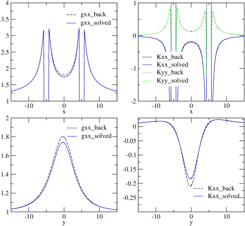
Figure 1: Comparison of background Kerr-Schild superposition data (dashed lines) with the final output of our elliptic constraint equation solver (solid lines). We see that the background is quite close to the physical solution. These particular data were generated for two holes located at $x=\pm 5m$, with spins $a_{1}=a_{2}=0.5$, with the spin of the $x=-5m$ hole tipped by rotation about the $x$ axis by $\theta_{1}=7\pi/8$, and an excision radius of $0.75m$.

4 Generating the physical spacetime

We will consider in this paper physical applications which use superposed Kerr-Schild backgrounds. When multiple black holes are present, the background superposed Kerr-Schild data described in the previous section are not solutions of the constraints, Eqs. (2)–(3). Hence they do not constitute a physically consistent data set. A physical spacetime can be constructed by modifying the background fields with new functions such that the constraints are satisfied. We adopt the conformal transverse-traceless method of York and collaborators YP which consists of a conformal decomposition and a vector potential that adjusts the longitudinal components of the extrinsic curvature. The constraint equations are then solved for these new quantities such that the complete solution fully satisfies the constraints. We do not consider ${\rm tr}K=0$, nor conformally flat, solutions.

The physical metric, $g_{ij}$, and the trace-free part of the extrinsic curvature, $A_{ij}$, are related to the background fields through a conformal factor

$$g_{ij} = \phi^{4}\tilde{g}_{ij},$$ (18)

$$A^{ij} = \phi^{-10}(\tilde{A}^{ij}+\tilde{(lw)}^{ij}),$$ (19)

where $\phi$ is the conformal factor, and $\tilde{(lw)}^{ij}$ will be used to cancel any possible longitudinal contribution to the superposed background extrinsic curvature. $w^{i}$ is a vector potential, and

$$\tilde{(lw)}^{ij}\equiv\tilde{\nabla}^{i}w^{j}+\tilde{\nabla}^{j}w^{i}-\frac{2}{3}\tilde{g}^{ij}\tilde{\nabla_{k}}w^{k}.$$ (20)

The trace $K$ is taken to be a given function

$$K=\tilde{K}.$$ (21)

Writing the Hamiltonian and momentum constraint equations in terms of the quantities in Eqs. (18)–(21), we obtain four coupled elliptic equations for the fields $\phi$ and $w^{i}$ YP :

$$\tilde{\nabla}^{2}\phi = (1/8)\big{(}\tilde{R}\phi+\frac{2}{3}\tilde{K}^{2}\phi^{5}-$$ (22)

$$\phi^{-7}(\tilde{A}{{}^{ij}}+(\tilde{lw})^{ij})(\tilde{A}_{ij}+(\tilde{lw})_{ij})\big{)},$$

$$\tilde{\nabla}_{j}(\tilde{lw})^{ij} = \frac{2}{3}\tilde{g}^{ij}\phi^{6}\tilde{\nabla}_{j}K-\tilde{\nabla}_{j}\tilde{A}{{}^{ij}}.$$ (23)

Our outer boundary condition for $\phi$, namely

$$\partial_{\rho}\left(\rho(\phi-1)\right)|_{\rho\rightarrow\infty}=0.$$ (24)

enforces $\phi\rightarrow 1$ at $\infty$, but does not specify the size (or sign) of the $\rho^{-1}$ term in $\phi$. (Here $\rho^{2}=x^{2}+y^{2}+z^{2}$.) We also take as boundary conditions for the vector $w^{i}$:

$$\partial_{\rho}(\rho w^{i}n_{i})=0,$$ (25)

$$\partial_{\rho}\left(\rho^{2}w^{i}(\delta_{ij}-n_{i}n_{j})\right)=0\,,$$ (26)

where $n_{i}$ is the outward pointing unit spatial normal. Condition (24) is a Robin condition commonly used for computational conformal factor determination. Conditions (25) and (26) were derived by Bonning et al.Bonning .

5 Numerical Methods

We first discuss the computational code and tests, and some code limitations.

The constraint equations Eq. (22), Eq. (23) are solved with a multigrid solver Hawley+Matzner . The present code is essentially the same as that described in Hawley+Matzner , except that it has been extended to the full set of constraint equations, non-flat backgrounds, and features parallel processing. The multigrid scheme is essentially a clever means of eliminating successive wavelength-components of the error via the use of relaxation at multiple spatial scales. It makes use of some sort of local averaging procedure (e.g. Gauss-Seidel relaxation). Such relaxation is extremely effective at eliminating short-wavelength components of the error, or in other words, at “smoothing” the error (i.e., the residual, see below). However, relaxation fails to operate efficiently on long-wavelength components of the error (components that involve discretization points more than a few away from the point at which the solution is sought). Multigrid addresses the solution repeatedly on grids of different discretization, achieving the same efficiency at smoothing every scale.

Because the implementation in the method is also in Hawley+Matzner , we do not repeat it here.

6 Multigrid with Excised regions

In our formulation, the black holes are represented by excised regions. Because we work in Cartesian coordinates, and because we want completely general implementation, we do not typically expect that the excision will be defined by overlapping points on the various grids of different resolution.

Our definition of the excision region is that on each grid, the inner boundary consists of points that lie just inside, i.e. up to one grid point inside, the analytic location of the inner boundary, as shown in Figure 2. While there are exceptional configurations such as cubic excision defined so that the excision boundary lies on points of the coarsest grid, this definition means that generically the size of the excision is larger on the finer grids.

This definition of the inner boundary affects the way in which data are restricted from fine grids to coarse grids. Away from the inner boundary, weighted restriction is performed, as shown in left pane of Figure 3. However, if any of the points used in the weighted average lie on an inner boundary, then these points are not used and instead a simple “copy” operation is performed as shown in the right pane of Figure 3. The inner boundary points themselves may need to be filled in on coarse grids (since on the fine grid they may be excised), and to do this we apply a weighted “inward extrapolation” using a parabolic fit to surrounding fine grid points.

Figure 2: Example of how the inner boundary is defined, showing points on a coarse grid and a fine grid. Inner boundary points are those points which are immediately interior to a circle of radius $r_{\rm ex}$. The large filled circles show normal interior grid points (i.e., non-excised, non-boundary points) on the coarse grid, and the large open circles show boundary points on the coarse grid. The small filled and open circles show fine grid interior points and boundary points, respectively. The small dots show excised points on the fine and/or coarse grids, as appropriate. (Only one quadrant of a full domain is shown in this picture for purposes of clarity.)

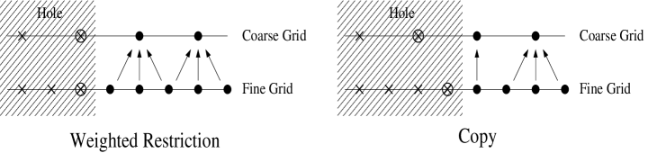
Figure 3: 1-D schematic of scheme for restriction scheme near inner boundary. The circles on the rightmost X’s indicate that this is where the Dirichlet conditions are applied, i.e., there are data on these points. One could use these points in weighted restriction even in the case shown in the right panel. However, we choose never to use these boundary data in weighted restriction, and instead do a simple “copy” operation. The boundary points themselves are updated using either a direct copy, or for coarse grid points over excised fine grid points via an average over parabolic fits of fine-grid data in all available directions.

This scheme has been implemented in a parallel computing environment, using MPI to communicate between processors. Each processor handles a part (a patch) of the total domain. The patch is also logically surrounded by “ghost zones”. Because we deal with a finite-difference representation of derivatives, the communication between processors requires the filling of these “ghost zones” on the borders of the patches, using values computed on other processors, so that derivatives can be accurately computed near the boundaries of the patches. This has implications for the way that smoothing is handled in our simulation.

On a single processor Gauss-Seidel smoothing proceeds across the grid, and the updates at any particular point involve some surrounding points that have been updated and some that have not been. If the same scheme has been implemented on two processors (say splitting the $x-$axis), the buffer region of one patch will already have been updated when the smoother of the other patch begins to use the equivalent points. The order and direction of the filling of the ghost zones can lead to inconsistent behavior (i.e., the result will be different from the single processor result). One solution to this is to insert “wait” commands into the parallel code, so that processors wait to carry out the process in the correct order. This has the effect of slowing the execution, and loses the advantage of parallel processing. A better approach is to use something like red-black Gauss-Seidel. (In 2-d the red-black pattern is like that on a checkerboard.) If the differential operator involves only diagonal second derivatives (no mixed partials) then each point is updated using only points of the opposite color. Then all the reds can be updated before any of the blacks, and vice versa. This ameliorates the ghost zone synchronization problem; the ghost zones can be maintained in the correct state for every step. In this case parallelization works as anticipated.

If the background is taken as flat space, then these conditions apply. But we work with Kerr-Schild forms of the metric which guarantee that there will be mixed partial derivatives in the operators, and the parallel synchronization problem reappears.

Our solution is to introduce what we call rainbow smoothing, in which we make a total of eight passes (like the two passes in red-black smoothing) over the grid, where each pass has a stride width of two over each of the three dimensions of the grid.

7 Verification of constraint Solution

To verify the solution of the discrete equations, we have examined the code’s convergence in some detail. We use a set of completely independent “residual evaluators” for the full Einstein system (here applied only to the initial data), originally constructed by Anderson mattDiss . These evaluate the Einstein tensor, working just from the metric produced by the computational solution, to return fourth order accurate results. They are completely different from the way the equations are expressed in the constraint solver code.

Figure 4 shows such a plot of convergence for the Hamiltonian constraint in an equal mass binary black hole spacetime. The holes are located at $\pm 5m$ on the $x$-axis, where $m$ is the mass of one hole. The elliptic equations were then solved on grids of sizes $385^{3},$ $449^{3},$ and $513^{3},$ giving finest-grid resolutions of approximately $m/12.8$, $m/15$, and $m/17$. We use a five-level multigrid hierarchy. Figure 4 demonstrates almost perfect second order convergence, except near the outer boundary, where the convergence is apparently first order. The second order convergence shows that we have achieved a correct finite difference solution to the initial data problem.

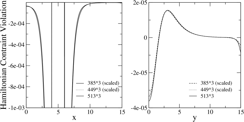
Figure 4: Convergence of the Hamiltonian constraint along the positive $x$ and $y$ axes. We show values of the constraint obtained and three different finest-grid resolutions, $385^{3}$, $449^{3}$ and $513^{3}$, scaled by appropriate ratios of the mesh spacings consistent with second-order convergence. We see that there is good convergence everywhere except near the outer boundaries. Because of this loss of convergence near the outer boundaries, we evaluate the ADM mass over the surface a cube with half-width 12M. (In the left pane, the vertical scale has been exaggerated in order to zoom in on the “body” of the domain, and cuts out the peaks immediately adjacent to the excision regions.

8 Computational Limitations on grid coarseness in excised black hole spacetimes

In the examples given here, where we work on a fixed spatial domain (say $\pm 15m$), the finest resolutions of $385^{3}$, $449^{3}$, $513^{3}$, used in the convergence test correspond to coarsest-grid resolutions of $25^{3}$, $29^{3}$, $33^{3}$, respectively. For the $33^{3}$ grid, the $\pm 15m$ domain is discretized at about $1m$ resolution.

The problem of required resolution for black hole simulations has been discussed in this context at least since the early Grand ChallengeBBHGC efforts. Present computational resources allow much larger grid size than in the Grand Challenge epoch, so the conflict appears at higher resolutions and larger physical domains than previously, and we can do substantial physics with the present configuration. Our approach will be to introduce a multiresolution scheme to maintain required resolution near the central “action”, and allow coarsening further away. To accomplish this we are investigating a mesh-refined multigrid, similar to that described by Brown and Lowebrown . However, for the present work, we simply use very high resolution, the highest that we can presently achieve on the computers available to us, namely $513^{3}$ points using 32 processors.

9 Spin-Spin Effects in Black Hole Interaction

Wald WaldPRD directly computes the force for stationary sources with arbitrarily oriented spins. He considered a small black hole as a perturbation in the field of a large hole. The result found for the spin-spin contribution to the binding energy is

$${E_{b}}=-\left(\frac{\vec{S}\cdot\vec{S^{\prime}}-3(\vec{S}\cdot\hat{n})(\vec{S^{\prime}}\cdot\hat{n})}{d\,^{3}}\right).$$ (27)

Here, $\vec{S}$, $\vec{S}^{\prime}$ are the spin vectors of the sources and $\hat{n}$ is the unit vector connecting the two sources, and $d$ is any reasonable measure of separation that approaches the Euclidean distance $\times(1+{\rm O}(d^{-1}))$ at large $d$ (such as the distance measured in the flat background used in the initial data setting). Dain Dain , using a definition of intrinsic mass that differs from ours (see below), finds binding energy which agrees with Wald’s (Eq. (27)) at ${\rm O}(d^{-3})$.

9.1 Computational Spin-Spin Effects in Black Hole Binding Energy

In order to investigate a computational implementation validating Eq. (27), we begin with a standard definition of the binding energy for black hole interactions.

The total gravitational energy in a binary system can be computed from the initial data using the ADM mass $M_{{\rm ADM}}$, which is evaluated by a distant surface integral (see Eq. (29) below), and gives the Newtonian gravitational mass as measured “at infinity”. For a measure of each hole’s intrinsic mass, we use the horizon mass $M_{\rm AH}$ defined by (Eq. (30)) below. Thus the binding energy, ${E_{b}}$, is defined as

$${E_{b}}=M_{{\rm ADM}}-M_{\rm AH}-M^{\prime}_{\rm AH}.$$ (28)

The ADM mass is evaluated in an asymptotically flat region surrounding the system of interest, and in Cartesian coordinates is given by

$$M_{{\rm ADM}} = \frac{1}{16\pi}\oint\left(\frac{\partial g_{ji}}{\partial x^{j}}-\frac{\partial g_{jj}}{\partial x^{i}}\right){\rm d}S^{i},$$ (29)

The apparent horizon is the only structure available to measure the intrinsic mass of a black hole.‡ Complicating this issue is the intrinsic spin of the black hole; the relation is between horizon area and irreducible mass:

$$A_{\rm H}=16\pi m_{irr}^{2}=8\pi m\left(m+\sqrt{(m^{2}-a^{2})}\right).$$ (30)

As Eq. (30) shows, the irreducible mass is a function of both the mass and the spin, and in general we have no completely unambiguous way specify the spin of the black holes in interaction. But, as was shown in Bonning , the spin evolves only very little until the black holes are very close together. Further, the apparent horizon coincides closely with the event horizon unless the black holes have strong interaction. Hence we assume that the individual spins are correctly given by the spin parameters ${}_{A}a$ specified in forming the superposed Kerr-Schild background, and that the mass is that determined by Eq. (30) using the area determined from the apparent horizon area.

The physical idea in determining the binding energy is that the configuration is assembled from infinitely separated black holes, which are initially on the $x$-axis and which initially have parallel spins. (No energy is required to orient the coordinate system or to adiabatically rotate the spins while the holes are infinitely separated.) Thus these separated holes have their isolated total energy, i.e. $2m$, for equal mass black holes.

Then one of the black holes is adiabatically brought to a particular distance from the other, for instance a coordinate distance of $10m$ as in some of our examples. This is the base configuration from which our computations will start. We then consider the change in the binding energy as we move the direction of the spin axis of one of the black holes.

9.2 ADM angular momentum

Besides the mass, ADM formulae also exist for the momentum $P^{{\rm ADM}}_{k}$ and angular momentum $J^{{\rm ADM}}_{ab}$. These formulæ are also evaluated in an asymptotically flat region surrounding the system of interest Wald ; note4 :

$$P^{{\rm ADM}}_{k} = \frac{1}{8\pi}\oint\left(K_{ki}-K^{b}{}_{b}\delta_{ki}\right){\rm d}S^{i},$$ (31)

$$J^{{\rm ADM}}_{ab} = \frac{1}{8\pi}\oint\left(x_{a}K_{bi}-x_{b}K_{ai}\right){\rm d}S^{i}.$$ (32)

In the data we set, the total momentum is set to zero, so $P^{{\rm ADM}}_{k}=0$. In general, we set data for arbitrarily spinning holes with arbitrary orbital impact parameter, so in general the angular momentum $J^{{\rm ADM}}_{ab}$ is nonzero, and interesting. In the results presented below as code tests, we seek initially non-moving black holes, so the total angular momentum $J^{{\rm ADM}}_{ab}$ is simply the sum of the intrinsic angular momenta, $\Sigma{}_{A}m{}_{a}a$.

9.3 Computational Results

We carried out several series of computational experiments to investigate the spin-spin interaction. In particular we considered instantaneously nonmoving black holes of equal mass $m_{1}=m_{2}=m$, with equal spin parameter $a_{1}=a_{2}=0.5m$. The background separation $d$ for each series was varied from $6m$ to $18m$. For instance, we considered $d=10m$ (holes at coordinate location $x_{1}=-5m$, $x_{2}=5m$). We varied the spin axis of one hole in two different planes, resulting in two “series” of data. The hole at $x=+5m$ (“hole number 2”) was maintained with spin $a_{2}$ aligned with the $z$-axis, while the direction of the other spin $a_{1}$ was varied in a plane in $\pi/8$ steps through $2\pi$ from the $+z$-axis through the $-z$-axis and on back to the $+z$-axis. The difference in the two series is that in one case (the “$yz$ series”) the spin remains in the $y$-$z$ plane; in the other (the “$xz$ series”) it remains in the $x$-$z$ plane. These two configurations are displayed in Figure 5.

Figure 5: The two different BBH configurations investigated. In all cases, the black hole at $x=+d/2$ is held fixed with a constant spin of $a_{2}=0.5$ in the $z$ direction. In the “$xz$ series,” the spin axis of hole at $x=-d/2$ is rotated in the $x$-$z$ plane (i.e. about the $y$ axis) by varying angle $\theta_{1}$ away from the other hole (holding $\varphi_{1}=\pi/2$). In the “yz series,” this axis is rotated in the $y$-$z$ plane by varying $\theta_{1}$ clockwise about the positive $x$ axis. We note that, as an historical artifact of the background generator code of Bonning , angles are defined such that $\varphi=0$ corresponds to the $y$ axis, not the (more typical) $x$ axis.

The domains we used were typically $\pm 15m$, using $513^{3}$ grid points, and typically excising a region of size $r_{ex}=0.9m$. The ADM mass was evaluated on a cube with sides at $\pm 12m$ (i.e., well inside “convergence region” shown in Figure 4 ). (Variations in domain size, resolution, and excision region size were conducted to estimate the dependence of the resulting binding energy on these physically irrelevant but computationally important parameters. For example we conducted a series of runs with outer boundaries at $\pm 20m$ with $513^{3}$ points, evaluating the ADM mass at $\pm 17m$.) The apparent horizon areas were determined using Thornburg’s horizon finder ThornburgAHFinder in the Cactus cactus-grid ; cactus-tools ; cactus-review ; cactus-webpages ; Goodale02a computational toolkit, via a post-processing run on our output files.

As shown in Figures 6 and 7 below, the angular dependence for the binding energy behavior in the $yz$ case is close to that predicted by Wald (Eq. (27)).

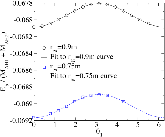
Figure 6: (Normalized) Binding energy vs. spin angle for the $yz$ series. Present in the graph are two curves corresponding to different excision radii $r_{ex}$. For instance a least-squares fit to the $r_{ex}=0.9m$ curve is ${E_{b}/(M_{AH1}+M_{AH2})}=-0.06794-1.396\times 10^{-4}\cos\theta$. For the $r_{ex}=0.75m$ curve, the amplitude of the cosine is $1.381\times 10^{-4}$. This cosine corresponds to the $\vec{S}\cdot\vec{S^{\prime}}$ term in (27). We note that changing the excision radius changes the overall constant offset of the binding energy, but does not have a large effect on the amplitude of the spin-spin interaction.

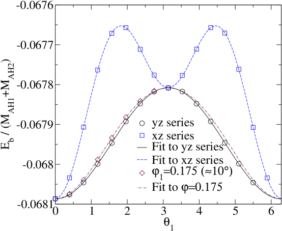
Figure 7: (Normalized) Binding energy vs. spin angle for the $xz$ series (“$\varphi_{1}=\pi/2$”), along with the $r_{ex}=0.9m$ curve from Figure 6 shown for comparison. Also included is a least-squares fit to the $xz$ series: ${E_{b}/(M_{AH1}+M_{AH2})}=-0.0679-1.390\times 10^{-4}\cos\theta-2.762\times 10^{-4}\sin^{2}\theta$. Note that the coefficient of the $\sin^{2}\theta$ term is roughly twice that of those $\cos\theta$ terms both in this graph an Figure 6. Rather than this near factor of 2 we find numerically, considerations based on the mass quadrupole moment would suggest a factor closer to $3/2$, as indicated by (34).

Figure 6 contains two tests of the $yz$ series, computed identically except for a change in the excision radius. We see that the spin dependence of the binding energy is unchanged, but there is an offset in the average binding energy. This binding energy offset ($0.001m$ out of $-0.07m$) is a well known – but small – dependence on the inner boundary condition in the computation of initial data sets for binary black hole systems (see, e.g. Pfeiffer2 , Bonning ). It implies an accuracy in the binding energy (estimated from the value of the offset) of less than $2\%$ of the total binding energy. On the other hand, the behavior of the spin-dependence, the cosine curve in the binding energy, implies a precision much smaller than the peak-peak amplitude of the cosine curve; we estimate $0.02\%$, one tenth of the peak to peak amplitude.

However, Figure 7 for the $xz$ series (where one of the spins tips away from the other) reminds us that there are additional physical effects in play. The Kerr solution has a quadrupole moment arising nonlinearly from its spin. In terms of Newtonian potential for Kerr:

$$\phi=-\frac{m}{d}-\frac{3}{2d^{3}}ma^{2}\cos^{2}\Theta+...;$$ (33)

the quadrupole term is the $\cos^{2}\Theta$ term, where $\Theta$ is the “viewing” angle at which one hole “sees” the other. Given our configurations in which the spins by default are perpedicular to the line of separation, $\Theta=\pi/2$ when $\theta=0$. Thus in terms of our spin-orientation angle $\theta$ the effect may be written as

$$\phi=-\frac{m}{d}-\frac{3}{2d^{3}}ma^{2}\sin^{2}\theta+...;$$ (34)

Here $d$ is a radial coordinate, defined so that angular dependence begins in the metric only at $O(d^{-3})$KipMoments . Hernandez walterHernandez expands the asymptotic Kerr-Schild form and comes to the same result for the quadrupole moment of the Kerr black hole. The quadrupole $\cos^{2}\Theta$ effect is not evident in the $yz$ series because the hole at $+5m$ is always “looking” at the equator of the hole at $-5m$, i.e. at $\Theta=\pi/2$ so there is zero effect. even as the hole at $-5m$ tilts. However, since the $xz$ series tilts the hole at $x=-5m$ away from hole at $x=+5m$, the fixed hole “sees” different latitudes of the rotated hole in the $xz$ series.

Bonning et al.Bonning showed that Kerr-Schild data correctly predicts the Newtonian binding energy $-mm^{\prime}/{d}$. The total binding in a relativistic calculation is this ${\rm O}(d^{-1})$ term, plus Wald’s ${\rm O}(d^{-3})$ spin- spin interaction, plus the quadruole terms in the potential, plus any possible ${\rm O}(d^{-2})$ contribution to the solution.

Following Wald’s notation then, the complete spin dependence may be written as

$${E_{b}}=-\left(\frac{\vec{S}_{1}\cdot\vec{S}_{2}-3(\vec{S}_{1}\cdot\hat{n})(\vec{S}_{2}\cdot\hat{n})}{d\,^{3}}\right).+{3\over 2d\,^{3}}\left({m_{2}\over m_{1}}[\vec{S}_{1}\cdot\hat{n}]^{2}+{m_{1}\over m_{2}}[\vec{S}_{2}\cdot\hat{n}]^{2}\right).$$ (35)

(Note that, for the configurations considered in this paper, $\vec{S}_{2}\cdot\hat{n}=0$.) Both the Wald spin-spin term and the quadrupole moment term in the expansion of the potential are proportional to $d^{-3}$, though this is correct only near infinity; for close distances (such as $d\approx 10m$ considered here) one expects deviations from nonlinear terms in the results. In fact the angular dependence of these terms is remarkably accurately reproduced. Table 1 shows the first four coefficients in fits to the binding energy; the third and fourth power coefficients are substantially below the cosine and cosine-squared coefficients. The Wald formula would produce an amplitude of $0.5^{2}/10^{3}=2.5\times 10^{-4}$ for our case of equal spins of $a=0.5m$ and separation of $d=10m$; the actual coefficient from the fit (after multiplying by the sum of the horizon masses) is $2.97\times 10^{-4}$. This apparent agreement is somewhat of an accident, however, since the expected dependence of $d^{-3}$ is not present in our data, as we will show below. The term arising from the the quadrupole term (the cosine squared term) suggests a coefficient of $3.75\times 10^{-4}$ ($1.5$ times the expected amplitude of the spin-spin term). Our fit to the experiment (the $xz$ series) produces $5.860\times 10^{-4}$.

The Wald formula, Equation (27), predicts no difference in the cosine term ($A_{1}$ in Table 1) between the $xz$ and $yz$ series. (The ($\vec{S}\cdot\hat{n}$) term in Eq. (27) is zero for all experiments carried out because the black hole on the positive $x$ axis has a fixed spin direction parallel to the $z$ axis.) This is the behavior we find; compare the coefficients $B_{1}$ for $\cos\theta$ in Tables 2 and 3.

$\varphi_{1}$	d	$A_{0}$	$A_{1}$	$A_{2}$	$A_{3}$	$A_{4}$
0 (“$yz$ series”)	10	-0.0679461	-1.3985e-4	-1.07477e-6	3.47174e-7	-1.68858e-7
0.175	10	-0.067933	-1.3891e-4	-1.45311e-5	-1.39774e-6	4.15175e-7
1.57 (“$xz$ series”)	10	-0.0676704	-1.3787e-4	-2.74078e-4	-1.55601e-6	-2.17319e-6

Table 1: Table of coefficients for curve fits of the form ${E_{b}/(M_{AH1}+M_{AH2})}=A_{0}+A_{1}\cos\theta+A_{2}\cos^{2}\theta+A_{3}\cos^{3}\theta+A_{4}\cos^{4}\theta$, for a separation of $10m$. (Here and below, we report several significant digits for the purposes of comparison, however due to variations resulting from excision region size and other effects, one would rightly regard only the first two digits as significant.) This shows that terms higher in order than $\cos^{2}\theta$ do not contribute significantly. Because of this, we do not include powers higher than two in the trigonometric basis functions. Also, given the considerations due to the mass quadrupole moment in Eq. (34), all subsequent curve fits in this paper use the form ${E_{b}/(M_{AH1}+M_{AH2})}=B_{0}+B_{1}\cos(\theta)+B_{2}\sin^{2}\theta$. That is, the second order term will be taken as proportional to $\sin^{2}\theta$, not $\cos^{2}\theta$. This results in an offset of the total binding energy ($A_{0}$).

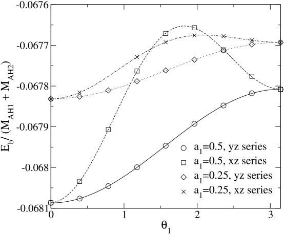
Figure 8: The effects of varying the spin magnitude of one of the holes. Symbols denote data points, lines denote curve fits. Notably, the fit for the $xz$ series with $a_{1}=0.5$ is ${E_{b}/(M_{AH1}+M_{AH2})}=-0.0679464-1.39041\times 10^{-4}\cos\theta+2.76249\times 10^{-4}\sin^{2}\theta$, while for the $xz$ series with $a_{1}=0.25$ it is ${E_{b}/(M_{AH1}+M_{AH2})}=-0.0677621-6.94328\times 10^{-5}\cos\theta+7.00104\times 10^{-5}\sin^{2}\theta$. Thus reducing spin $a_{1}$ from 0.5 to 0.25 results in reduction of the $\cos\theta$ term by a factor of two, while the $\sin^{2}\theta$ term is reduced by nearly a factor of four.

We tested the spin-squared dependence of the $\sin^{2}\theta$ term by two methods. In one we considered $a=a_{1}=0.25m$ for the hole at $x=-5m$, which was then tested in an abbreviated $yz$ series, while $a_{2}$ held at $a_{2}=0.5$ along the positive $z$ axis for the hole at $x=+5m$. Figure 8 shows the result; the effect from the quadrupole term is quadratic in the reduced spin (its amplitude is reduced by a factor of four), while the Wald spin-spin interaction is linear in the reduced spin and its amplitude is reduced by a factor of two. To further test the quadrupole dependence we considered rotating the spin of the black hole at $x=-5m$ in a plane turned by $\varphi_{1}=0.175{\rm rad}\approx 10^{\circ}$. The coefficients of the nonlinear curve fit are listed on the second line of Table 1 and are plotted as interpolating lines in Figure 7. They have the analytically expected dependence.

Series	$d$	$B_{0}$	$B_{1}$	$B_{2}$
$yz$	6	-0.0743885	-0.000381203	4.68096e-6
$yz$	7	-0.0731073	-0.000275675	3.11827e-6
$yz$	8	-0.0716993	-0.000211891	3.06277e-6
$yz$	10	-0.0679473	-0.000139598	1.25165e-6
$yz$	12	-0.0632223	-9.97935e-5	-3.78722e-7
$yz$	14	-0.0576223	-7.85976e-5	-8.578e-8
$yz$	16	-0.0517695	-6.45692e-5	-3.17302e-7
$yz$	18	-0.0459505	-5.52391e-5	-1.16e-6

Table 2: Table of coefficients for curve fits of the form ${E_{b}/(M_{AH1}+M_{AH2})}=B_{0}+B_{1}\cos\theta+B_{2}\sin^{2}\theta$, for the $yz$ series ($\varphi_{1}=0$), for various BBH separations $d$ with both spins $a_{1}=a_{2}=0.5$, using a domain size of $\pm 15m$ and $513^{3}$ fine grid points. Notice that, as expected, $B_{2}$ is very small for all these fits.

Series	$d$	$B_{0}$	$B_{1}$	$B_{2}$
$xz$	6	-0.0743885	-0.000381203	0.000431581
$xz$	7	-0.0731073	-0.000275674	0.000357985
$xz$	8	-0.0716993	-0.00021189	0.000316921
$xz$	10	-0.0679464	-0.000139041	0.000276249
$xz$	12	-0.0632223	-9.97932e-5	0.000224196
$xz$	14	-0.0576223	-7.85974e-5	0.000193869
$xz$	16	-0.0517695	-6.45689e-5	0.000171335
$xz$	18	-0.0459505	-5.52389e-5	0.000146205

Table 3: Table of coefficients for curve fits of the form ${E_{b}/(M_{AH1}+M_{AH2})}=B_{0}+B_{1}\cos\theta+B_{2}\sin^{2}\theta$, for the $xz$ series ($\varphi_{1}=1.57$), for various BBH separations $d$, using a domain size of $\pm 15M$ and $513^{3}$ fine grid points.

Figures 9 and 10 show our tests of the separation-dependence of the binding energy. We expect the constant term $B_{0}$ to fall off asymptotically as $1/d$, since it corresponds to the $M/r$ term in the Newtonian limit. Instead we find roughly linear behavior at the largest separations we are able to compute. The amplitudes $B_{1}$ and $B_{2}$ also fall off differently than expected. We expect both $B_{1}$, which corresponds to the cosine term in (27), and $B_{2}$, which corresponds to the mass quadrupole term, to scale as $d^{-3}$. Instead we find that $B_{1}$ scales as $d^{-2}$, and that $B_{2}$ scales no faster than $d^{-1}$. Since we expect the constant term $B_{0}$ to scale as $1/d$ (although, as in Figure 9, we see that it does not), dividing the amplitudes $B_{1}$ and $B_{2}$ by the constant $B_{0}$ does not significantly illuminate the results. These results for the separation-dependence are likely affected by the outer boundaries of our computational domain in unphysical ways. In the future we hope to repeat these studies with higher resolution and larger domains, using a multi-resolution (mesh refinement) version of our code. For the present, we conducted an additional test to measure the effects of the outer boundary, namely we looked for unphysical effects by computing the difference between the ADM mass and the horizon mass for a single black hole as we rotated its spin axis. The variation we found was on the order of $10^{-6}$, which would appear as a horizontal line in Figure 6. While this provides some assurance that our mass determination methods are functioning to some level of expectation, this (single-hole) effect is insufficient to explain the deviation from the expected results in the binary simulations. Future refinements and larger domains will hopefully clarify this issue.

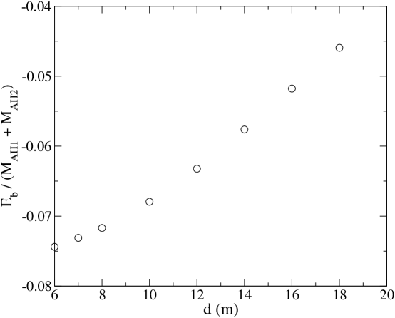
Figure 9: Variation of binding energy vs. BBH separation $d$ (holes at $x=\pm d/2$), showing the constant term $B_{0}$ in the curve fits shown in Table 2. The circles are computed using $513^{3}$ grid points on a domain of $\pm 15m$, evaluating the ADM mass on a cube of half-width $12m$. We note that, at large separations, the curve is roughly linear, in contrast to an expected behavior of $1/d$. We speculate that this (unphysical) effect is due to the outer boundary of the computational domain, in particular the behavior of the ADM mass as estimated at these rather small outer radii. However it may simply be the case that the asymptotic behavior only evident at larger separations. We expect that future work using our multiresolution code with larger domains and higher resolutions should produce better agreement with the expected behavior.

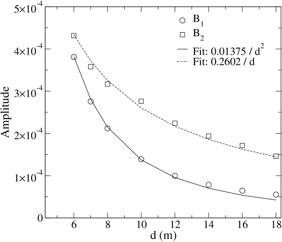
Figure 10: Amplitude vs. separation for the constants $B_{1}$ in Tables 2 and 3 (circles), and $B_{2}$ in Table 3 (squares). Rather than seeing the expected asymptotic $d^{-3}$ fall-off for each amplitude, we find the cosine term $B_{1}$ has roughly $d^{-2}$ behavior, whereas the $\sin^{2}$ term $B_{2}$ falls off no faster than $1/d$.

10 Discussion

To the extent checked, our computational tests of the spin-spin interaction in the binding energy of binary black hole configurations, verify the angular dependence given by Equation (27) WaldPRD . We verified the behavior given by Wald’s $-(\vec{S}\cdot\vec{S}^{\prime})$ term, but since we always kept one black hole’s spin axis perpendicular to the separation axis, we made no attempt to observe the $\vec{S}\cdot\hat{n}$ term in Wald’s formula. At the separations and domains available, our results did not show asymptotic $d^{-3}$ fall-off with distance.

Additionally, we find an effect due to the mass quadrupole moment of the black holes. This results in a higher-order (sine squared) variation with spin angle than given in Wald’s formula. Thus we combine these two effects into a general equation (35) for spin-spin interactions of binary black holes. However, in this case as well, the expected asymptotic fall off of $d^{-3}$ was not evident in our solutions. Future analysis will use a new multiresolution version of our code to further pursue questions raised by the results here, including moving to significantly larger separations to evaluate the asymptotic behavior of the spin-dependent interactions, and effects due to rotation of both holes’ spin axes. We also intend to investigate the spin-orbit coupling and its bearing on evolutions such as Brownsville2 . We are now beginning exploration of the constrained evolution approach in spacetimes involving single moving, and multiple interacting black holes. We find substantial improvement from constraint solving in every simulation.

References

- (1) J. York and T. Piran “The Initial Value Problem and Beyond”, Spacetime and Geometry: The Alfred Schild Lectures, R. Matzner and L. Shepley Eds. University of Texas Press, Austin, Texas. (1982); G. Cook, “Initial Data for the Two-Body Problem of General Relativity”, Ph.D. Dissertation, The University of North Carolina at Chapel Hill (1990).
- (2) N. Ó. Murchadha and J. W. York, Jr., Phys. Rev. D10, 428 (1974); N. Ó. Murchadha and J. W. York, Jr., Phys. Rev. D10, 437 (1974); N. Ó. Murchadha and J. W. York, Jr., Gen. Relativ. Gravit. 7 257 (1976).
- (3) J. W. York, Jr., Phys. Rev. Lett. 82, 1350 (1999).
- (4) J. R. Wilson and G. J. Mathews, Phys. Rev. Lett. 75, 4161 (1995); J. R. Wilson and G. J. Mathews, and P. Marronetti, Phys. Rev. D54, 1317 (1996)
- (5) J. Bowen and J. W. York, Phys. Rev. D21, 2047 (1980).
- (6) R. Wald, Phys. Rev. D6, 406 (1972).
- (7) Y. Choquet-Bruhat, Global Solutions of the Problem of Constraints on a Closed Manifold, Symp. Math.XII 317 (1973).
- (8) A. Lichnerowicz, “L’Integration des Equations de la Gravitation Relativiste et le Probleme des n Corps, J. Math. Pures et Appl. 23 37-63 (1944).
- (9) Scott H. Hawley and Richard A. Matzner Class. Quant. Grav. 21 805-822 (2004).
- (10) R. Arnowitt, S. Deser, and C. Misner in Witten, Gravitation, an Introduction to Current Research (Wiley, New York 1962).
- (11) G. B. Cook, Phys. Rev. D50, 5025 (1994).
- (12) H. P. Pfeiffer, S. A. Teukolsky and G. B. Cook Phys. Rev. D62, 104018 (2000).
- (13) T. Baumgarte Phys. Rev. D62, 024018 (2000).
- (14) E. Gourgoulhon, P. Grandclement and S. Bonazzola, Phys. Rev. D65, 044020 (2002).
- (15) P. Grandclement, E. Gourgoulhon and S. Bonazzola, Phys. Rev. D65, 044021 (2002), and references therein.
- (16) E. Gourgoulhon, P. Grandclement and S. Bonazzola, Int. J. Mod. Phys. A17 2689–94 (2002).
- (17) G. B. Cook Phys. Rev. D65 084003 (2002).
- (18) H. P. Pfeiffer, G. B. Cook, and S. A. Teukolsky Phys. Rev. D66 024047 (2002).
- (19) G. B. Cook, Living Rev. Rel. 3, 5 (2000).
- (20) D. Shoemaker, M. F. Huq and R. A. Matzner Phys. Rev. D62, 124005 (2000).
- (21) M. F. Huq, M. Choptuik and R. A. Matzner, Phys. Rev. D66, 084024 (2002). [arXiv:gr-qc/0002076].
- (22) R. Kerr and A. Schild, “Some Algebraically Degenerate Solutions of Einstein’s Gravitational Field Equations,” in Applications of Nonlinear Partial Differential Equations in Mathematical Physics, Proc. of Symposia B Applied Math., Vol XVII (1965); “A New Class of Solutions of the Einstein Field Equations”, Atti del Congresso Sulla Relitivita Generale: Problemi Dell’Energia E Onde Gravitazionala G. Barbera, Ed. (1965).
- (23) M. Campanelli, C. O. Lousto, P. Marronetti, Y. Zlochower, gr-qc/0511048 (2005).
- (24) J. G. Baker, J. Centrella, D.-I. Choi, M. Koppitz, J. van Meter, gr-qc/0511103 (2005).
- (25) R. Matzner, M. F. Huq and D. Shoemaker, Phys. Rev. D59, 024015 (1999)[arXiv:gr-qc/9805023].
- (26) Erin Bonning, Pedro Marronetti, David Neilsen and Richard Matzner Phys. Rev. D68 (2003) 044019.
- (27) Choptuik M W 1999 Lecture notes, Taller de Verano 1999 de FENOMEC: Numerical Analysis with applications in Theoretical Physics.
- (28) The Binary Black Hole Grand Challenge Alliance: G. B. Cook, M. F. Huq, S. A. Klasky, M. A. Scheel, A. M. Abrahams, A. Anderson, P. Anninos, T. W. Baumgarte, N. T. Bishop, S. R. Brandt, J. C. Browne, K. Camarda, M. W. Choptuik, C. R. Evans, L. S. Finn, G. C. Fox, R. Gomez, T. Haupt, L. E. Kidder, P. Laguna, W. Landry, L. Lehner, J. Lenaghan, R. L. Marsa, J. Masso, R. A. Matzner, S. Mitra, P. Papadopoulos, M. Parashar, L. Rezzolla, M. E. Rupright, F. Saied, P. E. Saylor, E. Seidel, S. L. Shapiro, D. Shoemaker, L. Smarr, W. M. Suen, B. Szilagyi, S. A. Teukolsky, M. H. P. M. van Putten, P. Walker, J. Winicour, J. W. York Jr., “Boosted three-dimensional black-hole evolutions with singularity excision”, Phys. Rev. Lett. 80 2512-2516 (1998) [gr-qc/9711078].
- (29) J. David Brown, Lisa L. Lowe, “Multigrid elliptic equation solver with adaptive mesh refinement”, J. Comput. Phys. 209 582-598 (2005) [gr-qc/0411112].
- (30) K. S. Thorne, “Multipole expansions of gravitational radiation” Rev Mod Phys 52 299 (1980).
- (31) Walter C. Hernandez, “Material Sources for the Kerr Metric”, Phys Rev 159 1070 (1967)
- (32) C. W. Misner, K. S. Thorne, and J. A. Wheeler, Gravitation (W.H. Freeman, New York, 1970).
- (33) R. Wald, General Relativity (University of Chicago Press, Chicago, 1984).
- (34) P. Marronetti, M. Huq, P. Laguna, L. Lehner, R. Matzner and D. Shoemaker, Phys. Rev. D62, 024017 (2000) [gr-qc/0001077].
- (35) P. Marronetti and R. A. Matzner Phys. Rev. Lett. 85 5500 (2000).
- (36) S. Dain Phys. Rev.D66 084019 (2002).
- (37) For consistency of notation we use the superscript “ADM” to decorate the angular momentum . We are not certain where the formula (32) was first written. It does not appear in ADM . Expressions equivalent to it appear in Weinberg and in MTW , and were promulgated in notes by Misner (unpublished) in the mid-60s, arising from the long history of conservation law/pseudo-tensor studies in General Relativity. The form here was taken from Wald ; see also the very thorough development in Brown .
- (38) S. Weinberg, Gravitation and Cosmology (Wiley and Sons, New York, 1972)
- (39) J. D. Brown and J. W. York, Phys. Rev. D47, 1407 (1993).
- (40) D. Brill and R. W. Lindquist Phys. Rev. 131 471 (1963).
- (41) Misner, C. W., “The Method of Images in Geometrostatics”, Ann. Phys. (N. Y.), 24, 102, (1963).
- (42) This was apparently first noticed as a computational result; see A. Čadež, Ann. Phys. (NY) 83 449 (1974). Čadež considered both the Brill-Lindquist Brill and Misner Misner data. For Brill-Lindquist data the apparent horizon areas are easy to compute to , because the lowest order effect of the distant hole on the local one is a constant, isotropic addition to the local value of the conformal factor.
- (43) W. H. Press, S. A. Teukolsky, W. T. Vetterling, and B. P. Flannery, Numerical Recipies in Fortran, Second Edition (Cambridge University Press, Cambridge, 1992).
- (44) H. Pfeiffer L. Kidder, M. Scheel and S. A. Teukolsky, Comput. Phys. Commun. 152 253 (2003).
- (45) P. Brady, J. Creighton and K. S. Thorne, Phys. Rev. D58, 061501 (1998).
- (46) S. Klasky, PhD Dissertation, University of Texas at Austin, (1994).
- (47) Mijan F. Huq, Matthew W. Choptuik and Richard A. Matzner, “Locating boosted Kerr and Schwarzschild apparent horizons,” Phys. Rev. D66, 084024 (2002).
- (48) S. Bonazzola, E. Gourgoulhon, P. Grandclément and J. Novak, “A constrained scheme for Einstein equations based on Dirac gauge and spherical coordinates,” Phys. Rev. D70, 104007 (2004) .
- (49) G. Toth “The B constraint in shock-capturing magnetohydrodynamics codes,” Jour. Comp. Phys. 161, 605 (2002).
- (50) Michael Holst, Lee Lindblom, Robert Owen, Harald P. Pfeiffer, Mark A. Scheel and Lawrence E. Kidder, “Optimal constraint projection for hyperbolic evolution systems,” gr-qc/0407011 (2004).
- (51) Matthew Anderson, “Constrained evolution in numerical relativity,” Ph.D. dissertation, The University of Texas at Austin (2004).
- (52) J. Thornburg, “A Fast Apparent-Horizon Finder for 3-Dimensional Cartesian Grids in Numerical Relativity,” Class. Quant. Grav. 21 743-766 (2004).
- (53) G. Allen, W. Benger, T. Dramlitsch, T. Goodale, H.-C. Hege, G. Lanfermann, A. Merzky, T. Radke, and E. Seidel, in Euro-Par 2001: Parallel Processing, Proceedings of the 7th International Euro-Par Conference, edited by R. Sakellariou, J. Keane, J. Gurd, and L. Freeman (Springer, 2001).
- (54) G. Allen, W. Benger, T. Goodale, H.-C. Hege, G. Lanfermann, A. Merzky, T. Radke, E. Seidel, and J. Shalf, Cluster Computing 4, 179 (2001).
- (55) B. Talbot, S. Zhou, and G. Higgins (2000), http://sdcd.gsfc.nasa.gov/ESS/esmf tasc/Files/Cactus b.html.
- (56) The Cactus Team, The Cactus computational toolkit, http://www.cactuscode.org.
- (57) T. Goodale, G. Allen, G. Lanfermann, J. Mass o, T. Radke, E. Seidel, and J. Shalf, in Vector and Parallel Processing VECPAR2002, 5th International Conference, Lecture Notes in Computer Science Springer, Berlin (2002).
- (58) M. Campanelli, C. O. Lousto, P. Marronetti, Y. Zlochower, gr-qc/0604012 (2006).