The Hyperfine Einstein-Infeld-Hoffmann Potential

Abstract

We use recently developed effective field theory techniques to calculate the third order post-Newtonian correction to the spin-spin potential between two spinning objects. This correction represents the first contribution to the spin-spin interaction due to the non-linear nature of general relativity and will play an important role in forthcoming gravity wave experiments.

The problem of motion in general relativity has shed its seeming academic nature due to pending gravity wave experiments. Both LIGO ligo and LISA LISA expect to detect radiation from inspiralling binaries, and thus building templates for these events has become increasingly important. While for late stages of the inspirals numerical techniques are needed, for the early stages one may calculate in the Post-Newtonian approximation (PN) for small velocities. In relativistic cases one may also calculate analytically when deviations from the Schwarzschild geometry are small. A complicating factor in the building of these templates is the fact that there are multiple scales involved. In particular, the finite size of the object, leads to tidal deformations and dissipation which can then in turn affect potentials as well as radiation. These effects make an exact analytical solution intractable. One might hope that systematically expanding around the point particle approximation would lead to a controlled calculational scheme. This is in fact what one can do by using techniques developed for effective field theories nrgr1 ; nrgr2 ; TASI . While these theories are typically applied to quantum field theories involving multiple scales, we will be applying them here to a purely classical problem. The classical problem shares many of the same calculational hurdles as the quantum problem. In particular, because we are expanding around the point particle approximation, the calculation of potentials, as well as the radiated power loss, entails regularizing divergences. However, since in the EFT we work at the level of the action, these divergences are simply renormalizednrgr1 , and for certain higher dimensional terms in the action lead to a classical renormalization group trajectorygoldbergerwise . The EFT also allows one to power count in a very natural way. Each term in the action has a definite scaling in the expansion parameter and thus we may determine the size of a given effect simply by reading off the scaling of the relevant terms in the action.

In the last few years the 3PN ($(O(v^{6})$) potentials for non-spinning objects have been computed blanchet , but the case of spinning bodies has not reached that level of accuracy. The 2.5PN spin-orbit potential was calculated in owen within a point particle approximation and Hadamard regularization. The leading order spin potentials were obtained in BH , but the spin-spin piece has yet to be computed to 3PN. By using the techniques developed in nrgr1 we may avoid any of the pitfalls of the point particle approximation and tame divergences as well as finite size effects. Following the literature, in the spinning case when we use the term 3PN, we mean order $v^{6}v_{rot}^{2}$, where $v_{rot}$ is the rotational velocity which is taken to be order one, in the “maximally rotating case” and $\epsilon v$ in the “co-rotating case”, where $\epsilon\equiv R/r$ ($\sim v^{2}$ for compact objects), and $R,r$ are the radius of the object and orbit respectively.

In this letter we will be applying these EFT ideas, extended to spinning particles in nrgr3 , to calculate the first-nonlinear correction to the spin-spin potential for compact binaries which arises at 3PN . This correction is the “hyper-fine” analog of the Einstein-Infeld-Hoffmann potential calculated more than seventy years ago EIH . While the high order of this contribution makes it appear to be of only academic interest, such accuracy may indeed be necessary for successful matching v6rational due to the fact that inspirals are tracked over long periods of time.

As explained in nrgr1 , the EFT approach proceeds in two stages. First one matches the full theory of an extended object interacting with gravity onto a world-line action treating each object in isolation. This action consists of a tower of world-line operators, with the coefficients of higher dimensional operators encapsulating the true finite size nature of the underlying particle. These coefficients can be fixed by a matching procedure as discussed for the case of absorption in nrgr2 . At the order we are working the world line action necessary for our calculation is given by

$$S= - \sum_{a}\int m_{a}ds_{a}+\int\frac{1}{2}S_{a}^{IJ}\Omega^{a}_{IJ}(x_{a})d\lambda_{a}$$ (1)

$$- M_{pl}^{2}\int d^{4}x\left(2\sqrt{g}R+(\partial^{\nu}h_{\mu\nu}-\frac{1}{2}\partial_{\mu}h^{\alpha}_{\alpha})^{2}\right)$$

where $s_{a}$ and $\lambda_{a}$ are the proper length and affine parameters for the $a$’th worldline respectively. The last term is the gauge fixing term, which corresponds to the harmonic gauge used in all our calculations. In nrgr3 , following the classic work of Regge and Hanson regge for a relativistic top in flat space, the spin effects are included in a generally covariant fashion by introducing the vierbein degrees of freedom $e^{\mu}_{I}(\lambda_{a})$ on the worldline, which relate the local co-rotating frame to the global frame. The generalized angular velocity is then given by (for each particle)

$$e^{J\nu}\frac{D}{d\lambda}e^{I}_{\nu}=\Omega^{IJ}$$ (2)

and the spin $S_{IJ}$ is the variable conjugate to $\Omega_{IJ}$. Operators describing finite size effects have been left out as they are subleading corrections to the spin-spin effects we are interested here nrgr1 ; nrgr3 . We will come back to this point later on. The form of the world-line action (1) is fixed by reparametrization invariance, which allows us to freely choose the worldline parameter. A wise choice is thus $\lambda=x^{0}$, which will directly lead us to the effective action in the PN frame. Therefore, throughout this letter $v^{\mu}\equiv(1,v^{j}\equiv\frac{dx^{j}}{dx^{0}})$.

We next match onto a theory of potentials. This is accomplished by first expanding the action around the flat space limit, i.e

$$g_{\mu\nu} = \eta_{\mu\nu}+h_{\mu\nu}$$

$$e^{J}_{\mu} = \Lambda^{J}_{\mu}+\frac{h_{\mu}^{\nu}\Lambda_{\nu}^{J}}{2M_{pl}}-\frac{h_{\mu}^{\rho}h_{\rho\sigma}\Lambda^{\sigma I}}{8M_{pl}^{2}}+...$$ (3)

where $\Lambda$ is the Lorentz transformation that relates the local co-rotating and global frames in the flat space limit.

Using the power counting rules developed in nrgr1 ; nrgr3 we expand each term in powers of the relative velocity such that each term in the action scales homogeneously in $v$. This allows us to calculate potentials to arbitrary order in $v$ by drawing all possible Feynman diagrams involving a fixed set of vertices. Before specifying the action, we must choose a gauge for the spin degrees of freedom as well as the tetrad. A common and convenient choice are the Newton-Wigner coordinates

$$e^{\mu}_{0} = \frac{p^{\mu}}{m}$$

$$mS^{0\mu} = S^{\mu\nu}p_{\nu}\to S^{i0}=\frac{1}{2}v^{j}S^{ij}+O(v^{4}),$$ (4)

in which the position and momenta are treated as canonical variables and the spin obeys the traditional angular momentum algebra regge . These constraints, which are not all linearly independent, eliminate the unphysical degrees of freedom. Results in this gauge can be related to other choices via the appropriate coordinate transformations will .

Given this gauge choice, we expand out the action yielding to the leading order spin graviton coupling

$$L_{2}=\frac{1}{2M_{pl}}S^{ij}h^{0i,j},$$ (5)

which arises from expanding $\Omega$ in terms of the tetrad and using (The Hyperfine Einstein-Infeld-Hoffmann Potential). Given that the spin scale as nrgr3

$$S\propto\frac{m^{2}}{M_{pl^{2}}}v_{rot},$$ (6)

we find that this leading order interaction goes like $v^{2}v_{rot}$. Thus the leading order spin-spin potential follows from the Feynman diagram with two of these leading order interactions and thus will scale as $v^{4}v_{rot}^{2}$. It is given by a one graviton exchange diagram leading to

$$V^{ss}_{2PN}=-\frac{G_{N}}{r^{3}}(\vec{S}_{1}\cdot\vec{S}_{2}-3\frac{\vec{r}\cdot\vec{S}_{1}\vec{r}\cdot\vec{S}_{2}}{r^{2}}),$$ (7)

which agrees with the previously derived results BH . We will use throughout the paper $S^{ij}\equiv\epsilon^{ijk}S^{k}$ (for different definitions see regge ; owen ), and the standard notation labelling the post-Newtonian order by the power of the orbital velocity.

To work to next order we must consider vertices involving spin to order $v^{3}v_{rot}$. At this order we have

$$L_{3}=\frac{1}{2M_{pl}}S^{jk}v^{i}h^{ik,j}+\frac{1}{4M_{pl}}v^{l}S^{jl}h^{00,j}\\$$

while at order $v^{4}v_{rot}$ we must include

$$L_{4} = \frac{1}{4M_{pl}}v^{l}S^{lj}v^{i}h^{i0,j}+\frac{1}{4M_{pl}}v^{l}S^{lj}h^{0j,0}.$$

These terms arise by keeping higher order pieces in the spin matrix (i.e. $S_{0i}$) as well as time derivatives which are down by $v$ relative to spatial derivatives. Since we are calculating to order $v^{6}v_{rot}^{2}$ (3PN) we must include diagrams with one insertion of $L_{4}$ and a leading order vertex $L_{2}$, as well as those diagrams with two insertions of $L_{3}$. These diagrams are depicted in Figures (1a) and (1b). There is a further contribution from one graviton exchange which arises from the first correction to the graviton Green’s function

$$G(p)\propto\frac{1}{p_{0}^{2}-\vec{p}^{2}}\approx-\frac{1}{\vec{p}^{2}}-\frac{p_{0}^{2}}{\vec{p}^{4}}+.~{}.~{}.$$ (8)

which reflects the first deviation from instantaneity in the exchange. This contribution is depicted in Figure (1c) and, more formally, arise from new vertices in the action nrgr1 .

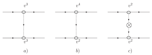
Figure 1: Diagrams contributing to 3PN order which do not involve non-linear interactions. The blow represents a spin insertion and the cross corresponds to a propagator correction.

At order 3PN we must also include diagrams with double graviton exchange (note that we need not include diagrams which can be disconnected by cutting the world-line, as these are iterations of connected diagrams which are automatically resummed when solving the equations of motion). Terms quadratic in the metric arise from the higher order terms in the vierbein and the connection. After expanding we find that the relevant pieces of the Lagrangian are

$$L_{h^{2}}=\frac{1}{4M_{pl}^{2}}S^{ij}(h^{ik}(h^{k0,j}-h^{j0,k})-h^{i0}h^{00,j}).$$ (9)

These terms scale as $v^{4}v_{rot}$ thus, we must include all diagrams for which a leading order spin vertex ($v^{2}v_{rot}$) and a leading order mass insertion from the non-spinning part of the action

$$L_{0}=-\frac{m}{2M_{pl}}h_{00},$$ (10)

are contracted. The resulting diagram is shown in Figure (2b). Finally we must include the contribution from those diagrams including the three graviton vertex which scales as $v^{2}$ nrgr1 . This vertex is too voluminous to include here, and is best, and quite simply, handled using a symbolic manipulation program All such diagrams resulting from this vertex, two leading order spin insertions and one leading order mass insertion must be included (see Figure (2a)).

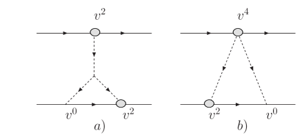
Figure 2: Non-linear contributions to the 3PN spin-spin potential.

Combining all of the contributions leads to the potential

$$V^{ss}_{3PN} = -\frac{G_{N}}{2r^{3}}\left[\vec{S}_{1}\cdot\vec{S}_{2}\left({3\over 2}\vec{v}_{1}\cdot\vec{v}_{2}-3\vec{v}_{1}\cdot{\vec{n}}\vec{v}_{2}\cdot{\vec{n}}-\left(\vec{v}_{1}^{2}+\vec{v}_{2}^{2}\right)\right)-\vec{S}_{1}\cdot\vec{v}_{1}\vec{S}_{2}\cdot\vec{v}_{2}-\frac{3}{2}\vec{S}_{1}\cdot\vec{v}_{2}\vec{S}_{2}\cdot\vec{v}_{1}+\vec{S}_{1}\cdot\vec{v}_{2}\vec{S}_{2}\cdot\vec{v}_{2}\right.$$ (11)

$$+ \vec{S}_{2}\cdot\vec{v}_{1}\vec{S}_{1}\cdot\vec{v}_{1}+3\vec{S}_{1}\cdot\vec{n}\vec{S}_{2}\cdot\vec{n}\left(\vec{v}_{1}\cdot\vec{v}_{2}+5\vec{v}_{1}\cdot\vec{n}\vec{v}_{2}\cdot\vec{n}\right)-3\vec{S}_{1}\cdot\vec{v}_{1}\vec{S}_{2}\cdot\vec{n}\vec{v}_{2}\cdot\vec{n}-3\vec{S}_{2}\cdot\vec{v}_{2}\vec{S}_{1}\cdot\vec{n}\vec{v}_{1}\cdot\vec{n}$$

$$+ \left.3(\vec{v}_{2}\times\vec{S}_{1})\cdot\vec{n}(\vec{v}_{2}\times\vec{S}_{2})\cdot\vec{n}+3(\vec{v}_{1}\times\vec{S}_{1})\cdot\vec{n}(\vec{v}_{1}\times\vec{S}_{2})\cdot\vec{n}-\frac{3}{2}(\vec{v}_{1}\times\vec{S}_{1})\cdot\vec{n}(\vec{v}_{2}\times\vec{S}_{2})\cdot\vec{n}\right.$$

$$- \left.6(\vec{v}_{1}\times\vec{S}_{2})\cdot\vec{n}(\vec{v}_{2}\times\vec{S}_{1})\cdot\vec{n}\right]+\frac{3G^{2}_{N}(m_{1}+m_{2})}{r^{4}}\left(\vec{S}_{1}\cdot\vec{S}_{2}-3\vec{S}_{1}\cdot\vec{n}\vec{S}_{2}\cdot\vec{n}\right),$$

with $\vec{n}\equiv\frac{\vec{r}}{r}$. The equations of motion simply follow from the usual Hamiltonian procedure.

The leading order finite size contribution arise from so-called self induced effects. That is, corrections to sphericity arising from the non-vanishing quadrupole moments induced by rotation. These effects are encapsulated by the world-line operator

$$L_{ES^{2}}\equiv\frac{C}{2mM_{pl}}\frac{E_{\mu\nu}}{\sqrt{u^{2}}}S^{\mu}_{\rho}S^{\rho\nu},$$ (12)

where $C$ is a constant which is determined by the nature of the object and $E_{\mu\nu}$ is the electric component of the Weyl tensor. In the case of a rotating black hole $C=1$, and this term represents the non-vanishing quadrupole moment of the Kerr solution thorne . For neutron stars $C$ ranges between $4$ and $8$ depending on the equation of state of the neutron star matter poisson . This operator scales as $v^{4}v_{rot}^{2}$ at leading order, and it is easy to show that it gives rise to a 2PN (quadrupole-monopole) spin-orbit contribution poisson2 ; nrgr3 ,

$$V^{so}_{2PN}=-\frac{CG_{N}m_{2}}{2m_{1}r^{3}}\left(\vec{S}_{1}\cdot\vec{S_{1}}-3(\vec{n}\cdot\vec{S}_{1})^{2}\right)+\;1\leftrightarrow 2,$$ (13)

so one might then think that it will also contribute at 3PN in the spin-spin sector, since naively one could contract (12) with a leading order spin interaction (5). However, this contribution vanishes, and the leading order finite size effects in the spin-spin potential show up at 3.5PN. There is nevertheless a finite size correction in the spin-orbit interaction at 3PN coming from diagrams where (12) is contracted with subleading mass insertions as well as corrections to instantaneity and non linear effects. We will report on these results in a forthcoming paper.

As discussed in nrgr1 the inclusion of radiation into this formalism is accomplished by working in a background field. In the background field gauge, after multipole expanding the field to keep manifest power counting grinroth , and integrating over (i.e. solving the equations of motion) the potential gravitons, one generates an effective action for the sources and the radiation graviton $\Gamma[x,\dot{x},h]$ which is invariant under small diffeomorphisms. The power loss due to radiation then follows by calculating the imaginary parts of all vacuum diagrams (i.e. no external gravitons), whereas the real part introduces radiation reaction effects into the equations of motion for the sources. Including spin effects in radiation follows in a similarly straightforward manner by simply including vertices in which the spin couples to the background field. We have calculated the effects of spin on radiation to 2PN and find agreement with those in the literature spinrad . These results along with new results for the 3PN contributions to radiation and quasicircular orbits with the inclusion of spin, will follow in a subsequent publication.

Finally, it is hopefully clear that there are no stumbling blocks in going beyond 3PN in our formalism. It is simply a matter of bookkeeping. Since every term in the action scales homogeneously in the velocity this is not a difficult task. One simply draws all possible diagrams such that the net scaling of all the vertices is of the desired accuracy. For instance, at next order one would need the four-graviton vertex as well as the higher order vertices with and without spin and a contact term involving one source and three graviton lines. Divergences are not an issue as they are all absorbed into their appropriate counter-terms. They are irrelevant until one reaches the order at which finite size operators become relevant, at which point renormalization is straightforward.

We thank Scott Hughes, Eric Poisson and Jure Zupan for helpful comments. Work supported by DOE contracts DOE-ER-40682-143 and DEAC02-6CH03000.

References

- (1) See e.g. A. Abramovici et al., Science 256, 325 (1992); A. Giazotto, Nucl. Instrum. Meth. A 289, 518 (1990).
- (2) K. Danzmann, Class. Quant. Grav. 14, 1399 (1997).
- (3) W. Goldberger and I.Z Rothstein, arXiv:hep-th/0409156, to appear in Phys. Rev. D.
- (4) W. D. Goldberger and I. Z. Rothstein, arXiv:hep-th/0511133, to appear in Phys. Rev. D.
- (5) For a pedagogical introduction to EFT’s see I. Z. Rothstein, arXiv:hep-ph/0308266.
- (6) W. D. Goldberger and M. B. Wise, Phys. Rev. D 65, 025011 (2002) [arXiv:hep-th/0104170].
- (7) L. Blanchet, T. Damour, G. Esposito-Farese and B. R. Iyer, Phys.Rev.Lett. 93, 091101 (2004).
- (8) H. Tagoshi and A. Ohashi and B. Owen, Phys. Rev. D 63, 044006 (2001).
- (9) B.M. Barker and R.F. O’Connell, Gen. Relativ. Grav., 11, 149 (1979). K.S. Thorne and J.B. Hartle, Phys. Rev. D 31, 1815 (1985).
- (10) R. A. Porto, arXiv:gr-qc/0511061, to appear in Phys. Rev. D.
- (11) A. Einstein, L. Infeld and B. Hoffmann, Annals Math. 39, 65 (1938).
- (12) See for instance, E. Poisson and C. M. Will, Phys. Rev. D 52, 848 (1995).
- (13) A. Hanson and T. Regge, Ann. Phys. (N.Y.) 87, 498 (1974).
- (14) L. E. Kidder, Phys. Rev. D 52, 821 (1995) C. Will, Phys. Rev. D 71, 084027 (2005) .
- (15) K.S. Thorne, Rev. Mod. Phys. 52, 299 (1980).
- (16) W.G. Laarakkers and E. Poisson, Astrophys. J. 521, 282 (1999).
- (17) E. Poisson, Phys.Rev. D 57, 5287 (1998).
- (18) B. Grinstein and I. Z. Rothstein, Phys. Rev. D 57, 78 (1998) [arXiv:hep-ph/9703298].
- (19) L. E. Kidder, C. M. Will and A. G. Wiseman, Phys. Rev. D 47, 4183 (1993).