Abstract

Homogeneous cosmological solutions are obtained in five dimensional space time assuming equations of state $p=k\rho$ and $p_{1}=\gamma\rho$ where p is the isotropic 3 - pressure and $p_{1}$, that for the fifth dimension. Using different values for the constants k and $\gamma$ many known solutions are rediscovered. Further the current acceleration of the universe has led us to investigate higher dimensional gravity theory, which is able to explain acceleration from a theoretical view point without the need of introducing dark energy by hand. We also extend a recent work of Mohammedi where using a special form of the extra dimensional scale factor a new interpretation of the higher dimensional equations of motion is given and the concept of an effective four dimensional pressure is introduced. Interestingly the 5D matter field remains regular while the effective negative pressure is responsible for the inflation. Relaxing the assumptions of two equations of state we also present a class of solutions which provide early deceleration followed by a late acceleration in a unified manner. Relevant to point out that in this case our cosmology apparently mimics the well known quintessence scenario fuelled by a generalised Chaplygin-type of fluid where a smooth transition from a dust dominated model to a de Sitter like one takes place. Depending on the relative magnitude of the different constants appearing in our solutions we show that some of the cases are amenable to the desirable property of dimensional reduction.

KEYWORDS : cosmology; higher dimensions; accelerating universe
PACS : 04.20, 04.50 +h

1. Introduction

There are growing evidences today that the current expansion of the universe is accelerating. It follows directly from the findings of Ia Supernovae and indirectly from CMBR fluctuations. The latter observation points to the fact that the average mass density of the universe is very close to critical density. But the large scale structure of our universe indicates that normal gravitating ( but invisible ) matter can account for only 30% into the energy budget. One is naturally left with remaining 70% of the energy which is some mysterious agent responsible for the cosmic acceleration. If we put faith in FRW type of models then General Relativity is unambiguous about the need for some sort of dark energy source to explain the acceleration, which should behave like a fluid with a large negative pressure in the form of a time dependent cosmological constant or an evolving scalar field called quintessence. However none of the existing dark energy models is completely satisfactory. Moreover, it is very difficult to construct a theoretical basis for the origin of this exotic matter, which is seen precisely at the current epoch when one needs the source for cosmic acceleration ( coincidence problem ).
So there has been a resurgence of interests among relativists, field theorists, astrophysicists and people doing astroparticle physics both at theoretical and experimental levels to address the problems coming out of the recent extra galactic observations (for a lucid and fairly exhaustive exposition of some of these ideas one is referred to [1] and references therein ) without involving a mysterious form of scalar field by hand but looking for alternative approaches [2],[3] based on sound physical principles.Viswakarma [4] in a series of papers argued that it is possible to explain the recent observational findings in the frame work of a decelerating model also. Another suggestion is that light emitted from a distant supernova encounters an obstacle enroute to us and gets partially absorbed apparently dimming the supernovae [5] due to flavour oscillations. It occurs when there are several degrees of freedom whose interaction eigenstates coincide with the propagation eigenstates. Such particles can turn into other particles and evade detection. Other alternatives include modification of the Einstein- Hilbert action through the introduction of additional curvature terms, $R^{m}+R^{n}$ ( $m>0,n<0$ and not necessarily integer) in the Lagrangian [6],[7]. The effective Friedmann equations contain extra terms coming from higher curvatures which may be viewed as a fluid, responsible for the current acceleration. However the resulting field equations are extremely difficult to solve and moreover, the cosmology is mostly unstable against perturbations. Hence this curvature quintessence has also of late somewhat fallen from grace.
On the other hand , serious attempts are recently being made [8],[9],[10] to incorporate the phenomenon of accelerating universe within the framework of higher dimensional space time itself without involving any mysterious scalar field with large negative pressure by hand. The attempt to unify gravity with other forces in nature is an active field of research. Some earlier works [11],[12] have been directed at studying theories in which the dimensions of space time is greater that the ( 3+1 ) of the world we observe. Moreover, the advance of super gravity in 11D and super string in 10D indicate that the multidimensional space is apparently a fairly adequate reflection of dynamics of interaction over distances $r\ll 10^{-16}$ cm. where unification of all types of forces may occur. Recent spurt in activities also stems from its applications to brane cosmology. The realisation that the universe is currently undergoing an accelerated expansion phase and the quest for the nature of the quintessence field have renewed the interest in higher dimensional gravity and their relation to cosmology. This is due to the fact that the higher dimensional corrections to the Einstein’s field equations can be viewed as an effective fluid and this fluid can emulate the action of the homogeneous part of the quintessence field. Hence, in this extra dimensional quintessence scenario, what we observe as a new component of cosmic energy density is an effect of higher dimensional corrections to the Einstein-Hilbert action. This approach has definite advantage over the standard quintessence scenario because we do not need to search for the quintessence scalar field and pick them by hand. On the contrary the extra fluid responsible for the acceleration is geometrical in origin having strong physical foundation and also in line with the spirit of general relativity as proposed first by Einstein [13] and later developed by Wesson [11]. In a recent communication [14] it is also argued that quantum fluctuations in 4D spacetime do not give rise to dark energy. Rather a possible source of dark energy is the fluctuations in quantum fields , including quantum gravity inhabiting extra compactified dimensions.
Here we have taken a 5D homogeneous line element with a zero curvature spherically symmetric 3D space. The motivation for the present work is primarily twofold. Assuming two equations of state as $p=k\rho$ and $p_{1}=\gamma\rho$ we have solved the field equations and in the process have recovered some of the important earlier works in this field as special cases. On the other hand to conform to the current accelerating phase of the universe we have searched for quintessential behaviour of our solutions, if any. We get the interesting result in sections 2 and 3 that for a realistic 5D matter field characterised by $0<k$, $\gamma<1$ it is impossible to get accelerating universe with a power law solution for the 3D scale factor. This is in line with the 4D cosmology also. We also calculate the limiting values of $k$ and $\gamma$ when the cosmology shows the desirable property of dimensional reduction. Moreover, while working in higher dimensional theories it is not enough to show spontaneous compactification occurs. The cosmological consequences of the shrinking extra dimensions should also be taken into account. In this context we have extended a recent work of Mohammedi[15] who gave an alternative interpretation of additional higher dimensional terms appearing in the field equations to argue that a regular matter field in higher dimension can generate, in principle at least, an effective pressure which may be negative to trigger an inflation of the 4D spacetime. This is dealt with in section 4 where we have put forward a specific solution to illustrate our point. In section 5 we have assumed a specific form of the deceleration parameter to find a solution of the scale factor for shear free expansion. We get a class of solutions with interesting physical properties. An additional free parameter appearing in the expression of the scale factor characterises the form of the matter field similar to the well known form of the generalised Chaplygin gas for quintessential models. The resulting energy momentum tensor behaves like a mixture of cosmological constant and a perfect fluid obeying higher dimensional equation of state. When the cosmological radius is small the matter field in the form of dust( for example) predominates giving a decelerating expansion till the cosmological term takes over effecting a smooth transition to the current accelerating phase, while in the intermediate stage our cosmology interpolates between different phases of the universe. This phenomena has been exhaustively discussed in the context of quintessence in 4D spacetime. However we are not aware models of similar kind in higher dimensional spacetime, that too without assuming by hand any form of an extraneous scalar field with mysterious properties The paper ends with a discussion in section 6.

2. The Field Equations and its integrals

We begin with considering a (d+4)-dimensional line-element

$$ds^{2} = dt^{2}-R^{2}\left(\frac{dr^{2}}{1-Kr^{2}}+r^{2}d\theta^{2}+r^{2}sin^{2}\theta d\phi^{2}\right)-A^{2}\gamma_{ab}dy^{a}dy^{b}$$ (1)

where $y^{a}$( a,b = 4,…. ,3+d) are the extra dimensional coordinates and the 3D and extra dimensional scale factors R and A depend on time only and K is the 3D curvature and the compact manifold is described by the metric $\gamma_{ab}$. For our manifold $M^{1}\times S^{3}\times S^{d}$ the symmetry group of the spatial section is $O(4)\times O(d+1)$. The stress tensor whose form will be dictated by Einstein’s equations must have the same invariance leading to the energy momentum tensor as [16]

$$T_{00}=\rho~{},~{}~{}T_{ij}=-p(t)g_{ij}~{},~{}~{}T_{ab}=-p_{d}(t)g_{ab}$$ (2)

where the rest of the components vanish. Here p is the isotropic 3- pressure and $p_{d}$, that in the extra dimensions. Assuming two equations of state $p=k\rho$ and $p_{d}=\gamma\rho$, we get from the Bianchi identity $T^{AB}_{;A}=0$

$$\dot{\rho}+\left[3\frac{\dot{R}}{R}(1+k)+d\frac{\dot{A}}{A}(1+\gamma)\right]\rho=0$$ (3)

The last equation integrates to

$$\rho=R^{-3(1+k)}A^{-d(1+\gamma)}$$ (4)

Using equation(4) the independent field equations for our metric (1) are

$$\frac{\rho}{2\beta} = \left\{3\frac{\dot{R^{2}}+K}{R^{2}}-\lambda\right\}+\frac{1}{2}d(d-1)\frac{\dot{A^{2}}}{A^{2}}+3d\frac{\dot{R}\dot{A}}{RA}+\frac{d}{2}(d-1)\frac{\kappa}{A^{2}}$$ (5)

$$= R^{-3(1+k)}A^{-d(1+\gamma)}$$

$$\equiv \left\{3\frac{\dot{R^{2}}+K}{R^{2}}-\lambda\right\}+\frac{\rho_{0}}{2\beta}$$

$$\frac{p}{2\beta} = \left\{-2\frac{\ddot{R}}{R}-\frac{\dot{R^{2}}}{R^{2}}-\frac{K}{R^{2}}+\lambda\right\}-d\frac{\ddot{A}}{A}-\frac{1}{2}d(d-1)\frac{\dot{A^{2}}}{A^{2}}-2d\frac{\dot{R}}{R}\frac{\dot{A}}{A}-\frac{d}{2}(d-1)\frac{\kappa}{A^{2}}$$ (6)

$$= kR^{-3(1+k)}A^{-d(1+\gamma)}$$

$$\equiv \left\{-2\frac{\ddot{R}}{R}-\frac{\dot{R^{2}}}{R^{2}}-\frac{K}{R^{2}}+\lambda\right\}+\frac{p_{0}}{2\beta}$$

$$\frac{p_{d}}{2\beta} = -3\frac{\ddot{R}}{R}-3\frac{\dot{R^{2}}}{R^{2}}-3\frac{K}{R^{2}}+\lambda-(d-1)\frac{\ddot{A}}{A}-\frac{1}{2}(d-1)(d-2)\frac{\dot{A^{2}}}{A^{2}}$$ (7)

$$- 3(d-1)\frac{\dot{R}}{R}\frac{\dot{A}}{A}-\frac{1}{2}(d-1)(d-2)\frac{\kappa}{A^{2}}$$

$$= \gamma R^{-3(1+k)}A^{-d(1+\gamma)}$$

where $\lambda$ is a higher dimensional cosmological constant, $\kappa$ is the curvature of the extra space and 2$\beta$ is the $(d+4)$-dim. gravitational coupling constant. In what follows we assume for simplicity a 5D spacetime$(d=1)$ although we believe many of our results can be extended even when $d>1$. However, in section 4 we will have occasion again to discuss the general line element(1). The last three equations are not independent. We take the following two combinations as our key equations to be solved

$$\frac{\ddot{R}}{R}+\frac{(1+3k)}{2}\frac{(\dot{R^{2}}+K)}{R^{2}}+\frac{(2+3k)}{2}\frac{\dot{R}\dot{A}}{RA}+\frac{1}{2}\frac{\ddot{A}}{A}=0\\$$ (8)

and

$$\frac{\ddot{R}}{R}+(1+\gamma)\frac{\dot{R^{2}}+K}{R^{2}}+\gamma\frac{\dot{R}\dot{A}}{RA}=0$$ (9)

At this stage we take for simplicity K = 0, and the equation (9) then yields a first integral as

$$A=\frac{\alpha}{\dot{R^{\frac{1}{\gamma}}}R^{\frac{(1+\gamma)}{\gamma}}}$$ (10)

where $\alpha$ is a constant of integration. For simplicity we take a power law solution for the scale factor

$$R=t^{m}$$ (11)

which gives via equation (10)

$$A=t^{\frac{-(2m+m\gamma-1)}{\gamma}}\\$$ (12)

The equation (8) further restricts the value of m as $m=\frac{1}{2}~{},~{}~{}\frac{1-\gamma}{\gamma^{2}-3k\gamma+2}$. The former value of m gives $R=t^{\frac{1}{2}}$ and $A=t^{-\frac{1}{2}}$ as also $p=p_{5}=\rho=0$. Incidentally this is the wellknown solution of Chodos and Detweiler [17] for a matter free 5D model. The second value of m gives the following solutions as

$$R = t^{\frac{1-\gamma}{\gamma^{2}-3k\gamma+2}}$$ (13)

$$A = t^{\frac{2\gamma-3k+1}{\gamma^{2}-3k\gamma+2}}$$ (14)

$$\rho = \frac{3(1-\gamma)(\gamma-3k+2)}{(\gamma^{2}-3k\gamma+2)^{2}t^{2}}$$ (15)

$$p = k\rho$$ (16)

$$p_{5} = \gamma\rho$$ (17)

3. Dynamical Behaviour

In what follows we shall see that physical considerations put some restrictions on the values of k and $\gamma$. If we believe in an expanding universe $\gamma=1$ is clearly ruled out from equation (13). Further it is evident that the 3- space expands for $0<\gamma<1$ and $0<k<1$. Again $\rho>0$ demands $0<k<\frac{\gamma+2}{3}$. If the cosmic evolution is amenable to the desirable properly of dimensional reduction it further restricts k as $\frac{2\gamma+1}{3}<k<\frac{\gamma+2}{3}$.

Accelerating universe - I

As discussed earlier in the introduction that our universe is presently accelerating and at the early phase it was decelerating . The early deceleration is physically relevant in the sense that it allows structure formation while the present day acceleration is in conformity with the current data from the supernovae. So we now calculate the deceleration parameter for our metric as

$$q=-\frac{\ddot{R}R}{\dot{R^{2}}}=\frac{\gamma^{2}+(1-3k)\gamma+1}{1-\gamma}$$ (18)

It is well known that both $\gamma$ and $k$ should be less than one. But if we consider the condition $0<\gamma<1$, a little algebra shows that for acceleration $k$ must be greater than 1 which is not desirable. So it is concluded that for power law expansion acceleration is not possible for the condition $0<\gamma<1$ and $\frac{2\gamma+1}{3}<k<\frac{\gamma+2}{3}$. Simple calculation shows that acceleration is possible when $-1<\gamma<-2+\sqrt{3}$ and $-1<k<\left(\frac{\gamma^{2}+\gamma+1}{3\gamma}\right)$. But in this case dimensional reduction is not possible. Here three dimensional scale factor expands indefinitely, matter density is positive and acceleration is possible. The above features are shown in the figure 1.

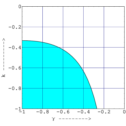
Figure 1: The shaded region corresponds to the range of $\gamma$ and k where universe is accelerating, 3D scale factor is expanding and $\rho$ is positive but no dimensional reduction

If we calculate 4D volume,

$$V=R^{3}A=t^{\frac{-\gamma-3k+4}{\gamma^{2}-3k\gamma+2}}$$ (19)

it is evident that it expands indefinitely. For a particular value of $k$ and $\gamma$, all the features are shown in the figure 2.

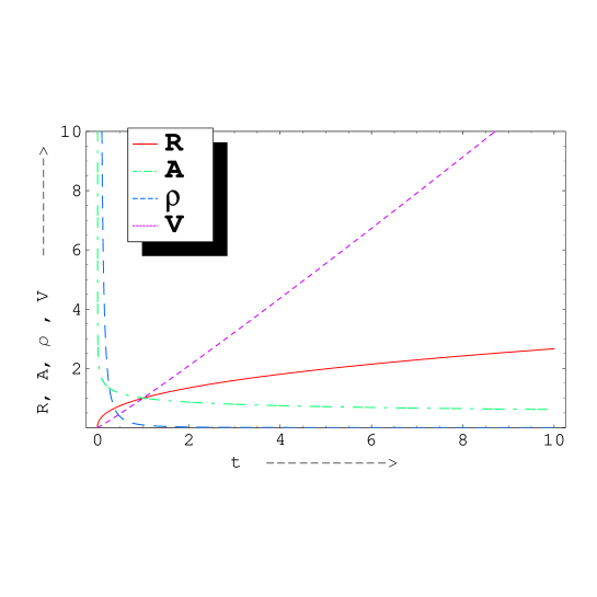
Figure 2: The time evolution of R, A, $\rho$ and V are shown in this figure taking the positive value of $\gamma$ and k

At this stage correspondence to some earlier works in this field may be of interest.

1. As discussed earlier when $m=\frac{1}{2}$,  $\rho=p_{5}=p=0$ and we recover the well known solution of Chodos and Detweiler [17] in vacuum when dimensional reduction takes place.

2. For $k=\gamma=0$, we get the earlier solution of Grøn [18] as

$$R=A=t^{\frac{1}{2}},\\ ~{}~{}p=p_{5}=0,\\ ~{}~{}\rho=\frac{3}{2t^{2}}$$ (20)

where an isotropic expansion in all five dimensions for dust fluid takes place.

3. Next we consider a matter field such that the pressure is isotropic in all dimensions ( $k=\gamma$ )

$$R=A=t^{\frac{1}{2(1+k)}}\\ ,~{}~{}p=p_{5}=\frac{3k}{2t^{2}(1+k)^{2}}\\ ,~{}~{}\rho=\frac{p}{k}$$ (21)

This is the homogeneous case of our earlier work [19].

4. When we consider 3D radiation case, i.e., $k=\frac{1}{3}$, we get the following solutions.

$$R=t^{\frac{(1-\gamma)}{(\gamma^{2}-\gamma+2)}},~{}~{}A=t^{\frac{(2\gamma)}{(\gamma^{2}-\gamma+2)}},~{}~{}p=\frac{(1-\gamma^{2})}{(\gamma^{2}-\gamma+2)^{2}t^{2}},~{}~{}p_{5}=3\gamma p,~{}~{}\rho=3p$$ (22)

for $0<\gamma<1$, three dimensional scale factor expands indefinitely, but dimensional reduction is not possible for extra space. $\rho$ is also positive for this condition. Again for $-1<\gamma<0$ dimensional reduction is possible and $\rho>0$ in this condition. But extra dimensional pressure will be negative. No acceleration is possible here, i.e., $q>0$. R expands indefinitely.

5. For $k=\gamma=-1$ , we can not get the solutions simply by putting these values in the expressions (13-17). The field equations are separately solved for such a case and the solutions are given by

$$R=A=e^{mt},~{}~{}\rho=p=p_{5}=6m^{2}$$ (23)

The above solutions are same as homogeneous case of our earlier work [19]. To sum up, these solutions resemble some special cases of [20], [21]

4. Mohammedi’s work

In a recent communication Mohammedi [15] put forward a new proposal regarding the interpretation of matter field as also of the higher dimensional equations of motion. Closely following his arguments we have in this section presented and discussed a few more results. But before presenting our work proper we would like to very briefly summarise his main results skipping intermediate mathematical details. The cardinal point in Mohammedi’s work is that if one assumes apriori a relationship between the 3D scale factor and the extra scale as

$$\frac{\dot{A}}{A}=-n\frac{\dot{R}}{R}$$ (24)

( n is an arbitrary constant) the FRW equations of standard 4D cosmology are obtained precisely through defining a new term what he calls an effective pressure expressed in terms of the components of the higher dimensional energy momentum tensor. Thus one defines the effective pressure in such a way that the higher dimensional equations of motion yield the usual equations of motion of ordinary 4D cosmology. The other remaining equation simply determines, in terms of the radius of our universe, the pressure along the extra dimensions. It is evident from the the generalised field equations(5-6) that the expressions between the curly brackets for $\rho$ and $p$ are similar to the analogous 4D FRW equations. Therefore the 4D energy density $\rho_{4}$ and the pressure P may be identified with the quantities $(\rho-\rho_{0})$ and $(p-p_{0})$ where $\rho_{0}$ and $p_{0}$ respectively denote the terms containing the higher dimensional coefficients in equations(5-6). This, according to Mohammedi, is the usual and standard interpretation of higher dimensional equations of motion. In this interpretation,however, the $\rho_{4}$ and $P$ contain contributions involving the scale factors A and R. Then he went on to explore if there exists other interpretations of the higher dimensional equations of motion and given the ansatz (24) he claims to find the answer in the affirmative.
To make things more transparent let us compare the Bianchi identities in the 4D and (4+d)-dim. cases as

$$\frac{d}{dt}\left(R^{3}\rho_{4}\right)+P\frac{d}{dt}\left(R^{3}\right)=0$$ (25)

$$\left\{\frac{d}{dt}\left(R^{3}\rho\right)+p\frac{d}{dt}\left(R^{3}\right)\right\}+dR^{3}\frac{\dot{A}}{A}\left(\rho+p_{d}\right)=0$$ (26)

where $\rho_{4}$ and $P$ are the 4D density and pressure respectively in a 4D FRW space time while $\rho$ and $p$ are the analogous terms in higher dimensional cosmology. Again the quantities within the curly brackets in (26) are of the form of 4D conservation equation (25). Now with the ansatz (24) a little algebra shows that the last equation can be written as

$$\frac{d}{dt}\left(R^{3}\rho\right)+\overline{p}\frac{d}{dt}\left(R^{3}\right)=0$$ (27)

where $\overline{p}$ is an effective pressure given by

$$\overline{p}=p-\frac{dn}{3}(\rho+p_{d})$$ (28)

The higher dimensional conservation equation is now exactly of the same form as that of the $4D$.
Now using the ansatz (24) the field equations (4-5) finally reduce to

$$\frac{\rho}{2\beta} = \frac{1}{2}\left[6+dn(dn-n-6)\right]\frac{\dot{R^{2}}}{R^{2}}+\frac{3K}{R^{2}}-\lambda+\frac{1}{2}\kappa d(d-1)R^{2n}$$ (29)

$$\frac{p}{2\beta} = (dn-2)\frac{\ddot{R}}{R}-\frac{1}{2}[2+dn(dn+n-2)]\frac{\dot{R^{2}}}{R^{2}}-\frac{K}{R^{2}}+\lambda-\frac{1}{2}\kappa d(d-1)R^{2n}$$ (30)

$$\frac{p_{d}}{2\beta} = (dn-n-3)\frac{\ddot{R}}{R}-\frac{1}{2}[6+n(d-1)(dn-4)]\frac{\dot{R^{2}}}{R^{2}}-\frac{3K}{R^{2}}+\lambda$$ (31)

$$- \frac{1}{2}\kappa(d-2)(d-1)R^{2n}$$

Using the last three equations the effective pressure comes out to be

$$\frac{\bar{p}}{2\beta} = -\frac{1}{3}[6+dn(dn-n-6)\frac{\ddot{R}}{R}-\frac{1}{6}[6+dn(dn-n-6)]\frac{\dot{R^{2}}}{R^{2}}-\frac{K}{R^{2}}+\lambda$$ (32)

$$- \frac{1}{6}\kappa d(2n+32)(d-1)R^{2n}$$

Now for realistic cases the terms proportional to $R^{2n}$ have to absent because matter field can not increase in an expanding universe forcing us to choose either $d=1$ or a Ricci flat extra space defined as $\kappa=0$. Let us now therefore choose $\kappa=0$ ( if d =1, $\kappa=0$ automatically)
If one now makes the identifications that

$$\alpha = \frac{\beta}{6}[6+dn(dn-n-6)]v^{(d)}$$ (33)

$$k = \frac{6K}{[6+dn(dn-n-6)]}$$ (34)

$$\Lambda = \frac{6\lambda}{[6+dn(dn-n-6)]}$$ (35)

where $\alpha=\frac{1}{16\pi G}$ is the 4D gravitational coupling constant, $\Lambda$ is the 4D cosmological constant and $v^{d}$ is the finite volume of the extra dim. manifold introduced for dimensional consideration. Here we asuume that $[6+dn(dn-n-6)]\neq 0$. But when it is negative the signs of 4D quantities $k$ and $\Lambda$ are opposite to those of $K$ and $\lambda$. The 4D quantities $\rho_{4}$ and P are then identified with $\rho_{4}=v^{(d)}\rho$ ,    $P=v^{(d)}\bar{p}$. Using the above equations we finally get, analogous to the 4D case the following well known relation ($\Lambda=0$)

$$6\frac{\ddot{R}}{R}+\frac{1}{2\alpha}(\rho+3\overline{p})v^{(d)}=0$$ (36)

For accelerating model, $\overline{p}<-\frac{\rho}{3}$ implying

$$p<(dn-1)\frac{\rho}{3}+\frac{dn}{3}p_{d}$$ (37)

So the nice thing about the whole analysis is that both $\rho$ and $p_{d}$may be physically realistic obeying all energy conditions but only the effective four dimensional pressure, $\overline{p}$ is negative. In analogy with the curvature quintessence this ansatz may be termed ‘dimension driven quintessence’. Assuming as before $p_{5}=\gamma\rho$ the equations (29) and (31) yield for a 5D (d=1) case

$$\frac{\ddot{R}}{R}+(\gamma-n\gamma+1)\frac{\dot{R^{2}}}{R^{2}}+\frac{K(1+\gamma)}{R^{2}}=0$$ (38)

The equation (38) simplifies via the transformation

$$\eta=R^{(\gamma-n\gamma+2)}$$ (39)

to

$$\ddot{\eta}+K(\gamma+1)(\gamma-n\gamma+2)\eta^{\frac{\gamma-n\gamma}{\gamma-n\gamma+2}}=0$$ (40)

Multiplying by $\dot{\eta}$ the above gives a first integral as

$$\dot{\eta^{2}}+K(\gamma-n\gamma+2)^{2}\eta^{\frac{2\gamma-2n\gamma+2}{\gamma-n\gamma+2}}\frac{\gamma+1}{\gamma-n\gamma+1}=b$$ (41)

where b is an integration constant. It is not possible to get a general solution of this equation. However several possibilities present itself:
Case I ( b = 0 )
Hence the equation (41) integrates to

$$R=\sqrt{\frac{-K(\gamma+1)}{\gamma-\gamma n+1}}~{}t$$ (42)

Evidently $K<0$, pointing to an open 3D space with zero deceleration parameter. This is Milne’s model and has important astrophysical consequences as discussed by Riess[22] in the context of interpreting the findings of high redshift supernovae for this ‘coasting universe’. Moreover a little algebra shows

$$\rho=-\frac{3n}{(1+\gamma)t^{2}}~{}~{},~{}~{}\bar{p}=\frac{n}{(1+\gamma)t^{2}}$$ (43)

with an equation of state $\bar{p}=-\frac{\rho}{3}$. Moreover the positivity of energy density implies that n should be negative. So there will be no dimensional reduction in this case. This equation of state is only to be expected because $\ddot{R}=0$ dictates that $(\rho+3\bar{p})=0$.
Case II ( $b\neq 0$)
To make the equation (41) mathematically tractable let us assume that the exponent of $\eta$ in this equation is unity i.e. $\gamma(1-n)=0$, implying that either $n=1~{}~{}or~{}~{}\gamma=0$
Taking $n=1$ we get from equation (41)

$$R^{2}=-K(\gamma+1)t^{2}+lt+m$$ (44)

where l and m are constants of integration. This equation reduces to the earlier solution of Mohammedi for the special case of $\gamma=0$, i.e vanishing 5D pressure. Accelerating model is possible only if $K<0$, which however makes the energy density negative.
Case III
On the other hand the equation (41) yields a very simple solution for the special case of $\gamma=-1$ i.e. $p_{5}=-\rho$. In this case we get

$$\eta=at$$ (45)

which , via equation (39) finally gives

$$R=at^{\frac{1}{1+n}}$$ (46)

With this value of R we finally get

$$\rho=3\frac{1-n}{(1+n)^{2}}\left(\frac{1}{t^{2}}\right)+\frac{3K}{R^{2}}$$ (47)

$$\bar{p}=\frac{(1-n)(2n-1)}{(1+n)^{2}}\left(\frac{1}{t^{2}}\right)-\frac{K}{R^{2}}$$ (48)

Moreover the deceleration parameter takes a very simple form as $q=n$. So for positive value of $n$ the model is decelerated. However, for $n<0$ an accelerated expansion results. Evidently for $n<0$ no dimensional reduction is possible. Incidentally the large extra dimension[23] is not such a bad news these days as in the past in the context of currently fashionable different brane inspired models and their quest to resolve the hierarchy problem in field theory. In fact the prospect of observing these large extra dimensions by upcoming experiments has of late created much excitement among experimentalists[24].
It also follows from equations (47-48) that

$$\rho+3\bar{p}=\frac{6n(1+n)}{(1+n)^{2}}$$ (49)

such that $n=0$ corresponds to $(\rho+3\bar{p})=0$, which is simultaneously the condition for $q=0$ as is evident from equation (43). It may not be out of place, at this stage, to digress a little and to refer to a recent and very elegant version of higher dimensional theory formulated and developed by Wesson and his collaborators[11] according to which in a 5D spacetime when the metric coefficients depend also on the extra coordinate it is possible to interpret most properties of matter as a result of 5D Riemannian geometry. It essentially differs from what Mohammedi calls the standard interpretaion in that here the 5D spacetime is vacuum such that the 5D Einstein tensor for the apparent vacuum $G_{AB}=0$ contain the 4D Einstein’s equations $G_{ij}=T_{ij}$ as a subset with an induced energy momentum tensor $T_{ij}$ with classical properties of matter. In fact it follows from the theorem of Campbell that any analytic N-dim. Riemmanian manifold can be locally embedded in an (N + 1)D Ricci flat Riemmanian manifold [29]
Though not exactly similar mention may also be made to an earlier work of Frolov et al [25]where a higher dimensional scenario with some bulk matter content in extra dimensions in a brane inspired cosmology is discussed and the effective energy tensor corresponding to what they termed shadow matter is calculated. They went on to show that there exists regions on the brane where a brane observer notices an apparent violation of energy conditions (negative pressure and even negative energy density). This concept of shadow matter may be of some relevance for the effective 4- dimensional equations of state responsible for the acceleration.

5. Accelerating Universe - II

In the last section, we have shown that in the extra dimensional cosmology one can, in principle at least, achieve acceleration with regular matter field subject to the fact that the effective pressure should be negative. However, the need for structure formation demands that there should be an early deceleration followed by a late acceleration. We now present a model which has this combined property.
Here we have five unknowns $(A,R,\rho,p,p_{5})$ with three independent equations. So we assume $p=p_{5}$ such that the field equations(K=0) give

$$\ddot{A}+2\frac{\dot{R}}{R}\dot{A}-\left(\frac{\ddot{R}}{R}+2\frac{\dot{R^{2}}}{R^{2}}\right)A=0$$ (50)

Incidentally $R=A$ is a particular solution of this equation. To get a more general solution we substitute $A=Ru(t)$ to get

$$R\ddot{u}+4\dot{R}\dot{u}=0$$ (51)

such that

$$\dot{u}=\frac{\beta}{R^{4}}$$ (52)

where $\beta$ is an arbitrary constant. We make a further ansatz in the expression of deceleration parameter as

$$q=\frac{a-R^{m}}{b+R^{m}}$$ (53)

where a, b and m are arbitrary constants. Using the usual expression of the deceleration parameter straight forward integration shows that

$$R=R_{0}sinh^{n}\omega t$$ (54)

($n=2/m$) will be a solution to this equation. Using equation (18) we get

$$q=\frac{1-n~{}cosh^{2}\omega t}{n~{}cosh^{2}\omega t}$$ (55)

showing that the exponent n determines the evolution of q. While for $n>1$, it is only accelerating but for $n<1$ we are able to achieve the desirable feature of flip, although it is not obvious from our analysis at what value of redshift this flip occurs. One can calculate A for different values of n. Taking $n=1/4$ we further get

$$A=sinh^{\frac{1}{4}}\omega t\left(\beta\ln\tanh\frac{\omega t}{2}+\gamma\right)$$ (56)

where $\alpha$, $\beta$, $\gamma$ and $\omega$ are constants. From equation (26) and (27) we obtain,

$$p=p_{5}=-\frac{3\omega^{2}}{8\sinh^{2}\omega t}(\sinh^{2}\omega t-1)$$ (57)

$$\rho=\frac{3\omega^{2}}{8}\frac{\cosh\omega t}{\sinh^{2}\omega t}\left(\cosh\omega t+\frac{2\beta}{\beta\ln\tanh\omega t+\gamma}\right)$$ (58)

Depending on the signature and relative magnitudes of the arbitrary constants the fifth dimension either expands indefinitely or collapses in a finite time.
Interestingly the deceleration parameter is found to be

$$q=\frac{3-sinh^{2}\omega t}{1+sinh^{2}\omega t}$$ (59)

such that an initially decelerating model starts accelerating after the critical time $t=t_{c}$ given by $sinh\omega t_{c}>\sqrt{3}$ ( see figure 3 )

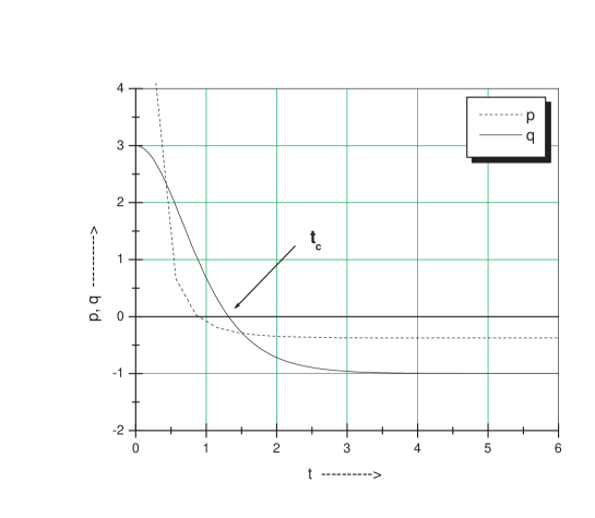
Figure 3: The time evolution of p and q is shown in this figure. When $t>t_{c}$ q becomes negative.

but pressure starts becoming negative earlier at $sinh\omega t>1$. This is not surprising. There is plenty of observational evidence for a decelerating universe in the recent past[26], [27]. But the dominance of negative pressure does not guarantee the present acceleration of the universe. For the universe to accelerate the the negative pressure has to dominate long enough as to overcome the gravitational attraction produced by ordinary matter[28].
Special case ( A= R)
We have mentioned earlier that $A=R$ is a particular solution of the equation (50). Though simple, in what follows, we shall presently see that this choice is rich with various possibilities in interpreting our matter field as also in comparing the evoluon of the universe with a Chaplygin type of fluid.
With $A=R=sinh^{n}\omega t$ we get

$$\rho=6n^{2}\omega^{2}+\frac{6n^{2}\omega^{2}}{sinh^{2}\omega~{}t}=\Lambda+\frac{B}{R^{\frac{2}{n}}}$$ (60)

$$p=-\Lambda-\frac{2n-1}{2n}\frac{B}{R^{\frac{2}{n}}}$$ (61)

where $\Lambda=6n^{2}\omega^{2}$ and $B=\Lambda R_{0}^{\frac{2}{n}}$. One might recall that from equation (4) with $R=A$ and $\gamma=k$ it follows that for, $p=k\rho$ we get

$$\rho=R^{\frac{-1}{4(1+k)}}$$ (62)

such that, $n=\frac{1}{4}$ corresponds to a stiff fluid ( k=1) with $\rho\sim\frac{1}{R^{8}}$ and $n=\frac{2}{5}$ to a radiation dominated phase $(k=\frac{1}{4})$ with $\rho\sim\frac{1}{R^{5}}$ and lastly $n=\frac{1}{2}$ to a matter dominated model(k=0) with $\rho\sim\frac{1}{R^{4}}$. Thus, interesting to point out that the exponent $n$ in equation (64 ) characterises the nature of the fluid we are dealing with. We can make the identification clearer if we write a sort of equation of state using equations (60- 61)as

$$p=\frac{1-2n}{2n}\rho-\frac{\Lambda}{2n}$$ (63)

such that $k=\frac{1-2n}{2n}$. One can now identify the two arbitrary constants in (54) as $\omega=\sqrt{\frac{2\Lambda}{3}}(k+1)$ and $n=\frac{1}{2(k+1)}$ such that we finally get

$$R=R_{0}[\sinh\sqrt{\frac{2\Lambda}{3}}(k+1)t]^{\frac{1}{2(k+1)}}$$ (64)

So we get the following cases of matter field
a. $(n=\frac{1}{4})$ ( stiff fluid)

$$\rho=\Lambda+\frac{B}{R^{8}}~{}~{}and~{}~{}p=-\Lambda+\frac{B}{R^{8}}$$ (65)

b. $(n=\frac{2}{5})$ (radiation)

$$\rho=\Lambda+\frac{B}{R^{5}}~{}~{}and~{}~{}p=-\Lambda+\frac{B}{4~{}R^{5}}$$ (66)

c. $(n=\frac{1}{2})$ ( dust)

$$\rho=\Lambda+\frac{B}{R^{4}}~{}~{}and~{}~{}p=-\Lambda$$ (67)

We see that for small R the equation in case a is approximated by $\rho=\frac{\Lambda}{R^{8}}$, which corresponds to a universe dominated by a stiff fluid in 5D spacetime. Similarly the case b and case c refer to radiation dominated and dust dominated universe respectively. On the other hand for a large value of the cosmological radius we see that the above equations suggest that $\rho=\Lambda~{}~{}and~{}p=-\Lambda$  which, in turn, corresponds to an empty universe with a cosmological constant $\Lambda$ ( i.e., a de Sitter universe)
Thus equations (63-65) describe the mixture of a cosmological constant with a type of fluid obeying some equation of state. The last case known as ’stiff fluid‘ characterised by the equation of state, $p=\rho$ is particularly interesting. Note that a massless scalar field is a particular instance of stiff matter. Therefore, in a generic situation, our cosmology may be looked upon as interpolating between different phases of the universe from a stiff fluid, radiation or dust dominated universe to a de Sitter one passing through an intermediate phase which is a mixture just mentioned above. The interesting point, however, is that such an evolution may be accounted for by using one fluid only as opposed to the earlier works [30],[31] representing simple two fluid model. Correspondence to models driven by a generalised Chaplygin type of fluid [32] described by an equation of state

$$\rho=\left(\Lambda+\frac{B}{R^{3(1+\alpha)}}\right)^{\frac{1}{1+\alpha}}$$ (68)

is only too apparent although here, as mentioned before we do not need to hypothesise the existence of a mysterious type of fluid to explain the observations. Here $\alpha$ is an additional free parameter to play with to fit the observational data. In the light of above discussions the behaviour of the deceleration parameter in our model is as expected (fig.3). Initial dust dominance provides the gravitational pull for the expansion to decelerate but once the cosmological term starts dominating acceleration occurs with, $q=-1$. Although evolution of this kind has been exhaustively discussed in the literature in 4D space time but we are not aware of models of similar kind in higher dimensional spacetime. Moreover we know that for a sheer-free evolution, if the temporal dependence of the scale factor is given, one can construct a potential for a minimally coupled scalar field which would simulate the evolution as with a perfect fluid. Let us illustrate the situation in our model. For the Lagrangian

$$L(\phi)=\frac{1}{2}\dot{\phi^{2}}-V(\phi)$$ (69)

we get the analogous energy density as

$$\rho_{\phi}=\frac{1}{2}\dot{\phi^{2}}+V(\phi)=\Lambda+\frac{B}{R^{\frac{2}{n}}}$$ (70)

and the corresponding ’pressure‘ as

$$p_{\phi}=\frac{1}{2}\dot{\phi^{2}}-V(\phi)=-\Lambda-\frac{B}{R^{\frac{2}{n}}}+\frac{B}{2n~{}R^{\frac{2}{n}}}$$ (71)

such that

$$\dot{\phi^{2}}=\frac{B}{2n~{}R^{\frac{2}{n}}}$$ (72)

which, in turn, gives via equation (5) for flat 4D space

$$\phi^{\prime}=\sqrt{\frac{3B}{n}}\frac{1}{R\sqrt{\Lambda R^{\frac{2}{n}}+B}}$$ (73)

where $\phi^{\prime}$ denotes differentiation w. r. t. the scale factor R. Integrating we get,

$$\phi=\sqrt{\frac{3n}{4}}\ln\frac{\sqrt{B}-\sqrt{\Lambda R^{\frac{2}{n}}+B}}{\sqrt{B}+\sqrt{\Lambda R^{\frac{2}{n}}+B}}$$ (74)

Using equation (54) we finally get

$$\phi=\sqrt{3n}\ln\tanh\frac{\omega t}{2}$$ (75)

On the other hand simple algebra shows that

$$V(\phi)=\Lambda\left(1+\frac{4n-1}{4n}\sinh^{2}\frac{\phi}{\sqrt{3n}}\right)$$ (76)

For the dust case ( $n=\frac{1}{2}$ )

$$V(\phi)=\Lambda\left(1+\frac{1}{2\sinh^{2}\omega t}\right)$$ (77)

while for the analogous stiff fluid case ( $n=\frac{1}{4}$ ) yields a constant potential $V(\phi)=\Lambda=V_{0}$
It may not be out of place to call attention to a quintessential model driven by a tachyonic scalar field [30] with a potential in 4D space time

$$V(T)=\frac{\Lambda}{\sin^{2}\left(\frac{3\sqrt{\Lambda(1+k)}}{2}\right)T}\sqrt{1-(1+k)\cos^{2}\left(\frac{3\sqrt{\Lambda(1+k)}}{2}\right)T}$$ (78)

(T is a tachyonic scalar field) giving the cosmological evolution as

$$R(t)=R_{0}\left(\sinh\frac{3\sqrt{\Lambda}(1+k)t}{2}\right)^{\frac{2}{3(1+k)}}$$ (79)

It behaves like a two fluid model where one of the fluids is a cosmological constant while the other obeys a state equation $p=k\rho$, $(-1<k<1)$. Similarity of this evolution with our model is more than apparent except for some numerical factors coming out because we are here dealing with a higher dimensional spacetime. But the main result may be re-emphasized that we get this evolution without forcing ourselves to invoke any extraneous tachyonic type of scalar field. To end the section a final remark may be in order. From the equation (63) it follows such that the sound speed is given by

$$C_{s}^{2}=\frac{\delta p}{\delta\rho}=\frac{1-2n}{2n}$$ (80)

which implies that to avoid imaginary value of the speed of sound $n<\frac{1}{2}$. Evidently in the dust model $(n=\frac{1}{2})$ $C_{s}$ vanishes as expected. This along with the requirement that $C_{s}$ should never exceed the speed of light further restricts the range of $n$ as $\frac{1}{4}<n<\frac{1}{2}$.

Before concluding the section we call attention to a serious defect of the present analysis. Here we have postulated a 5D matter field. But what is relevant is the effective 4D physical quantities. In line with our discussions in section 4 we can calculate the 4D quantities as $(\rho-\rho_{0})$ and $(p-p_{0})$ in this case also. From equation (5) it follows that with $R=A$ and $d=1$, $\rho_{0}=3\frac{\dot{R^{2}}}{R^{2}}$ such that the expression $(p-p_{0})$ turns out to be qualitatively of the same form as in equation (60). Only the numerical factor differs. So most of our findings remains essentially unaltered, which is hardly surprising because with $R=A$ the radial and the extra fifth coordinate are exactly equivalent. So we are brief on this point.

6. Discussion

In this work we have discussed a 5D homogeneous model with maximally symmetric 3D space. As the field equations are under determined we are forced to assume two equations of state connecting pressure and density. But it should also be emphasised that,for the sake of mathematical simplicity, we have chosen to sacrify some generality and to assume a number of relations in sections 4 and 5 to make the field equations integrable. Nevertheless our solutions are quite general in nature in the sense that many well known results in this field are recovered as special cases. Fixing the magnitude of the arbitrary constants we have ensured the positivity of the matter field, good energy conditions as well as dimensional reduction. We have taken only one extra spatial dimension but we believe most of the findings may be extended if we take a larger number of extra dimensions. The most important finding in this work, in our opinion, may be summarised as : we do not have to hypothesise the existence of an extraneous scalar field with mysterious properties of matter to achieve an accelerating universe. However one should admit that here we have to postulate the existence of an extraneous 5D matter field instead as also some other assumptions to achieve the acceleration. Relevant to point out that in an interesting work Li Quiang etal [10] also recently showed that the Brans Dicke theory generalised to five dimensions is reduced to a 4D theory where the 4-metric is coupled to two scalar fields, which may account naturally for the present accelerated expansion of the universe. The extra matter field in our model is of geometrical origin which is, however, not very uncommon in the literature. Correspondence to curvature quintessence, Wesson’s induced matter theory as also the shadow matter concept of Frolov etal in the context of brane cosmology may be of some relevance here. To end the section we like to point out some serious shortcomings of our model which need considerable refinements in future exercise. In section 5 the model is based on assumption of a specific form of the deceleration parameter, which definitely suffers from the disqualification of a sort of ad-hocism. Moreover the proper interpretation of matter field in higher dimensional models continues to plague the workers in this field. In the cosmological context one starts with a 5D matter field and looks for various types of dynamical compactification of the extra dimensions.It is conjectured that some stabilising mechanism ( quantum gravity may be a potential candidate) should finally halt the continual shrinkage such that it stabilises at a planckian length so as to be unobservable with the low energy physics available today. So with this phase transition the extra metric coefficients lose their dynamical character and the field equations along with the matter field are effectively four dimensional and it enters exactly the 4D FRW phase. So in this scenario there is no effective 4D properties of matter. While some of the solutions in section 3 are amenable to the desirable feature of dimensional reduction in section 5 we have taken the fifth dimension in the same footing with the rest as $R=A$. So dimensional reduction is clearly absent. Apart from this undesirable feature a serious defect of our work is the absence of any stabilising mechanism itself which should finally halt the continual shrinkage of the extra space. In this regard comparison with analogous curvature driven quintessence models are striking where most of the solutions are unstable against perturbations. In that context Guendelman and Kaganovich [33] showed earlier that Wheeler-deWitt equation in ADS space time does provide a quantum repulsive effect to stabilise the extra spatial volume. It is also shown that if one works with more than one extra dimension it may create a repulsive potential to avoid the singularity of zero extra spatial volume [34] ,[35].
To conclude a final remark may be in order. In section 5 the assumtion $R=A$ generates a matter field which may be interpretated as a mixture of perfect fluid obeying an equation of state as well as a cosmological constant with either term dominating at different phases of evolution allowing a smooth transition from a decelerating to an accelerating model. With no dynamical reduction this form of matter field is open to serious criticism as we no longer recover the 4D cosmology nor the effective 4D properties of matter. But both in Wesson’s STM theory or its equivalent brane models [36] it is the effective 4D physics that matters.In fact the acceleration is here made possible because we have introduced a 5D matter at the expense of an extraneous scalar field with peculiar properties. Further when one imposes the cylindricity condition of Kaluza-Klein the induced matter in the STM theory is either radiation-like or empty [37], which certainly can not be the source of acceleration.

As a future exercise one should envisage an additional scenario with other inputs such that the currently observed acceleration is followed by a decelerating phase, which finally hits a big brake singularity.

Acknowledgment : S.C. wishes to thank TWAS, Trieste for travel support and ITP (Beijing) for local hospitality where the work was initiated while DP acknowledges financial support of UGC, New Delhi. We also thank the anonymous referee for comments which led to a significant improvement of the earlier version.

References

- [1] T. Padmanabhan - ‘Understanding our Universe : Current status and open issues’ and references therein, gr- qc / 0503107
- [2] B. M. N. Carter, et al, ‘Type IA supernovae Tests of fractal buble universe with no cosmic acceleration’, astro-ph / 0504192 ;
- [3] Zong-Kuan Guo and Y. Z. Zhang , astro-ph / 0506091
- [4] R. Viswakarma, Mon. Not.R. Astro. Soc. 345, 545 (2003)
- [5] C. Csaba, N. Kaloper, J. Terning, Phys. Rev. Lett. 88, 161302 (2002)
- [6] S. Das, N. Banerjee and N. K. Dadhich, ’Curvature driven acceleration: a utopia or a reality ? ’, astro - ph / 0505096;
- [7] Ujjaini Alam, Varun Sahni and A. A. Starobinsky, J. Cosm. and Astr. Part. Phy. 0406, 008 (2004)
- [8] S. Chatterjee, A. Banerjee and Y. Z. Zhang, gr-qc 0509112 Int. J. Mod. Phy. A21,4035 (2006);
- [9] B. Cuadros- Melgar and E. Papantonopoulos, Brazilian J. Phys.35, 1117 ( 2005);
- [10] Li Qiang, Yongge Ma, Moxin Han and Dan Yu, Phys. Rev.D71, 061501 (R), 2005.
- [11] Wesson P. S. Space-Time-Matter, World Scientific, Singapore(1999);
- [12] S. Chatterjee, B. Bhui, Mon. Not.R. Astro. Soc. 247, 577 (1990)
- [13] A. Einstein, The Meaning of Relativity ( Princeton Univ. Press, Princeton, 1956 ); J. A. Wheeler, ‘Einstein’s Vision’, Springer, Berlin (1968)
- [14] K.A. Milton,‘Dark energy as Evidence for extra dimensions’ OK - HEP - 02-08.
- [15] N. Mohammedi, Phys. Rev. D65, 104018, (2002)
- [16] S. Randjber-Daemi, Salam A. and J. Strathdee, Phys. Lett. 135B, 388 (1984)
- [17] A. Chodos and S. Detweiler, Phy. Rev. D21, 2167 (1980)
- [18] O. Grøn, Astronomy Ashtrophysics 193, 1 (1988)
- [19] A. Banerjee, D. Panigrahi and S. Chatterjee, Class. Quant. Grav. 11, 1405 (1994)
- [20] H. Ishihara, Prog. Theor. Phys. 72, 376 (1984);
- [21] Alvarez E and Gavela M, Phys. Rev. Lett. 51, 931 (1983)
- [22] A. G. Riess,‘The case for an accelerating universe from supernovae’, astro-ph / 0005229.
- [23] C. Csaki, hep- ph/ 0404096.
- [24] J. Hewlett and M. Spiropulu, Ann. Rev. Nucl part. Sci.52, 397 92002).
- [25] P. Frolov, M. Snajdr, D. Stojkovic, Phy. Rev. D68, 044002 (2003)
- [26] A. G. Riess et al , Astro. Phys. Journal 560, 49 (2001);
- [27] M. S. Turner, A Riess, Astro. Phys. Journal 569, 18 (2002)
- [28] J. Ponce de Leon, Gen. Rel. Grav.38, 61 (2006)
- [29] Sanjeev S. Seahra and P. S. Wesson, Class. Quantum Grav.20, 1321 (2003)
- [30] V. Gorini, A. Kamenshchik, U. Moschella and V. Pasquier, ‘Tachyons, scalar fields and cosmology’, hep-th / 0311111;
- [31] J. D. Barrow, Phys. Lett.B235, 40 (1990)
- [32] M. C. Bento, O. Bertolami and A. A. Sen, Phy. Rev.D66, 043507 (2002).
- [33] E. I. Guendelman and A. B. Kaganovich , Phys. Rev. D2, 221 (1993)
- [34] U Gunther and A. Zhuk , Phys. Rev. D61, 124001 (2000);
- [35] U Gunther and A. Zhuk ,Proc. 10th Marcel Grossmann Meet ( Rio ), Pt B, p 877 (World Sceintific 2005)
- [36] J. Ponce de Leon, Mod.Phys.Lett.A16, 2291 (2001)
- [37] P. S. Wesson & J. Ponce de Leon, J.Math. Phys.33, 3883 (1992)