On-ground tests of LISA PathFinder thermal diagnostics system

Abstract

Thermal conditions in the LTP, the LISA Technology Package, are required to be very stable, and in such environment precision temperature measurements are also required for various diagnostics objectives. A sensitive temperature gauging system for the LTP is being developed at IEEC, which includes a set of thermistors and associated electronics. In this paper we discuss the derived requirements applying to the temperature sensing system, and address the problem of how to create in the laboratory a thermally quiet environment, suitable to perform meaningful on-ground tests of the system. The concept is a two layer spherical body, with a central aluminium core for sensor implantation surrounded by a layer of polyurethane. We construct the insulator transfer function, which relates the temperature at the core with the laboratory ambient temperature, and evaluate the losses caused by heat leakage through connecting wires. The results of the analysis indicate that, in spite of the very demanding stability conditions, a sphere of outer diameter of the order one metre is sufficient. We provide experimental evidence confirming the model predictions.

1 Introduction

LISA Pathfinder (LPF) is an ESA mission, with NASA contributions, whose main objective is to put to test critical parts of LISA (Laser Interferometer Space Antenna), the first space borne gravitational wave (GW) observatory [1]. The science module on board LPF is the LISA Technology Package (LTP) [2], which basically consists in two test masses in nominally perfect geodesic motion (free fall), and a laser metrology system; this one detects residual deviations of the test masses’ actual motion from the ideal free fall, to a given level of accuracy [3].

In order to ensure that the test masses are not deviated from their geodesic trajectories by external (non-gravitational) agents, a so called Gravitational Reference System (GRS) is used [4]. This consists in position sensors for the masses which send signals to a set of micro-thrusters; the latter take care of correcting as necessary the spacecraft trajectory, so that at least one of the test masses remains centred relative to the spacecraft at all times. The combination of the GRS plus the actuators is known as drag-free subsystem.

The drag-free is of course a central component of LISA, and needs to be operated at extremely demanding levels of accuracy. The laser metrology system should then be sufficiently precise to measure relative test mass deviations. The overall level of noise acceptable for LISA is defined in terms of rms acceleration spectral density, and has been set to [1]

$$S_{a,{\rm LISA}}^{1/2}(\omega)\leq 3\!\times\!10^{-15}\,\left[1+\left(\frac{\omega/2\pi}{3\ {\rm mHz}}\right)^{\!\!2}\right]\,{\rm m}\,{\rm s}^{-2}/\sqrt{\rm Hz}$$ (1)

in the frequency range $0.1\,{\rm mHz}\leq\omega/2\pi\leq 100\,{\rm mHz}$. This is equivalent to $S_{h}^{1/2}$ $\sim$ $4\times 10^{-21}$ Hz^-1/2, with the same frequency dependence.

LPF is conceived, as mentioned above, as an in-flight test of key technologies for LISA. Top level performance requirements for LPF have however been relaxed by an order of magnitude relative to LISA, both in noise amplitude and in frequency band, to still challenging goals [5]:

$$S_{a,{\rm LPF}}^{1/2}(\omega)\leq 3\!\times\!10^{-14}\,\left[1+\left(\frac{\omega/2\pi}{3\ {\rm mHz}}\right)^{\!\!2}\right]\,{\rm m}\,{\rm s}^{-2}/\sqrt{\rm Hz}$$ (2)

in the frequency range $1\,{\rm mHz}\leq\omega/2\pi\leq 30\,{\rm mHz}$. We shall be referring to this frequency band as the LTP Measuring Bandwidth (MBW) in the sequel.

Equation (2) gives the global noise budget. This is made up of contributions from various perturbative agents, both of instrumental and environmental origin. One of these is temperature fluctuations, for which a stability requirement has been set to

$$S_{T}^{1/2}(\omega)\leq 10^{-4}\,{\rm K}/\sqrt{\rm Hz}\ ,\quad 1\,{\rm mHz}\leq\omega/2\pi\leq 30\,{\rm mHz}$$ (3)

in order to comply with (2) under suitable noise apportioning criteria —see section 2.

Because temperature stability is important, a decision has been taken to place high precision thermometers in several strategic spots across the LTP—as part of what is called Diagnostics Subsystem [6] . Such high precision temperature measurements will be useful to identify the fraction of the total system noise which is due to thermal fluctuations only, and this will in turn provide important debugging information to assess the performance of the LTP [7].

The best temperature sensors for our purposes are electric devices whose ohmic resistance varies with temperature. We have chosen to use thermistors, which are semiconductor resistors whose resistance decreases as their temperature increases [8], because they have a rather steep sensitivity curve, and this suits our needs. Such sensors need additional electronic circuitry to bias them and acquire data. The entire chain of sensors plus electronics must of course be tested in ground before boarding, and this requires suitably stable environmental conditions in the first place.

This paper addresses the problem of which are these conditions, and how to implement them for a reliable laboratory test of the LTP temperature sensors and electronics. It is organised as follows: in section 2 we review and quantify the identified sources of thermal noise which result in the budget given in equation (3). In section 3 we discuss how the stability requirement results in a requirement on the temperature system performance, and extend the argument to make precise the environmental conditions which must be met in the laboratory test. In section 4 we present the physical hypotheses, lay down the mathematical model of the proposed insulation scheme, and find an analytic solution to the equations. We then address in section 5 the numerical implications of the above for realistic situations, including a discussion of heat leakage through connecting wires. Section 6 deals with the experimental verification of the model predictions, and section 7 summarises our conclusions and future prospects. Some supplementary mathematical detail is provided in an appendix.

2 Thermal disturbances in the LTP

Temperature fluctuations inside the LTP result in noisy readout at the interferometer output port —the phasemeter. The reason for this is that there are components in the LTP whose behaviour is sensitive to temperature changes, as we shall describe in this section.

As a rule of thumb, the total contribution of thermal noise to the total acceleration noise, equation (2), should not exceed 10 %. We thus require that

$$S_{a,{\rm thermal}}^{1/2}(\omega)\leq 3\!\times\!10^{-15}\,\left[1+\left(\frac{\omega/2\pi}{3\ {\rm mHz}}\right)^{\!\!2}\right]\,{\rm m}\,{\rm s}^{-2}/\sqrt{\rm Hz}$$ (4)

for frequencies within the LTP MBW. This assumption is in fact somewhat conservative, as the Project Engineers have estimated that more than twice this value is actually compliant with the overall LTP noise budget [9]. We shall however adopt equation (4) as reference to ensure we are playing on the safe side.

For the sake of clarity, we consider separately the influence of temperature on the GRS and on the Optical Metrology System (OMS).

2.1 Noise effects inside the GRS

Temperature differences between the walls of the electrode housing cause differential pressures on opposite faces of the test masses, which in turn result in net forces on them, hence in noise at the phasemeter.

Three different mechanisms have been identified whereby temperature fluctuations distort the LTP readout: radiation pressure, radiometer effect and outgassing. Let us briefly describe each of them, and quantitatively estimate their respective contributions to thermal noise.

2.1.1 Radiation pressure

A body at any (absolute) temperature $T\/$ emits thermal radiation. This exerts pressure on any surfaces the radiation hits. According to standard electromagnetic theory, such pressure is given by

$$p_{\rm e.m.}=\frac{4}{3}\,\frac{\sigma}{c}\,T^{4}$$ (5)

where $\sigma$ = 5.67$\times$10^-8 Wm^-2K^-4 is the Stefan-Boltzmann constant, and $c\/$ is the speed of light. Thus, if there are temperature fluctuations around the test mass, a noisy net force will appear on it —see Figure 1 for a graphical display. The effect can be easily quantified making use of equation (5):

$$\Delta p_{\rm e.m.}=\frac{16\,\sigma}{3\,c}\,T^{3}\Delta T$$ (6)

where $\Delta p\/$ and $\Delta T\/$ make reference to differences of pressure and temperature between the sides of the test mass. Associated acceleration noise is hence obtained multiplying the above by the test mass surface area, $\ell_{\rm TM}^{2}$ and dividing by its mass $m_{\rm TM}$:

$$\Delta a_{\rm e.m.}=\frac{16\,\ell_{\rm TM}^{2}\sigma}{3\,m_{\rm TM}c}\,T^{3}\Delta T$$ (7)

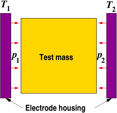
Figure 1: Schematics of the effect of different pressures on opoosite faces of a test mass. The physical origin of pressure differences is explained in the text.

2.1.2 Radiometer effect

This is an effect which happens in rarefied gas atmospheres, its name historically coming from its association with the theory of Crookes’s lightmill radiometer. In low pressure atmospheres, where the gas particles have a mean free path well in excess of the dimensions of the containing vessel, equilibrium conditions do not happen when pressure is uniform, but rather when the ratios of pressure to square root of temperature equal one another. Or [10],

$$\frac{p_{1}}{\sqrt{T_{1}}}=\frac{p_{2}}{\sqrt{T_{2}}}$$ (8)

The pressure gradient is readily obtained from this expression, and thence the associated test mass acceleration:

$$\Delta a_{\rm radiometer}=\frac{1}{2}\,\frac{p\,\ell_{\rm TM}^{2}}{m_{\rm TM}}\,\frac{\Delta T}{T}$$ (9)

2.1.3 Outgassing

Outgassing is one of the causes of the presence of gas within the walls of the GRS. In the present contetx, outgassing problems actually derive from temporal fluctuations in its rate, which once more result in pressure fluctuations, thence in noise. Outgassing rates are very strongly dependent on materials and geometry, and the theoretical analysis of the problem is by no means a simple one. The issue has also attracted attention of people from other space missions [11], and further experimental work appears to be necessary to reliably assess the impact of this phenomenon. Partial evidence has however been gathered that outgassing might be in practice a small effect in the LTP [12]. We shall therefore omit any further consideration of this phenomenon here.

2.1.4 Total thermal noise in the GRS

If we make the assumption that radiometer and radiation pressure fluctuations are uncorrelated, and neglect outgassing, then equations (7) and (9) are added quadratically, and hence the spectral densities of acceleration and temperature in the GRS are related by

$$S_{a,{\rm thermal\ GRS}}^{1/2}(\omega)=\sqrt{\left(\frac{16\,\ell_{\rm TM}^{2}\sigma}{3\,m_{\rm TM}c}\,T^{3}\right)^{\!\!2}+\left(\frac{p\,\ell_{\rm TM}^{2}}{2m_{\rm TM}}\,T^{-1}\right)^{\!\!2}}\;S_{T,\ GRS}^{1/2}(\omega)$$ (10)

Nominal conditions in the LTP are the following:

$\ell_{\rm TM}=4.6\times 10^{-2}$ m

${m_{\rm TM}}=1.96$ kg

$T=293$ K

$p=10^{-5}$ Pa

which give

$$S_{T,\ GRS}^{1/2}(\omega)=3.3\times 10^{10}\;S_{a,{\rm thermal\ GRS}}^{1/2}(\omega)\ {\rm K\,Hz}^{-1/2}$$ (11)

This expression gives 0.9 $\times$ 10^-4 K/$\sqrt{\rm Hz}$ in the worst case that all the thermal acceleration budget, equation (4), is allocated to thermal fluctuations in the GRS.

2.2 Noise effects inside the OMS

The Optical Metrology System of the LTP is based on a non-polarising, heterodyne Mach-Zender interferometer [13]. The light source is an infrared Nd:YAG laser of 1.064 $\mu\/$m wavelength and approximately 0.25 W of power. Optical components are mounted on an optical bench of highly stable optical properties. Temperature fluctuations basically affect the optical system through two distinct effects [14]:

• The index of refraction of optical components depends on temperature.

• Temperature changes cause dilatations (and contractions) of optical elements, which in turn cause light’s optical path to change accordingly.

While it is not difficult to characterise how individual components are influenced by the above effects, to assess the behaviour of the fully integrated optical metrology is a more complicated task. Significant progress has been made since the early design proposals —see reference [2] and following articles in that issue of CQG—, and improved materials and designs are now available. Altogether, it appears that

$$S_{T,\ {\rm OMS}}^{1/2}\simeq 10^{-4}\,{\rm K}/\sqrt{\rm Hz}$$ (12)

is a sensible requirement which should comfortably guarantee the performance of the optical bench against temperature fluctuations in flight —see [14], chapter 12, and [15]. Like before, the noise level (12) is estimated to account for about 10 % of the total LTP acceleration noise, equation (4).

2.3 Total thermal noise budget for the LTP

If we make the hypothesis that noise in the OMS is uncorrelated with noise in the GRS then the respective spectral densities add up, i.e.,

$$S_{T}(\omega)=S_{T,\ GRS}(\omega)+S_{T,\ OMS}(\omega)$$ (13)

Inserting here equations (11) and (12), we find that the LTP thermal stability must be

$$S_{T}^{1/2}(\omega)\simeq 1.3\times 10^{-4}\,{\rm K}/\sqrt{\rm Hz}$$ (14)

where the usual frequency dependence of equation (2) has been dropped, as it is in practice the case that temperature fluctuations actually drop towards higher frequencies —due to efficient thermal insulation of the LTP.

The number just obtained is very close to that of equation (3), and derived under worst hypotheses in each case. We are thus reassured that equation (3) is a sensible requirement for the temperature fluctuations which can be tolerated in the LTP. Let us however stress that we still can count with some margin, as acceleration thermal noise allocation has been taken as a conservative 10 % of the total acceleration noise —see paragraph following equation (4).

3 Temperature measurement and on-ground test requirements

Temperature stability requirements for the LTP are now established. We rewrite them again:

$$S_{T}^{1/2}(\omega)\leq 10^{-4}\,{\rm K}/\sqrt{\rm Hz}\ ,\quad 1\,{\rm mHz}\leq\omega/2\pi\leq 30\,{\rm mHz}$$ (15)

Because this is a requirement, satellite and payload will be built such that thermal conditions in the LTP meet (15). Even so, to monitor the magnitude of anyway compliant temperature fluctuations is a powerful diagnostic tool, yielding valuable information on the system thermal behaviour, which will be useful for LISA. In addition, we wish to be able to diagnose whether the conditions (15) actually prevail at any given time during the mission. For both objectives, temperature gauges are obviously needed.

We now pose the question: which is the level of noise we can accept in the temperature measurement system —which includes sensors, wires and electronics— if we are to diagnose temperature variations below the level (15)? Clearly, the answer to that question depends on how accurately those fluctuations are to be measured. The stability requirement equation (15) is already rather demanding of itself, so we do not expect thermal fluctuations to be much smaller. With this in mind, to request the measuring system to be about one order of magnitude less noisy than the maximum noise level to measure seems a sensible option:

$$S_{T,\ {\rm measurement}}^{1/2}(\omega)\leq 10^{-5}\,{\rm K}/\sqrt{\rm Hz}\ ,\quad 1\,{\rm mHz}\leq\omega/2\pi\leq 30\,{\rm mHz}$$ (16)

This has in fact become a mission top level requirement —see [5], section 6.2. There are two groups of reasons which support it:

1. Equation (15) defines the maximum acceptable level of temperature noise in the LTP. If this is satisfied, which of course must, then actual fluctuations will be less than that. Requirement (16) then sets a 10 % minimum discrimination capability for the measuring device, a standard approach which is certainly compatible with better performance.

2. LISA is more demanding than LPF as regards thermal stability. Actually, LISA requires an order of magnitude less thermal noise than LTP [14]. If we require (16) for LTP then we are in a position where analysis of thermal sources of noise of relevance for LISA can be identified and tagged for improvement, at least in the overlapping frequency band of both missions. This prospect is in line with the very concept of LPF as a precursor mission.

3.1 Absolute versus differential temperature measurements in flight

The above arguments, and specially the first, can perhaps be critisised in terms of: why not perform differential measurements? This might relax the very demanding requirement in equation (16), in the sense that it would only apply to differential rather than absolute temperature measurements in flight.

While it is true that certain thermal disturbances depend on temperature gradients across the test masses —like the radiometer effect and radiation pressure gradients— there are others which do not —mostly those related to the optics. One could accordingly split up the temperature gauges into two classes, but this does not seem a particularly sensible choice, since the best device would obviously be the one to use in all cases, anyway.

A space mission like LPF does not generally allow to fix hardware design inefficiencies once it has been launched. The choice of making applicable the requirement stated in equation (16) to all temperature measurements, whether differential or absolute, seems thus not advisable to relax: some margin is necessary to cope with unforseen sources of error.

3.2 Environmental conditions for on-ground tests

Before launch, the temperature diagnostics hardware must be tested in ground. In order to do a meaningful test, a sufficiently stable thermal environment must be granted for the sensors in the first place. Here, sufficiently stable means that any observed fluctuations in the readout data should be attributable solely to sensor and/or electronics noise, rather than to a combination of the latter with ambient temperature fluctuations. This means ambient temperature fluctuations in the thermometers should be distinctly smaller than the limit set by the the requirement, equation (16). Again, one order of magnitude below that target sensitivity seems a good prescription. So we require

$$S_{T,\ {\rm testbed}}^{1/2}(\omega)\leq 10^{-6}\,{\rm K}/\sqrt{\rm Hz}\ ,\quad 1\,{\rm mHz}\leq\omega/2\pi\leq 30\,{\rm mHz}$$ (17)

It turns out that 10${}^{-6}\,{\rm K}/\sqrt{\rm Hz}$ is a very demanding temperature stability, orders of magnitude beyond the capabilities of thermally regulated rooms. Once more, this figure could be widely relaxed if tests were done differentially, i.e., between pairs of sensors close enough to one another. While such differential measurements are indeed envisaged, we also want to make sure that the sensing system is sensitive enough that absolute temperature measurements are compliant with the most exigent requirements. We thus adopt equation (17) as the design goal baseline.

The concept idea of the insulator is displayed in figure 2: an interior metal core of good thermal conductivity is surrounded by a thick layer of a poorly conductive material. The inner block ensures thermal stability of the sensors attached to it, while the surrounding substrate efficiently shields them from external temperature fluctuations in the laboratory ambient. We propose a spherical shape for the sake of simplicity of the mathematical analysis, even though this will be eventually changed to cubic in the actual experimental device for practical reasons.

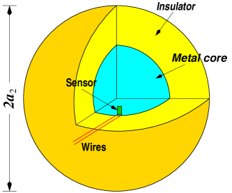
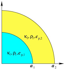
Figure 2: Thermal insulator design concept. Left: 3D diagramme, including sensor placement principle. Right: cut view, with notation convention dictionary.

4 Mathematical model of the insulator

The basic assumption of the mathematical analysis we shall present is that heat flows from the interior of the insulator to the air outside, and from the latter to the interior of the insulator, only by thermal conduction. This is a very realistic hypothesis in the context of the experiment, as radiation mechanisms are certainly negligible and convection should not play any significant role, either, since the entire body is solid, and temperature fluctuations will be small anyway.

Let then $T({\bf x},t)$ be the temperature at time $t\/$ of a point positioned at vector x relative to the centre of the sphere. Under the conduction-only hypothesis, $T({\bf x},t)$ satisfies Fourier’s partial differential equation [16]

$$\rho c_{\rm p}\,\frac{\partial}{\partial t}T({\bf x},t)=\nabla\cdot\left[\kappa\nabla T({\bf x},t)\right]$$ (18)

where $\rho$, $c_{\rm p}$ and $\kappa$ are the density, specific heat and thermal conductivity, respectively, of the substrate. We shall assume these are uniform values within each of the two materials making up the insulating body, with abrupt changes in the interface. We can thus represent them as discontinuous functions of the radial coordinate, as follows:

$$\rho,c_{\rm p},\kappa({\bf x})=\left\{\begin{array}[]{ll}\rho_{1},c_{{\rm p}1},\kappa_{1}&{\rm if}\ \ 0\leq r<a_{1}\\ \rho_{2},c_{{\rm p}2},\kappa_{2}&{\rm if}\ \ a_{1}\leq r<a_{2}\end{array}\right.$$ (19)

with $r\/$ $\equiv$ $|{\bf x}|$. Initial and boundary conditions are the following:

$$T({\bf x},t=0)=0\ ,\quad T(r=a_{2},t)=T_{0}(\theta,\varphi;t)$$ (20)

where $\theta\/$ and $\varphi\/$ are spherical angles which define positions on the sphere’s surface. The boundary temperature can be expediently expressed as a multipole expansion:

$$T_{0}(\theta,\varphi;t)=\sum_{lm}\,b_{lm}(t)\,Y_{lm}(\theta,\varphi)$$ (21)

where $Y_{lm}(\theta,\varphi)$ are spherical harmonics, and $b_{lm}(t)$ are boundary multipole temperature components.

In practice, the boundary temperature will be randomly fluctuating, therefore $b_{lm}(t)$ will be considered stochastic functions of time. We shall also reasonably assume them to be stationary Gaussian noise processes with known spectral densities, $S_{lm}(\omega)$.

As shown in the appendix, the frequency analysis of this problem leads to a transfer function expression of the temperature inside the body:

$$\tilde{T}({\bf x},\omega)=\sum_{lm}\,H_{lm}({\bf x},\omega)\,\tilde{b}_{lm}(\omega)$$ (22)

where tildes ( $\tilde{}$ ) stand for Fourier transforms, e.g.,

$$\tilde{T}({\bf x},\omega)\equiv\int_{-\infty}^{\infty}\,T({\bf x},t)\,e^{-i\omega t}\,dt$$ (23)

etc. If we make the further assumption that different multipole temperature fluctuations at the boundary are uncorrelated, i.e.,

$$\langle\tilde{b}^{*}_{l^{\prime}m^{\prime}}(\omega)\,\tilde{b}_{lm}(\omega)\rangle=S_{lm}(\omega)\,\delta_{l^{\prime}l}\,\delta_{m^{\prime}m}$$ (24)

then the spectral density of fluctuations at any given point inside the insulating body is given by

$$S_{T}({\bf x},\omega)=\sum_{lm}\,\left|H_{lm}({\bf x},\omega)\right|^{2}\,S_{lm}(\omega)$$ (25)

It is ultimately the spectral density $S_{T}({\bf x},\omega)$, for $|{\bf x}|$ $\leq$ $a_{1}$, which has to comply with the requirement expressed by equation (17). Based on knowledge (by direct measurement) of ambient laboratory temperature fluctuations, equation (25) will provide the guidelines, as regards materials and dimensions, for the actual design of a suitable insulator jig.

4.1 Isotropic boundary conditions

Thermal conditions in the laboratory are rather homogeneous. This means that the boundary temperature fluctuations will be in practice essentially independent of the angles $\theta\/$ and $\varphi$, i.e.,

$$T_{0}(\theta,\varphi;t)=B(t)$$ (26)

and consequently the generic expansion equation (21) includes only the monopole term. Hence

$$b_{00}(t)=\sqrt{4\pi}\,B(t)$$ (27)

The temperature $T({\bf x},\omega)$ in this case will only depend on radial depth, $r$, and therefore

$$\tilde{T}(r,\omega)=H(r,\omega)\,\tilde{B}(\omega)$$ (28)

with $H(r,\omega)$ $\equiv$ $\sqrt{4\pi}\,H_{00}({\bf x},\omega)$. According to equation (59) of the Appendix, this is

$$H(r,\omega)=\left\{\begin{array}[]{ll}\xi_{0}(\omega)\,j_{0}(\gamma_{1}r)\ ,&0\leq r\leq a_{1}\\[5.16663pt] \eta_{0}(\omega)\,j_{0}(\gamma_{2}r)+\zeta_{0}(\omega)\,y_{0}(\gamma_{2}r)\ ,&a_{1}\leq r\leq a_{2}\end{array}\right.$$ (29)

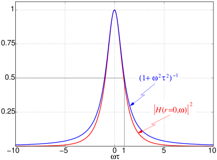
Figure 3: Frequency response at the centre ($r\/$ = 0) of a spherical thermal insulator —as given in equation (29)—, along with the frequency response of a low-pass filter of order one and same frequency cut-off, $\omega_{\rm cut-off}$ = $1/\tau$.

This is a low-pass filter transfer function —even though the cumbersome frequency dependencies involved in the expressions above do not make it immediately obvious. The 3 dB cut-off angular frequency for this filter defines a time constant $\tau$ by $1/\tau$ $\equiv$ $\omega_{\rm cut-off}$, which correspondingly is a complicated function of the insulator’s physical and geometrical properties. Figure 3 shows graphically the situation: the red curve plots the square modulus of $H(r=0,\omega)$, where the cut-off $1/\tau$ is shown as the 3 dB abscissa. For comparison, the figure also shows (blue curve) a low-pass filter of the first order with the same frequency cut-off, i.e., $|H_{\rm 1st\ order}(\omega)|^{2}$ = $(1+\omega^{2}\tau^{2})^{-1}$.

The high frequency roll-off of the real filter (in red) is seen to drop below the first order counterpart (in blue): the latter clearly has a slow slope at high frequencies, $|H_{\rm 1st\ order}(\omega)|$ $\sim$ $(\omega\tau)^{-1}$, while the former can be shown to follow a much steeper, exponential curve:

$$|H(0,\omega)|\sim\omega\tau\,e^{-\sqrt{\omega\tau}}\quad{\rm when}\ \ \omega\tau\gg 1$$ (30)

As already mentioned in section 1, to test the temperature sensors and electronics we need a very strong noise suppression factor in the LTP frequency band. Inspection of figure 3 and equation (30) readily shows that high damping factors require such frequency band to lie in the filter’s tails. The thermal insulator should therefore be designed in such a way that its time constant $\tau\/$ be sufficiently large to ensure that the LTP MBW frequencies are high enough compared to $(2\pi\tau)^{-1}$. The exponential roll-off in the transfer function shown by (30) makes the filter actually feasible with moderate dimensions.

5 Numerical analysis

In this section we consider the application of the above formalism to obtain useful numbers for the implementation of a real insulator device which complies with the needs of the experiment.

First of all, a selection of an aluminium core surrounded by a layer of polyurethane was made. Aluminium is a good heat conductor and is easy to work with in the laboratory; polyurethane is a good insulator and is also convenient to handle, as it can be foamed to any desired shape from canned liquid. Other alternatives are certainly possible, but this appears sufficiently good and we shall therefore stick to this specific choice. The relevant physical properties of aluminium and polyurethane are as follows:

	Density	Specific heat	Thermal conductivity
	$\rho$ (kg m-3)	$c_{\rm p}$ (J kg-1 K-1)	$\kappa$ (W m-1 K-1)
Aluminium	2700	900	250
Polyurethane	35	1000	0.04

Figure 4 plots the amplitude damping coefficient of the insulator block, $|H(r,\omega)|$, at the lower end of the LTP frequency band (i.e., 1 mHz) at the interface position, $r\/$ = $a_{1}$. Each of the curves corresponds to a fixed value of the latter, and is represented as a function of the outer radius of the insulator. This choice is useful because the sensors are implanted for test on the surface of the aluminium core, and also because at higher frequencies thermal damping is stronger. The plot clearly shows that the assymptotic regime of equation (30) is quite early established.

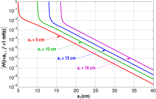
Figure 4: Amplitude damping factor on the interface between aluminium and polyurethane at 1 mHz, for various sizes of the insulating device.

The choice of dimensions for the insulating body must of course ensure that the minimum requirement, equation (17) is met. For this, a primary consideration is the size of the ambient temperature fluctuations in the site where the experiment is made. Dedicated measurements in our laboratory showed that

$$S_{T,\ {\rm room}}^{1/2}(\omega)\simeq 10^{-1}\,{\rm K}/\sqrt{\rm Hz}\ ,\quad 1\,{\rm mHz}\leq\omega/2\pi\leq 30\,{\rm mHz}$$ (31)

We therefore need to implement a device such that $|H(a_{1},\omega)|$ $\leq$ 10^-5 throughout the MBW. Suitable dimensions can then be readily read off figure 4, and various alternatives are possible, as seen. Before making a decission, however, we need to make an additional estimate of the heat leakage down the electric wires which connect the temperature sensors with the electronics, which lies of course outside the insulator. We come to this next.

5.1 Heat leakage through connecting wires

We use a simple model, consisting in assuming the connecting wires behave as straight thin rods which connect the central aluminium core with the electronics, placed in the external laboratory ambient. Because the polyurethane provides a very stable insulation, we can neglect the lateral flux, hence only a unidimensional heat flow needs to be considered. For this, the following equation relates the heat flux to the temperature difference between the two wires’ edges:

$$\dot{Q}(t)=\kappa_{\rm wire}\,\frac{\pi R_{\rm wire}^{2}}{\ell_{\rm wire}}\;[T(a_{2},t)-T(a_{1},t)]$$ (32)

where $\kappa_{\rm wire}$ is the thermal conductivity of the wire, $R_{\rm wire}$ its transverse radius, and $\ell_{\rm wire}$ its length inside the polyurethane layer.

On the other hand, the heat flux results in temperature variations in the metal core, given by

$$\dot{Q}(t)=\rho_{1}c_{{\rm p}1}V_{1}\,\frac{\partial T}{\partial t}(a_{1},t)$$ (33)

where $V_{1}$ = $4\pi a_{1}^{3}/3$ is the volume of the metal core. Equating the above expressions we find

$$\kappa_{\rm wire}\,\frac{\pi R_{\rm wire}^{2}}{\ell_{\rm wire}}\;[T(a_{2},t)-T(a_{1},t)]=\rho_{1}c_{{\rm p}1}V_{1}\,\frac{\partial T}{\partial t}(a_{1},t)$$ (34)

For fluctuating temperatures, we can now obtain the relationship between the spectral density at the aluminium core and the ambient, caused by heat conduction along the wire:

$$S_{T,\ {\rm wire}}^{1/2}(a_{1},\omega)=|H_{\rm wire}(\omega)|\,S_{T,\ {\rm ambient}}^{1/2}(\omega)$$ (35)

where

$$|H_{\rm wire}(\omega)|\simeq\frac{\pi}{\omega}\,\frac{\kappa_{\rm wire}\,R_{\rm wire}^{2}}{\rho_{1}c_{{\rm p}1}V_{1}\,\ell_{\rm wire}}$$ (36)

and where the approximation has been made that the temperature fluctuations at the inner end of the wire are much smaller than those at the outer end, due to the presence of the polyurethane layer.

In practice, there will be several sensors for test inside the insulator. Under the hypothesis made that no lateral heat flux is relevant, the transfer function for a bundle of $N\/$ of wires is, at most, $N\/$ times that of a single wire. Thus,

$$|H_{N{\rm wires}}(\omega)|=\frac{3N}{\omega/2\pi}\,\frac{\kappa_{\rm wire}\,R_{\rm wire}^{2}}{8\pi\rho_{1}c_{{\rm p}1}a_{1}^{3}\,\ell_{\rm wire}}$$ (37)

Let us consider numerical values in this expression. We use thin copper wires ($\kappa_{\rm Cu}$ = 401 Wm^-1K^-1) of radius $R_{\rm wire}$ = 0.1 mm, and assume some fiducial parameters for the size of the aluminium core, $a_{1}$, the wire length, $\ell_{\rm wire}$, the number of connecting wires, $N$, and the frequency, $\omega/2\pi$. The following obtains:

$$|H_{N{\rm wires}}(\omega)|=1.1\times 10^{-5}\,\left(\frac{N}{30}\right)\!\left(\frac{a_{1}}{13\ {\rm cm}}\right)^{\!-3}\!\left(\frac{\ell_{\rm wire}}{25\ {\rm cm}}\right)^{\!-1}\!\left(\frac{\omega/2\pi}{1\ {\rm mHz}}\right)^{\!-1}$$ (38)

This result indicates that, for laboratory fluctuations in the level of equation (31), leakage through wiring causes fluctuations in the temperature sensors of about 10^-6 K/$\sqrt{\rm Hz}$, equation (35), which is compliant with the requirement of stability, equation (17). The most sensitive parameter in the above expression is the size of the metal core, and this determines the need to make it somewhat large. The length of the wires has been taken to be 25 cm, but this does not necessarily mean we need $a_{2}$ = 38 cm (assuming the radius of the aluminium core is $a_{1}$ = 13 cm), because the wires can be partly wound inside the polyurethane layer to further protect the system against leakage. In fact, wire lengthening is an easy way to improve attenuation.

As regards frequency dependence, compliance is guaranteed in the entire MBW if it is at its lower end: indeed, not only $|H_{\rm wire}(\omega)|$ decreases as $\omega^{-1}$ —see equation (38)—, also ambient noise fluctuations happen to drop below 10^-1 K/$\sqrt{\rm Hz}$ at higher frequencies.

6 Experimental verification

Direct experimental verification of the predicted performance of the insulator would require the sensing system, i.e., sensors plus electronics, to have a level of noise below 10^-6 K/$\sqrt{\rm Hz}$ in the MBW. The requirement on the latter is however 10^-5 K/$\sqrt{\rm Hz}$, and this is itself to be put to test.

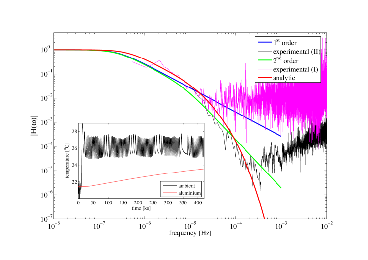
Figure 5: Two insulator transfer functions estimated (noisy curves) and fits to them in the lower frequencies (thicker lines). The inset contains data for the black curve —see text for details.

We shall nevertheless argue that the thermal environment of the sensors produced by the insulator is in fact better than required. Evidence of this comes from rounds of measurements made over periods of several days to weeks, as we now describe.

Already processed data are displayed in figure 5. The noisy curves are estimates of the insulator transfer function as derived from two different experimental runs: the magenta curve corresponds to a data stream about a month long and in largely varying thermal conditions outside the insulator; the black curve corresponds to a shorter time series (five days) which began with an abrupt temperature transient, followed by a periodic signal of a few fractions of a milli-Hertz, —see figure inset. These curves are relatively clean below 10^-4 Hz but they (noisily) tend to approach unity at higher frequencies, which is an indication that electronic noise is dominant in that band: indeed, system readouts inside and outside the insulator tend to equal each other (transfer function nearing unity), while real temperature fluctuations obviously do not.

The thicker lines are fits to the data in the lower frequency band: the red is the exact prediction of the model, while the blue is a first order filter fit, and the green is a second order filter fit. The last two are provided as examples that the data can also be adjusted by simpler models in restricted data regions yet indicating that the actual behaviour of the insulator follows a trend with a steeper slope towards higher frequencies.

Note that the LTP MBW is above 10^-3 Hz, hence is not properly covered by these data. However the fact that the model predictions are followed quite well at low frequencies is reassuring, in that we can expect filter supression factors of 10⁶ and more in the MBW. This is simply because we of course do not expect the transfer function to bounce back up again at high frequencies.

The reported facts do not constitute a full quantitative experimental test of the model, but they do confirm that fluctuation damping is well below the required level in the MBW.

7 Conclusions

Thermal fluctuations in the LTP must comply with very demanding requirements, as reflected by equation (3). Accordingly, very delicate sensors and associated electronics must be designed and built if meaningful temperature measurements are to be performed in flight. The thermal diagnostics system must then be tested on ground before launch.

However, even the best laboratory conditions fall orders of magnitude short of the above requirement, so meaningful tests of the temperature sensing system cannot be tested without suitably screening the sensors from ambient temperature fluctuations. We have addressed how this can be accomplished by means of an insulating system consisting of a central metallic core surrounded by a thick layer of a very poorly conducting material. The latter provides good thermal insulation, while the central core, having a large thermal inertia, ensures stability of the sensors’ environment. The choice of materials is flexible, so aluminium and polyurethane, which are easily available, have been selected.

The appropriate sensors for our needs are temperature sensitive resistors —more specifically thermistors, also known as NTCs. It appears that, because these sensors need to be wired to external electronics, heat leakage through such wires is an effect which needs to be quantitatively assessed as well. We have analysed this effect, and concluded that thermal leakage depends strongly on the central metallic core size, and requires it to be somewhat large.

Ambient temperature fluctuations, determined by dedicated in situ measurements, are of the order of 10^-1 K/$\sqrt{\rm Hz}$ at 1 mHz at our laboratory, and decrease at higher frequencies within the MBW. The required stability conditions at the sensors, attached at the core’s surface, thus need an attenuation factor of 10⁵, or better. Our analysis determines that a central aluminium core of about 13 cm of radius, surrounded by a concentric layer of polyurethane 15–20 cm thick, comfortably provides the needed thermal screening which guarantees a meaningful test of the sensors’ performance.

It could be argued that if differential rather than absolute temperature measurements were performed in on-ground sensor tests, then a significant reduction in thermal insulation requirements would ensue. However, the OMS needs an absolute temperature stability of 10^-4 K/$\sqrt{\rm Hz}$, hence an absolute temperature stability measurement on-ground is also needed. This is why we have chosen the insulator concept described in this paper.

Our results are based on modelling. Direct experimental verification of the theoretical predictions in the LTP MBW is however not immediately obvious, since their successful implementation must result in the generation of a thermal environment which is more quiet than the temperature sensing system itself. Nevertheless, analysis of low frequency real data (i.e., below 1 mHz), where the insulating capabilities are less efficient, shows by semi-quantitative extrapolation that the insulator behaviour in the MBW is in practice much better than required.

The research presented in this paper specifically applies to the LPF mission. But every endeavour regarding LPF has of course an ultimate motivation for LISA. Thermal diagnostics are no exception to the general rule and, as already pointed out, their design requirements do take into account that LISA will be even more exigent as regards thermal stability and temperature measurements. The results presented in this paper show that the creation of thermally very stable environments is not a difficult problem, and that insulator performance can be characterised with great accuracy by the methods presented here. In fact, the more difficult problem —and a major one indeed— is the design and manufacture of an electronics which be highly quiet down frequencies of 10^-4 Hz and below, as required for LISA. We are currently working on these matters, and will report shortly on progress elsewhere.

Appendix A Thermal insulator frequency response functions

Here we present some mathematical details of the solution to the Fourier problem, equations (18)-(21). We first of all Fourier transform equations (18) and (21):

$$i\omega\,\rho c_{\rm p}\,\tilde{T}({\bf x},\omega)=\nabla\cdot\left[\kappa\nabla\tilde{T}({\bf x},\omega)\right]$$ (39)

$$\tilde{T}_{0}(\theta,\varphi;\omega)=\sum_{l=0}^{\infty}\sum_{m=-l}^{l}\,\tilde{b}_{lm}(\omega)\,Y_{lm}(\theta,\varphi)$$ (40)

Equation (39) can be recast in the form

$$\left(\nabla^{2}+\gamma_{1}^{2}\right)\,\tilde{T}({\bf x},\omega)=0\ ,\quad 0\leq r\leq a_{1}$$ (41)

$$\left(\nabla^{2}+\gamma_{2}^{2}\right)\,\tilde{T}({\bf x},\omega)=0\ ,\quad a_{1}\leq r\leq a_{2}$$ (42)

where $r\/$ $\equiv$ $|{\bf x}|$, and

$$\gamma_{1}^{2}\equiv-i\omega\,\frac{\rho_{1}c_{\rm p,1}}{\kappa_{1}}\ ,\quad\gamma_{2}^{2}\equiv-i\omega\,\frac{\rho_{2}c_{\rm p,2}}{\kappa_{2}}$$ (43)

To these, matching conditions at the interface and boundary conditions must be added:

$$\tilde{T}(r=a_{1}-0,\omega)=\tilde{T}(r=a_{1}+0,\omega)$$ (44)

$$\kappa_{1}\,\frac{\partial\tilde{T}}{\partial r}(r=a_{1}-0,\omega)=\kappa_{2}\,\frac{\partial\tilde{T}}{\partial r}(r=a_{1}+0,\omega)$$ (45)

$$\tilde{T}(r=a_{2},\omega)=\tilde{T}_{0}(\theta,\varphi;\omega)$$ (46)

Equations (41) and (42) are of the Helmholtz kind. Their solutions are thus respectively given by

$$\tilde{T}({\bf x},\omega)=\left\{\begin{array}[]{ll}\displaystyle\sum_{lm}\,A_{lm}(\omega)\,j_{l}(\gamma_{1}r)\,Y_{lm}(\theta,\varphi)\ ,&0\leq r\leq a_{1}\\[16.99998pt] \displaystyle\sum_{lm}\,\left[C_{lm}(\omega)\,j_{l}(\gamma_{2}r)+D_{lm}(\omega)\,y_{l}(\gamma_{2}r)\,\right]\,Y_{lm}(\theta,\varphi)\ ,&a_{1}\leq r\leq a_{2}\end{array}\right.$$ (47)

where $j_{l}\/$ and $y_{l}\/$ are spherical Bessel functions [17],

$$j_{l}(z)=z^{l}\,\left(-\frac{1}{z}\,\frac{d}{dz}\right)^{\!\!l}\,\frac{\sin z}{z}\ ,\quad y_{l}(z)=-z^{l}\,\left(-\frac{1}{z}\,\frac{d}{dz}\right)^{\!\!l}\,\frac{\cos z}{z}$$ (48)

and the coefficients $A_{lm}(\omega)$, $C_{lm}(\omega)$ and $D_{lm}(\omega)$ are to be determined by equations (44)–(46). These can be expanded as follows, respectively:

$$\sum_{lm}\,A_{lm}(\omega)\,j_{l}(\gamma_{1}a_{1})\,Y_{lm}(\theta,\varphi)\ =$$

$$\ \ =\ \sum_{lm}\,\left[C_{lm}(\omega)\,j_{l}(\gamma_{2}a_{1})+D_{lm}(\omega)\,y_{l}(\gamma_{2}a_{1})\,\right]\,Y_{lm}(\theta,\varphi)$$ (49)

$$\kappa_{1}\gamma_{1}\,\sum_{lm}\,A_{lm}(\omega)\,j^{\prime}_{l}(\gamma_{1}a_{1})\,Y_{lm}(\theta,\varphi)\ =$$

$$\ \ =\ \kappa_{2}\gamma_{2}\,\sum_{lm}\,\left[C_{lm}(\omega)\,j^{\prime}_{l}(\gamma_{2}a_{1})+D_{lm}(\omega)\,y^{\prime}_{l}(\gamma_{2}a_{1})\,\right]\,Y_{lm}(\theta,\varphi)$$ (50)

$$\sum_{lm}\,\left[C_{lm}(\omega)\,j_{l}(\gamma_{2}a_{2})+D_{lm}(\omega)\,y_{l}(\gamma_{2}a_{2})\,\right]\,Y_{lm}(\theta,\varphi)\ =$$

$$\ \ =\ \sum_{lm}\,\tilde{b}_{lm}(\omega)\,Y_{lm}(\theta,\varphi)$$ (51)

Because of the completeness property of the spherical harmonics, the above equations completely determine the coefficients $A_{lm}(\omega)$, $C_{lm}(\omega)$ and $D_{lm}(\omega)$. The result is

$$A_{lm}(\omega)=\xi_{l}(\omega)\,\tilde{b}_{lm}(\omega)\ ,\ \ C_{lm}(\omega)=\eta_{l}(\omega)\,\tilde{b}_{lm}(\omega)\ ,\ \ D_{lm}(\omega)=\zeta_{l}(\omega)\,\tilde{b}_{lm}(\omega)$$ (52)

with

$$\xi_{l}(\omega)=\frac{1}{\Delta_{l}(\omega)}\,\left[\kappa_{2}\gamma_{2}\,j_{l}(\gamma_{2}a_{1})\,y^{\prime}_{l}(\gamma_{2}a_{1})-\kappa_{2}\gamma_{2}\,j^{\prime}_{l}(\gamma_{2}a_{1})\,y_{l}(\gamma_{2}a_{1})\right]$$ (53)

$$\eta_{l}(\omega)=\frac{1}{\Delta_{l}(\omega)}\,\left[\kappa_{2}\gamma_{2}\,j_{l}(\gamma_{1}a_{1})\,y^{\prime}_{l}(\gamma_{2}a_{1})-\kappa_{1}\gamma_{1}\,j^{\prime}_{l}(\gamma_{1}a_{1})\,y_{l}(\gamma_{2}a_{1})\right]$$ (54)

$$\zeta_{l}(\omega)=\frac{1}{\Delta_{l}(\omega)}\,\left[\kappa_{1}\gamma_{1}\,j_{l}(\gamma_{2}a_{1})\,j^{\prime}_{l}(\gamma_{1}a_{1})-\kappa_{2}\gamma_{2}\,j^{\prime}_{l}(\gamma_{2}a_{1})\,j_{l}(\gamma_{1}a_{1})\right]$$ (55)

and

$$\Delta_{l}(\omega) = \ \kappa_{1}\gamma_{1}\,j^{\prime}_{l}(\gamma_{1}a_{1})\,\left[j_{l}(\gamma_{2}a_{1})\,y_{l}(\gamma_{2}a_{2})-j_{l}(\gamma_{2}a_{2})\,y_{l}(\gamma_{2}a_{1})\right]\ +$$ (56)

$$+ \ \kappa_{2}\gamma_{2}\,j_{l}(\gamma_{1}a_{1})\,\left[j_{l}(\gamma_{2}a_{2})\,y^{\prime}_{l}(\gamma_{2}a_{1})-j^{\prime}_{l}(\gamma_{2}a_{1})\,y_{l}(\gamma_{2}a_{2})\right]$$

When the above results, equations (53) through (56), are inserted back into equation (47) the result stated in equation (22) in the main text obtains, i.e.,

$$\tilde{T}({\bf x},\omega)=\sum_{lm}\,H_{lm}({\bf x},\omega)\,\tilde{b}_{lm}(\omega)$$ (57)

where

$$H_{lm}({\bf x},\omega)=\left\{\begin{array}[]{ll}\xi_{l}(\omega)\,j_{l}(\gamma_{1}r)\,Y_{lm}(\theta,\varphi)\ ,&0\leq r\leq a_{1}\\[5.16663pt] \left[\eta_{l}(\omega)\,j_{l}(\gamma_{2}r)+\zeta_{l}(\omega)\,y_{l}(\gamma_{2}r)\,\right]\,Y_{lm}(\theta,\varphi)\ ,&a_{1}\leq r\leq a_{2}\end{array}\right.$$ (58)

For monopole only boundary conditions, equation (28), the transfer function is

$$H(r,\omega)=\left\{\begin{array}[]{ll}\xi_{0}(\omega)\,j_{0}(\gamma_{1}r)\ ,&0\leq r\leq a_{1}\\[5.16663pt] \eta_{0}(\omega)\,j_{0}(\gamma_{2}r)+\zeta_{0}(\omega)\,y_{0}(\gamma_{2}r)\ ,&a_{1}\leq r\leq a_{2}\end{array}\right.$$ (59)

References

References

- [1] Bender P et al 2000 Laser Interferometer Space Antenna: A Cornerstone Mission for the observation of Gravitational Waves, ESA report no. ESA-SCI(2000)11
- [2] Anza S et al 2005 The LTP Experiment on the LISA Pathfinder Mission Class. Quantum Grav.22, S125-38
- [3] Heinzel G et al 2004 The LTP interferometer and phasemeter Class. Quantum Grav.21, S581-88
- [4] Dolesi R et al 2003 Gravitational sensor for LISA and its technology demonstration mission Class. Quantum Grav.20, S99-108
- [5] Vitale S 2005 Science Requirements and Top-level Architecture Definition for the Lisa Technology Package (LTP) on Board LISA Pathfinder (SMART-2) LPF report no. LTPA-UTN-ScRD-Iss003-Rev1
- [6] Lobo A 2005 DDS Science Requirements Document LPF report no. S2-IEEC-RS-3002
- [7] Carbone L, Cavalleri A, Dolesi R, Hoyle CD, Hueller M, Vitale S and Weber WJ 2003 Achieving Geodetic Motion for LISA Test Masses: Ground Testing Results Phys. Rev. Lett.91, 151101-1
- [8] Pallàs-Areny R and Webster JG 2001 Sensors and signal conditioning (John Wiley & Sons)
- [9] Wealthy D et al2004 LTP Mission Performance Budgets LPF report no. S2-ASU-RP-2007
- [10] Kittel C and Kroemer H 1980 Thermal Physics (Freeman)
- [11] Nobili AM et al2001 Radiometer effect in space missions to test the equivalence principle Phys. Rev.D 63, 101101
- [12] Carbone L, Cavalleri A, Dolesi R, Hoyle CD, Hueller M, Vitale S and Weber WJ 2005 Characterization of disturbance sources for LISA: torsion pendulum results Class. Quantum Grav.22, S509-519
- [13] Heinzel G et al2003 Interferometry for the LISA technology package (LTP) aboard SMART-2 Class. Quantum Grav.22, S153-161
- [14] Vitale S 2002 The LISA Technology Package on board SMART-2, University of Trento Doc no. Unitn-Int/10-2002/Rel.1.3
- [15] Bender PL 2003 LISA sensitivity below 0.1 mHz Class. Quantum Grav.20 S301 310
- [16] Carslaw HS and Jaeger JC 1986 Conduction of heat in solids (Oxford University Press)
- [17] Abramowitz M and Stegun IA 1972 Handbook of Mathematical Functions (Dover, New York)