Gravitational magnetic monopoles and Majumdar-Papapetrou stars

Abstract

During the 1990s a large amount of work was dedicated to studying general relativity coupled to non-Abelian Yang-Mills type theories. Several remarkable results were accomplished. In particular, it was shown that the magnetic monopole, a solution of the Yang-Mills-Higgs equations can indeed be coupled to gravitation. For a low Higgs mass it was found that there are regular monopole solutions, and that for a sufficiently massive monopole the system develops an extremal magnetic Reissner-Nordström quasi-horizon with all the matter fields laying inside the horizon. These latter solutions, called quasi-black holes, although non-singular, are arbitrarily close to having a horizon, and for an external observer it becomes increasingly difficult distinguish these from a true black hole as a critical solution is approached. However, at precisely the critical value the quasi-black hole turns into a degenerate spacetime. On the other hand, for a high Higgs mass, a sufficiently massive monopole develops also a quasi-black hole, but at a critical value it turns into an extremal true horizon, now with matter fields showing up outside. One can also put a small Schwarzschild black hole inside the magnetic monopole, the configuration being an example of a non-Abelian black hole. Surprisingly, Majumdar-Papapetrou systems, Abelian systems constructed from extremal dust (pressureless matter with equal charge and energy densities), also show a resembling behavior. Previously, we have reported that one can find Majumdar-Papapetrou solutions which are everywhere nonsingular, but can be arbitrarily close of being a black hole, displaying the same quasi-black hole behavior found in the gravitational magnetic monopole solutions. With the aim of better understanding the similarities between gravitational magnetic monopoles and Majumdar-Papapetrou systems, here we study a particular system, namely a system composed of two extremal electrically charged spherical shells (or stars, generically) in the Einstein$-$Maxwell$-$Majumdar-Papapetrou theory. We first review the gravitational properties of the magnetic monopoles, and then compare with the gravitational properties of the double extremal electric shell system. These quasi-black hole solutions can help in the understanding of true black holes, and can give some insight into the nature of the entropy of black holes in the form of entanglement.

I Introduction

The coupling of general relativity to Yang-Mills $SU(2)$ non-Abelian theories was studied in detail in the 1990s giving rise to a fuller understanding of the systems involved through a series of remarkable results. This effort started after the paper by Bartnick and McKinnon bartnickmckinnon , which showed that Einstein$-$Yang-Mills theory has one particle solution, the Bartnick-McKinnon particle, in spite of neither pure gravity nor pure Yang-Mills having a particle solution on their own. Further studies inserted a black hole inside this particle galtsvo1etal ; bizonYMBH with the conclusion that, although unstable, the solution could be an instance of no-hair violation, which in turn motivated new works. Similar systems were then studied, such as, the Einstein-Skyrme system moss ; maedaPRD1 ; maedaPRD2 ; moss2 ; shiiki , the Einstein$-$Yang-Mills$-$dilaton system maedaPRD1 , the Yang-Mills$-$Proca system mathur ; maedaPRD2 , the Einstein$-$Yang-Mills$-$Higgs sphaleron system mathur ; maedaPRD2 , Einstein$-$Yang-Mills in anti-de Sitter spacetimes raduwinstaley , all these systems have in common that their global electromagnetic type charge is zero, a good review is in volkovgaltsov . There is yet another very interesting system, which concerns us here, the magnetic monopole which is a solution of the Einstein$-$Yang-Mills$-$Higgs system. Indeed, the ’t Hooft-Polyakov magnetic monopole, is a solution of the pure Yang-Mills$-$Higgs system (i.e., Einstein$-$Yang-Mills$-$Higgs with zero gravity), when the Yang-Mills and the Higgs fields are in the adjoint $SO(3)$ representation (see the review paper of Goddard and Olive goddardolive ). The ’t Hooft-Polyakov magnetic monopole, at large distances, has the same structure of the Dirac monopole, however the core is non-singular goddardolive ; leeweinbergPRL94 . When one couples gravitation, at least weakly, the magnetic monopole solution is still there, as was noticed in newvenhuizenetal76 , now exerting a small gravitational attraction. For strong gravitational fields the system was studied much later, in the wake of the Bartnick-McKinnon particle, notably by Ortiz ort , Lee, Nair and Weinberg leenairweinbergPRD92 ; leenairweinbergPRL92 , Breitenlohner, Forgács and Maison breitenetal1 ; breitenetal2 , and Aichelburg and Bizon bizon , among others. A distinctive feature of this system is that it has a global magnetic charge, which of course influences the properties of the spacetime. In addition, the Einstein$-$Yang-Mills$-$Higgs system has two lengthscales, one due to the mass of the W particle (the Yang-Mills particle that has eaten some mass in the symmetry breaking process), the other due to the mass of the Higgs. For low Higgs mass, the associated large Compton length scale does not interfere much, and the structure of the monopole is characterized in great extent by the W field features. For this system, the one analyzed in ort ; leenairweinbergPRD92 ; leenairweinbergPRL92 ; breitenetal1 ; breitenetal2 ; bizon , it was found that there are regular solutions, and moreover, for a sufficiently massive monopole the system turns into an extremal quasi-black hole, developing an extremal quasi-horizon, with all the non-trivial matter fields inside it. A quasi-black hole is a configuration which is non-singular but on the verge of having a horizon at some radius $r_{*}$. More specifically, quasi-black holes are non-singular solutions arbitrarily close to having a horizon. For an external observer it becomes increasingly difficult distinguish a quasi-black hole from a true black hole as a critical solution is approached. At the critical value one has to distinguish two situations. In the low Higgs mass situation a horizon never forms, when the configuration has radius $r_{*}$ the spacetime is degenerated, where the time dimension disappears altogether from a region of the spacetime. The distinction between a quasi-black hole and a true black hole, as well as the appearance of a degenerated spacetime, was not clear in the early works. On the other hand, for high Higgs mass the system behaves differently as was shown later by Lue and Weinberg lueweinberg1 ; lueweinberg2 (see also the review (weinbergreview2001 ). In this case, for a sufficiently massive monopole the system turns into a quasi-black hole, and at the critical value, a real extremal magnetic Reissner-Nordström black hole appears, developing a true extremal horizon inside the monopole core, and moreover, non-Abelian matter fields stick out of the horizon, in gross violation of the no-hair conjecture. It was further found that one could insert a Schwarzschild black hole inside the monopole without perturbing much its structure, forming a non-Abelian black hole. But when the radius of the Schwarzschild black hole achieved a certain value the horizon would jump into another extremal quasi-horizon. This happens both in the low Higgs mass case, as was found by the original authors, as well as in the high Higgs mass case, as was shown by Brihaye, Hartmann and Kunzin brihaye1 where the continuation of the original program has been carried out. Other studies connected with magnetic monopoles in the Einstein$-$Yang-Mills$-$Higgs theory can be mentioned: (i) The thermodynamical properties of these monopole black holes were further studied by Maeda et al maedaPRL ; maedaglobalcharge1 ; maedaglobalcharge2 in the low Higgs mass case, and by Lue and Weinberg lueweinberg2 for high Higgs mass; (ii) Ridgeway and Weinberg found the existence of non-spherically symmetric magnetic monopole configurations ridgeway ; (iii) Dyonic solutions were found by Brihaye et al brihaye2 ; brihaye3 ; (iv) Monopole solutions in other theories were found, like in a Brans-Dicke theory maedaPRD99 , and in $SU(3)$, $SU(5)$, and $SU(N)$ gauge theories brihaye4 ; brihaye5 ; brihayeN .

Now, in a different context, the study of the Einstein-Maxwell system goes back to the origins of general relativity where Reissner in 1916 and Nordström in 1918 found the Reissner-Nordström solution (see mtw for the appropriate references), and Weyl studied axisymmetric gravito-electric vacuum systems in four dimensions weyl . A great development occurred in 1947 when Majumdar majumdar and Papapetrou papapetrou , drawing upon Weyl’s results, found new four-dimensional solutions that represent many particles (from one to infinity), each particle with mass equal to charge, located at any desired position, without spatial symmetry in the most generic case (see lemoszanchin for a generalization of Majumdar’s majumdar and Papapetrou’s papapetrou works to higher dimensional (${\rm d}>4$) spacetimes). The idea is borrowed from Newtonian gravitation: A particle with mass equal to charge is in equilibrium with other mass equal to charge particle, and so with many other such particles, since the gravitational attraction is balanced by the electric repulsion. The Majumdar-Papapetrou solutions are the general relativistic realization of this idea. Now, in Newtonian theory, point particles are point particles, but in general relativity they can be black holes. This was clarified by Hartle and Hawking hartlehawking who showed that the vacuum solution represent extremal Reissner-Nordström black holes at any spatial position. A different development was taken by Das das , who relying on the work of Majumdar majumdar , put dust particles on the point particles positions, evading the black hole horizons. Several other authors have further analyzed the properties of Majumdar-Papapetrou systems cohen ; gautreau ; guilfoyle ; ida ; ivanov ; varela . Bonnor and collaborators bonnor1 ; bonnor2 ; bonnor3 ; bonnor4 ; bonnornonspherical in a series of papers have shown and studied important new solutions of Majumdar-Papapetrou equations and properties of the system. In particular, in bonnor2 ; bonnor3 ; bonnor4 , spherical extremal matter stars (where extremal matter stars are defined as stars composed of matter with charge density equal to the energy density), with an exterior extremal Reissner-Nordström metric, were found. These are the Bonnor stars. Bonnor stars were further developed by Lemos and Weinberg lemosweinberg where new explicit solutions were found. It was also found that these new stars, as well as Bonnor stars, develop a quasi-black hole behavior, and there are cases that the solution can even display some kind of hair lemosweinberg . In addition, in kleberlemoszanchin a thick shell solution was found. In the limit of zero interior radius for this thick shell, the solution is a Bonnor star, in the limit of the thickness going to zero, the solution is a thin shell. These solutions also have quasi-black hole behavior.

Here we want to explore further the analogy between gravitational magnetic monopoles and Majumdar-Papapetrou stars. In the previous papers lemosweinberg ; kleberlemoszanchin , the Majumdar-Papapetrou solutions found, although complex, did not exhibit the full behavior of the gravitational magnetic monopoles, where there is an interplay between the W-field scale and the Higgs field scale. We construct here a Majumdar-Papapetrou system which shows such a full behavior. Such a system is composed of two infinitesimally thin shells. Majumdar-Papapetrou thin shells have many interesting properties. Let us think first of one thin shell to simplify. We will call it the star, it is a regular solution. Fix the mass of the star, and study the set of formed configurations as one decreases its radius. For a sufficiently small radius the star develops an extremal Reissner-Nordström quasi-black hole. The same happens if instead one fixes the radius and increases the mass. One can go further and put another thin shell inside the thin shell star. One can then ask, when the radii of the system are decreased which shell is going to form a quasi-horizon first? The usual case is the outer shell developing a quasi-horizon first, the whole system being inside the quasi-black hole. But, depending on the parameters and constraints, the inner shell can develop a quasi-horizon first, in which case we have an extremal quasi-black hole in the core of the system, with star matter floating outside. One can also put an extremal Reissner-Nordström true black hole inside the regular star (as was done in the gravitational magnetic monopole case, when one puts a small Schwarzschild black hole inside the magnetic monopole) and then increase the black hole radius through a set of configurations. At a certain point the whole system jumps into a new extremal Reissner-Nordström quasi-black hole. If we exchange star for monopole, the properties of this Majumdar-Papapetrou system are identical to the properties of the gravitational magnetic monopole system. All these similarities with the gravitational magnetic monopole will be explored in this paper. A similarity which we do not explore, is that both systems permit non-spherically symmetric solutions, in the magnetic monopole case see ridgeway , in the Majumdar-Papapetrou case see bonnornonspherical . We note that the Majumdar-Papapetrou solutions, such as the extremal Reissner-Nordström black hole solutions and the Bonnor stars, are also of interest in extensions of general relativity, since the system turns out to be supersymmetric when embedded in a larger theory, such as $N=2$ gauged supergravity (see peet for a review of Majumdar-Papapetrou solutions in supergravity and string theories).

The paper is organized as follows. In section II we overview the properties of gravitational magnetic monopoles that most interest us, we give the equations and define the important scales, we review the low Higss field (low $b$) case without, and then with, an interior Schwarzschild black hole, and review also the high $b$ case. In section III we study the properties of the Majumdar-Papapetrou two shell system: we give the equations and length scales, assume some constraints for the shells and present the solution, study the equivalent low $b$ behavior without and with an interior extremal Reissner-Nordström true black hole, and then the equivalent high $b$ behavior. A remark: when we write a black hole it means a true extremal Reissner-Nordstöm black hole, when we write a quasi-black hole it means solutions of matter configurations that are on the verge of being a black hole. In some instances, quasi-black holes turn into degenerated spacetimes leenairweinbergPRD92 ; lemosweinberg , in other instances turn into real black holes lueweinberg2 .

II Gravitational behavior of magnetic monopoles, an overview

In this section we overview the solutions for gravitational magnetic monopoles. The logical presentation of the material reflects in a unified way the work of the authors on this subject and is suited for comparison with the subsequent analysis on Majumdar-Papapetrou stars.

II.1 The Einstein$-$Yang-Mills$-$Higgs magnetic sector

II.1.1 The action and equations of motion

The action of the Einstein$-$Yang-Mills$-$Higgs theory is $(G=c=1)$

$$S=\int d^{4}x\sqrt{-g}\left(-\frac{1}{16\,\pi}\,R+{\cal L}_{\rm matter}\right)\,,$$ (1)

where $R$ is the scalar curvature, and ${\cal L}_{\rm matter}$ is the Yang-Mills$-$Higgs Lagrangian given by

$${\cal L}_{\rm matter}=-\frac{1}{4}F_{\mu\nu}^{a}F^{a\,\mu\nu}+\frac{1}{2}\,D_{\mu}\phi^{a}\,D^{\mu}\,\phi^{a}-\frac{\lambda}{2}\left({\phi^{a}}^{2}-v^{2}\right)^{2}\,,$$ (2)

$$F_{\mu\nu}^{a}=\partial_{\mu}A_{\nu}^{a}-\partial_{\nu}A_{\mu}^{a}-e\,{\epsilon^{a}}_{bc}A_{\mu}^{b}A_{\nu}^{c}\,,$$ (3)

$$D_{\mu}\phi^{a}=\partial_{\mu}\phi^{a}-e\,{\epsilon^{a}}_{bc}A_{\mu}^{b}\phi^{c}\,,$$ (4)

where $e$ is the gauge coupling constant, $\lambda$ the Higgs coupling constant, and $v$ the vacuum expectation value of the Higgs field. The Yang-Mills connection $A^{a}$ and the Higgs field $\phi^{a}$ take values on the Lie algebra of the $SU(2)$ group, with ^a being an internal index. The potential $\frac{\lambda}{2}\left({\phi^{a}}^{2}-v^{2}\right)^{2}$ in the matter Lagrangian has a family of gauge-equivalent minimums, given by ${\phi^{a}}^{2}=v^{2}$, which breaks spontaneously the $SU(2)$ symmetry down to $U(1)$. One can choose the vacuum to be in the third internal direction $\phi^{a}=v\,\delta^{a3}$ (for details see goddardolive ; weinbergreview2001 ). The elementary particles of the theory are the electromagnetic $U(1)$ massless gauge field (a photon), two massive W particles with charge $\pm e$ and mass $m_{\rm W}=e\,v$, and the neutral massive field $\phi^{3}$ with mass $m_{\rm H}=\frac{1}{\sqrt{\lambda}\,v}$. There is also the massless graviton.

The monopole configuration is spherically symmetric with metric written generically in terms of two functions $A(r)$ and $B(r)$ as

$$ds^{2}=-B(r)\,dt^{2}+A(r)\,dr^{2}+r^{2}\left(d\theta^{2}+\sin^{2}\theta\,d\phi^{2}\right)\,,$$ (5)

with a magnetic Yang-Mills field, written in terms of one function $u(r)$, as

$$A_{0}=0\;\;,\quad A_{i}^{a}=\epsilon_{iaj}\,{\hat{r}}^{j}\frac{1-u(r)}{e\,r}\,,$$ (6)

and a Higgs field, written in terms of one function $h(r)$, as

$$\phi^{a}=v\,{\hat{r}}^{a}h(r)\,,$$ (7)

where $\epsilon_{iaj}$ is the Levi-Civita tensor, and ${\hat{r}}$ is the unit vector in the radial direction. Putting this ansatz into the Einstein$-$Yang-Mills$-$Higgs action and varying the action with relation to the four functions yields four equations, two for the gravitational fields $B(r)$ and $A(r)$, one for the Yang-Mills field $u(r)$, and one for the Higgs field $h(r)$. The equations are, respectively, (see leenairweinbergPRD92 ),

$$\frac{(AB)^{\prime}}{AB}=16\pi\,r\,\left(\frac{u^{\prime}\,{}^{2}}{e^{2}r^{2}}+\frac{1}{2}\,v^{2}\,h^{\prime}\,{}^{2}\right)\,,$$ (8)

$$\left[r\left(1-\frac{1}{A}\right)\right]^{\prime}=8\pi\,r^{2}\left[\frac{1}{A}\left(\frac{u^{\prime}\,{}^{2}}{e^{2}r^{2}}+\frac{1}{2}\,v^{2}\,h^{\prime}\,{}^{2}\right)+\frac{(u^{2}-1)^{2}}{2\,e^{2}\,r^{4}}+\frac{u^{2}\,h^{2}\,v^{2}}{r^{2}}+\frac{\lambda}{2}v^{2}(h^{2}-1)^{2}\right],$$ (9)

$$\frac{1}{\sqrt{AB}}\left[\frac{\sqrt{AB}\,u^{\prime}}{A}\right]^{\prime}=\frac{u\,(u^{2}-1)}{r^{2}}+e^{2}u\,h^{2}\,v^{2}\,,$$ (10)

$$\frac{1}{r^{2}\sqrt{AB}}\left[\frac{r^{2}\sqrt{AB}\,h^{\prime}}{A}\right]^{\prime}=\frac{2hu^{2}}{r^{2}}+2\,\lambda\,h(h^{2}-1)\,v^{2}\,.$$ (11)

Sometimes, instead of $A(r)$ it is used the mass function $m(r)=r\left(1-\frac{1}{A(r)}\right)$. There are four parameters in the theory: $G$ (which we have set equal to one), $e$, $\lambda$ and $v$. With these parameters one can form two dimensionless parameters, $\alpha$ and $\beta$. Since $v$ is dimensionless, it is already a sought parameter, $\alpha=v$. The other dimensionless parameter is $\beta=\frac{\sqrt{\lambda}}{e}$. (In passing, note that in these studies of gravitational magnetic monopoles, $G$ is not usually set to one, but rather $G=m_{p}^{-2}=l_{p}^{2}$ $\,(\hbar=c=1)\,$, and $m_{p}$ and $l_{p}$ are the Planck mass and the Planck length, respectively. Here we are putting $m_{p}=1$ and $l_{p}=1$, i.e., we are measuring everything in terms of these scales. It is straightforward to move from one system of units to the other: Every time one finds a mass one should divide by $m_{p}$, every time one finds a length one should divide by $l_{p}$, in the end collect all $m_{p}$s and $l_{p}$s, transform $l_{p}$ into $m_{p}$ by $l_{p}=m_{p}^{-1}$, and put back $G$ from $m_{p}^{-2}=G$).

II.1.2 Some properties and scales of the magnetic monopole

The magnetic monopole solution can be characterized by its mass and radius, and by a secondary mass and a secondary radius. To understand the effects of gravity it is useful to rewrite the parameters $\alpha$ and $\beta$, defined above, in terms of two renewed parameters, $a$ and $b$, defined through the characteristic masses and radii themselves. Indeed, for a weak gravitational field the magnetic charge of the monopole is $Q_{\rm m}=\frac{1}{e}$, its radius is given roughly by the Compton wavelength of the Yang-Mills field, $r_{\rm m}\simeq\frac{1}{e\,v}$, and its mass by the magnetic energy $M_{\rm m}\simeq\frac{Q_{\rm m}^{2}}{r_{\rm m}}=\frac{v}{e}$. Thus, instead of $\alpha$ given above ($\alpha=v$), we can define a parameter $a$ (with $a\sim v^{2}$) as

$$a\equiv\frac{M_{\rm m}}{r_{\rm m}}\,,$$ (12)

which is a useful characterization when we turn on gravitation, and for later comparison. The other parameter $b$ can also be written in similar terms: Since there is the Higgs mass scale, the monopole solution has secondary mass and radius scales. The secondary radius is given by the Compton wavelength of the Higgs field, $r_{\rm m_{2}}\simeq\frac{1}{\sqrt{\lambda}\,v}$, and the secondary mass is given by $M_{\rm m_{2}}\simeq\frac{Q_{\rm m}^{2}}{r_{\rm m_{2}}}=\frac{\sqrt{\lambda}\,v}{e^{2}}$. Thus, instead of $\beta$ given above ($\beta=\frac{\sqrt{\lambda}}{e}$), we can define a parameter $b$ (with $b\sim\frac{\lambda}{e^{2}}$) as

$$b\equiv\frac{M_{\rm m_{2}}/r_{\rm m_{2}}}{M_{\rm m}/r_{\rm m}}\,,$$ (13)

which displays the coupling between both, mass over radius scales. There are three parameters $v,\,e,\,\lambda$ and four quantities, $M_{\rm m},\,r_{\rm m},\,M_{\rm m_{2}},\,r_{\rm m_{2}}$, so there is an equation

$$M_{\rm m}\,r_{\rm m}=M_{\rm m_{2}}\,r_{\rm m_{2}}\,,$$ (14)

which constrains the four quantities. For instance, $r_{\rm m_{2}}$ can be considered as fixed once the other three quantities are known.

II.2 The gravitational behavior as a function of $a$ (gravitation) for low $b$ (low Higgs mass)

Here, we overview the solutions found in ort ; leenairweinbergPRD92 ; leenairweinbergPRL92 ; breitenetal1 ; breitenetal2 keeping in mind that we will later want them for comparison. We present the metric and matter functions as a function of radius, discuss the naked horizon behavior and the Coulumb character of this type of solutions, put a Schwarzschild black hole inside, and resketch some diagrams covering the space of solutions.

From the last subsection, low $b$ indicates a small Higgs mass $m_{\rm H}$, or large associated Compton wavelength, which means that the Higgs does not participate in the dynamics, it has very little influence on the monopole structure. Reinterpreted through Equation (13) one can also see the low $b$ case as a monopole with small secondary mass $M_{\rm m_{2}}$ or large secondary radius $r_{\rm m_{2}}$. Given a low $b$ configuration, we want now to understand how the structure changes as gravity is turned on higher and higher, i.e., as the parameter $a=\frac{M_{\rm m}}{r_{\rm m}}$ increases.

II.2.1 The regular magnetic monopole solution: from no gravitation to the extremal quasi-black hole

Let us start with $a$ (see Equation (12)) small. This means a highly dispersed magnetic monopole with small mass $M_{\rm m}$ and large radius $r_{\rm m}$. As $a$ increases the solution gets more general relativistic and eventually should get to a black hole, where $a=a_{\rm crit}\sim 1$ (for instance, if the configuration formed a Schwarzschild black hole $a_{\rm crit}=\frac{1}{2}$, or if it formed an extremal Reissner-Nordström black hole $a_{\rm crit}=1$). It does not happen exactly like this. The solution in the limit of $a_{\rm crit}$ yields a quasi-black hole as defined in lueweinberg2 ; lemosweinberg . To get a grip on the solutions we draw in Figure 1 diagrams showing the metric functions and the matter field functions as a function of $r$ for two values of $a$, $a$ small and $a_{\rm crit}$ leenairweinbergPRD92 . The function $A$ signals the existence of a black hole horizon, the function $B$ is the redshift function, the product function $(AB)^{1/2}$ tells whether a horizon is naked or not, and the functions $u$ and $h$ report on the hair or no-hair of the solution. More specifically: (i) The function $A$, or better $1/A$, indicates how strong the curvature is, and in particular indicates the existence of a black hole horizon. At $r=0$, $1/A$ should be 1 in order that there are no conical singularities, and at $r\rightarrow\infty$ should be again 1 for asymptotically flat spacetimes. Now, for $a\simeq 0$ spacetime is flat and $1/A\simeq 1$ for all $r$. For small $a$ there is a small dip at intermediate $r$ as shown in Figure 1. For large $a$ the dip is large, and for $a=a_{\rm crit}$, $1/A$ is zero, indicating that a black hole horizon might have formed, here an extremal one since $1/A$ gets a double zero. In fact, as was first noticed in lueweinberg2 , a true extremal black never forms. Instead, for a configuration with a radius arbitrarily near the critical radius, a quasi-black hole forms (i.e., a matter solution whose gravitational properties are virtual indistinguishable from a black hole lueweinberg2 ), and at $a_{\rm crit}$ precisely, a degenerate spacetime appears as it is found when one looks to the metric function $B$. (ii) The metric function $B$ gives the redshift behavior, or the relative behavior of clocks at different spatial positions. It is the function that distinguishes a true black hole from a quasi-black hole, as we will now see. For $a\simeq 0$, one has $B\simeq 1$. For small $a$, $B$ lowers at the origin showing the existence of a gravitational potential, and goes to 1 at $r\rightarrow\infty$. For $a=a_{\rm crit}$ or very near it, $B$ goes again to one at $r\rightarrow\infty$, but now it is zero up to the monopole radius. This is odd, the infinite redshift surface is not a surface it is a three-dimensional region. To be a black hole $B$ should go to zero at a given $r$ only. This means that the solution at $a=a_{\rm crit}$ does not represent a smooth manifold. Thus, the quasi-black hole configuration gives rise to a degenerated spacetime. For $a$ very near the critical value it is very hard to distinguish the quasi-black hole solution from a true black hole. The radius of these quasi-black holes is denoted by $r=r_{*}$, and is arbitrarily near to the radius of the extremal Reissner-Nordström black hole of same mass and charge, see Figure 1.

Figure 1: The graphs of the metric and matter functions, $(1/A,B,(AB)^{1/2},u,h)$, are plotted as a function of $r$ in the low $b$ case. The curves $a$ small are typical of small gravitational effects, and the curves $a$ critical give the properties of the extremal quasi-black hole. The radius $r_{*}$ is the the radius at which the quasi-horizon is formed, see text for details.

(iii) One should also pay attention to the behavior of $(AB)^{1/2}$, which says whether the horizon is naked or not, as it will be precised below. For $a\simeq 0$ one has $(AB)^{1/2}\simeq 1$. For $a$ small, $(AB)^{1/2}$ is small at $r=0$ and 1 at $r\rightarrow\infty$. For $a=a_{\rm crit}$, $(AB)^{1/2}$ is $0$ up to $r=r_{*}$ and then steps into $1$, see Figure 1. It is interesting to comment further on the behavior of $(AB)^{1/2}$ and its consequences. For the Schwarzschild and Reissner-Nordström solutions $(AB)^{1/2}$ is 1 for all radii. However, it is not so here, as can be seen directly in Figure 1. The fact that $(AB)^{1/2}\rightarrow 0$ for $r\leq r_{*}$ at the critical solution implies that the black hole horizon formed has a naked behavior lueweinberg2 . This means that the components of the Riemann tensor at the horizon in an orthonormal frame blow up at the horizon. It can be understood as follows. Suppose a particle sent in through the monopole, by a distant observer, turns around, and comes back to the point where it started. Suppose also the monopole is on the verge of forming a horizon, i.e., the monopole surface is a quasi-horizon. Due to the very small value of $(AB)^{1/2}$ inside and at the quasi-horizon (see Figure 1), one finds that the proper time the particle takes for the round trip is given by $\Delta\tau\sim r_{*}\,\epsilon^{q}$, where $r_{*}$ is the radius of the quasi-horizon, $\epsilon\equiv(1/A)_{\rm min}$ is a very small quantity near the critical solution, and $q$ is found by numerical methods to be $\sim 0.7-1.0$ lueweinberg2 . So the particle takes virtual zero time within the quasi-horizon. This fact is related to the black hole nakedeness. The Riemann tensor on a particle gives essentially the tidal forces in the particle. It can be shown that the Riemann tensor in these cases is inversely proportional to the square of the proper time it takes the particle to cross the region lueweinberg2 . Thus if the proper time is zero, the Riemann tensor, and thus the tidal forces are huge, giving rise to a naked behavior, the horizon is exposed. Here $R_{\hat{t}\hat{i}\hat{t}\hat{i}}\sim\epsilon^{-2q}$, where $\,\hat{}\,$ means calculated in the freely falling frame, and the indexes $i$ are spatial indexes. So, these are naked black holes. Note that for the Schwarzschild, Reissner-Nordström, and extremal Reissner-Nordström black holes, the Riemann tensor calculated in the frame falling with the particle is well behaved, so the horizon is well behaved, a result that is known otherwise. The other interesting time to compute in the round trip is the coordinate time. It is given by $\Delta t\sim r_{*}\,\epsilon^{-q}$. Thus, for a coordinate observer, the particle takes a long time to return. This coordinate time can be important for entropic considerations lueweinberg2 . (iv) The function $u$ for the Yang-Mills field shows for $a$ small a $1/r^{2}$ fall off for large $r$, and for $a=a_{\rm crit}$ it disappears for radii grater than $r=r_{*}$. (v) The function $h$ of the Higgs field for small $a$ is zero and then grows to pick up the Higgs vacuum value at large $r$. For $a=a_{\rm crit}$ it grows from $0$ at the origin to $1$ at the horizon, and stays at 1 up to infinity. This means that there is no hair, outside the horizon, only the trivial magnetic and vacuum Higgs fields. These quasi-black holes have been termed Coulumb type quasi-black holes since they show a Coulumb (no hair) field when they form lueweinberg1 .

II.2.2 Non-regular magnetic monopoles: The Schwarzschild black hole solution inside the monopole

Up to now we have mentioned the behavior of regular gravitating monopoles, i.e., solutions that are regular from the origin to infinity. One can now put a small Schwarzschild black hole, with mass $M_{\rm bh}$ and radius $r_{\rm bh}$, inside the magnetic monopole. This system is an example of a non-Abelian black hole with hair. One could think that putting a Schwarzschild black hole inside the monopole would disrupt the structure, and turn the monopole solution into a time-dependent one with the Yang-Mills and Higgs fields being accreted onto the black hole. But this is not the case, matter, with energy density $\rho$ and radial pressure component $p_{rr}$, can coexist with an event horizon at its location as long as $\rho+p_{rr}=0$, a result that follows directly from the conservation equation ${T^{\mu\nu}}_{;\nu}=0$. A well known example is the Schwarzschild-de Sitter solution, where the cosmological constant term $\Lambda$ can be seen as a fluid which certainly obeys $\rho+p_{rr}=0$. Following leenairweinbergPRD92 ; maedaPRL one finds that the non-Abelian structure inside the monopole may be approximated as a uniform vacuum energy density $\rho_{\rm vac}$ up to the monopole radius $r_{\rm m}$ such that the black hole in this region has a metric identical to the Schwarzschild-de Sitter black hole. For small black holes the condition $\rho+p_{rr}=0$ is obeyed and they can inhabit the center of the monopole, i.e., small black holes inside do not perturb much the solution. However, when the Schwarzschild black hole is large enough, such that its mass is of the order of the mass of the system, the system itself collapses giving rise to a magnetically charged extremal Reissner-Nordström quasi-black hole. We note that the literature is not clear whether it forms a true extremal black hole or an extremal quasi-black hole, however by continuity from the regular case one is entitled to infer that it is a quasi-black hole, followed by a degenerated spacetime at the critical value. The appearance of this quasi-black hole happens for a critical value of the parameter $a$, with $a_{\rm crit}\sim 1$, or alternatively, for a critical value of the total mass $M$, with $M=M_{\rm m}+M_{\rm bh}$. The behavior is thus analogous to the regular monopole in the sense that as one increases gravitation, i.e., as the parameter $a$ or the mass $M$ of the system increases, one finds a a magnetically charged extremal Reissner-Nordström quasi-black hole.

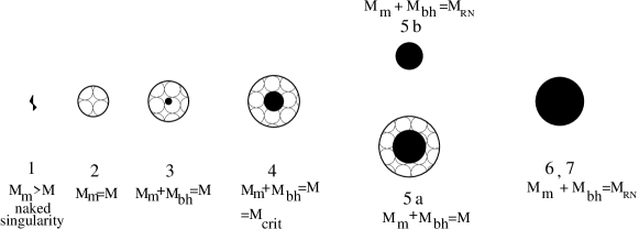
Figure 2: The space of solutions in a $M_{\rm m}\times M$, where $M=M_{\rm m}+M_{\rm bh}$ is the total mass, is plotted (see also leenairweinbergPRD92 ). For each point 1-7, along a constant monopole mass, in the diagram, the corresponding configuration is pictorially represented in the bottom part of the figure.

Figure 3: The space of solutions in a $a\times r_{\rm bh}$ diagram (see also breitenetal1 ).

To understand the generic behavior it is helpful to make a plot of the solution space. One such plot is given in a $M_{\rm m}\times M$, where $M=M_{\rm m}+M_{\rm bh}$ is the total mass. This is shown in Figure 2, see also leenairweinbergPRD92 . There are four areas and three lines. The pure monopole line, (the regular solutions discussed above) with the total mass equal to the monopole mass, is represented by a line with slope 1. The top-left region represents naked singularities. The center-left area represents monopole+Schwarzschild (non-Abelian) black hole solutions mentioned above. At arbitrarily near the critical mass the solutions are extremal magnetic charged Reissner-Nordström quasi-black holes (and at precisely the critical mass they turn into degenerated solutions). To the right there is a region where monopole+Schwarzschild (non-Abelian) black holes coexist with magnetic (Abelian) Reissner-Nordström black holes. Then to the far right and above there is a region of magnetic (Abelian) Reissner-Nordström black holes alone. In this diagram, solutions with a constant black hole mass are represented by lines parallel to the pure monopole line, i.e., lines of slope 1. Lines of constant monopole mass are horizontal lines. We show pictorially each representative configuration along a constant monopole mass line. Each numbered point (from 1 to 7) in Figure 2 is represented in the bottom of the figure by a schematic drawing. In this drawing, note that the horizon area of the solution containing a Schwarzschild black hole surrounded by monopole matter (numbered 5a) is larger than the horizon area of the pure magnetic Reissner-Nordström horizon (numbered 5b). Following the area law, the smaller one is prone to be unstable and decay to the larger hairy one. This has interesting implications in the ultimate fate of the black hole through Hawking evaporation leenairweinbergPRL92 .

Another similar but interesting plot is $a\times r_{\rm bh}$ diagram, shown in Figure 3, see also breitenetal1 . There are four areas and four lines. There is the pure monopole line ($r_{\rm bh}=0$), which yields the regular solutions discussed above. The top-left area is the region of no solutions. There is the center-left area of monopole+Schwarzschild (non-Abelian) black hole solutions discussed above, there is the bottom-left area where one finds monopole+Schwarzschild (or non-Abelian) black hole solutions as well as magnetic (Abelian) Reissner-Nordström black holes, and then the right area of magnetic (Abelian) Reissner-Nordström black holes. The other lines are boundaries between these areas.

II.3 The gravitational behavior as a function of $a$ (gravitation) for high $b$ (high Higgs mass)

High Higgs mass reserves surprises. Here we overview the solutions found in lueweinberg1 ; lueweinberg2 still keeping in mind that we will later need them for comparison. High $b$ means $b\buildrel>\over{\sim}40$ lueweinberg1 . From subsection IIA, high $b$ indicates a large Higgs mass $m_{\rm H}$, or small associated Compton wavelength. This means that the Higgs field does participate in the dynamics, and can have great influence on the monopole structure. Reinterpreted through Equation (13) one can also see high $b$ as a monopole with large secondary mass $M_{\rm m_{2}}$, or small secondary radius $r_{\rm m_{2}}$. In order to understand how the structure changes as gravity is turned on higher and higher one has to increase the parameter $a$.

II.3.1 The regular magnetic monopole solution: from no gravitation to the extremal black hole

For low $a$ there is not much change in relation to the low $b$ case. Low $a$ represents a highly dispersed magnetic monopole, with small mass $M_{\rm m}$ and large radius $r_{\rm m}$. As $a$ increases the solution gets more general relativistic and eventually gets to a black hole, when $a=a_{\rm crit}\sim 1$. An important difference to the low $b$ case is that instead of passing from a quasi-horizon to a degenerate spacetime, it passes from a quasi-horizon to a true horizon, well inside the core at $r_{*_{2}}$ lueweinberg2 . To get a grip on the solutions we draw in Figure 4 diagrams showing the metric functions and the matter field functions as a function of $r$ for two values of $a$, $a$ small and $a_{\rm crit}$. Specifically the behavior of the functions is: (i) The function $1/A$, the metric function that signals the formation of a black hole, shows that very near $a_{\rm crit}$ there are two radial scales, where horizon could be formed, one at $r_{*_{2}}$ (related to the scale set by the Higgs mass), the other at $r=r_{*}$ (related to the scale set by the the W mass), but at $a_{\rm crit}$ the double zero occurs at $r_{r*_{2}}$, and an extremal horizon appears there. (ii) The metric function $B$ shows also a zero at $r_{*_{2}}$ signaling the formation of an infinite redshift surface. Note now that $B$ is zero at one point only, $r_{r*_{2}}$, not in a whole region as was the case for low $b$. This means that the configuration quasi-black hole with radius very near $r_{*_{2}}$, turns into a true extremal black hole rather than to a degenerate spacetime as in the low $b$ case. (iii) The behavior of $(AB)^{1/2}$, which tells whether the horizon is naked or not, confirms this behavior. It shows that it is never zero, meaning the horizon is a regular, not a naked one lueweinberg2 . This means that the components of the Riemann tensor at the horizon in an orthonormal frame are well behaved. In this case a particle that is sent in through the monopole, turns around, and comes back to the point where it started, takes a proper time $\Delta\,\tau$ which is finite, non-zero. Thus, since the Riemann tensor is proportional to $(\Delta\,\tau)^{-2}$, as discussed in connection to the low $b$ case, there is no funny behavior at the horizon and all behaves well. (iv) The function $u$ for the Yang-Mills field shows that for $a_{\rm crit}$ there is field outside the horizon radius, i.e., there is hair. (v) The function $h$ for the Higgs field, behaves similarly to $u$. In the critical situation, it only acquires the vacuum value for radii much larger than $r_{*_{2}}$.

Figure 4: The graphs of the metric and matter functions, $(1/A,B,(AB)^{1/2},u,h)$, are plotted as a function of $r$ in the high $b$ case. The curves $a$ small are typical of small gravitational effects, and the curves $a$ critical give the properties of the extremal quasi-black hole. The radius $r_{*}$ is the the radius at which the quasi-horizon is formed, see text for details.

There are three points that are worth commenting. First, we comment further on the behavior of $(AB)^{1/2}$ and its consequences. In terms of the coordinate time, the particle takes for the round trip the time $\Delta t\sim r_{*_{2}}\,\epsilon^{-1/2}$, where again $\epsilon\equiv(1/A)_{\rm min}$ is a very small number. Thus the particle takes, as in the low $b$ case, a long time to return to a coordinate observer, and this is important in connection with entropy issues lueweinberg2 . Indeed, in leading order, this time is determined only from the spacetime geometry. An observer finds that the quasi-black hole has an inside which is inaccessible, since probes stay there for an arbitrarily large amount of time, and describes it by a density matrix $\rho_{\rm matrix}$ obtained by tracing over the degrees of freedom inside the quasi-horizon, yielding an entropy $S=-\,{\rm Tr}\left(\,\rho_{\rm matrix}\,\ln\rho_{\rm matrix}\right)$. The calculation of the interior entropy of a field inside a spherical box was performed for a scalar field with the result that $S=\gamma\frac{A}{4}$, where $\gamma$ is an undetermined factor, and $A$ is the area of the box srednicki . In this case, the box is the magnetic monopole quasi-horizon configuration on the verge of being a black hole. Since one can give a little push from this configuration to the horizon configuration, and in the latter case the entropy is $S=\frac{A}{4}$ one can guess by continuity that the coefficient of proportionality in the quasi-horizon case has a dependence on the size of the box $\gamma=\gamma(r_{\rm box})$ and when a horizon forms, $\gamma(r_{*_{2}})=\frac{1}{4}$ lueweinberg2 . In this sense, the entropy of the extremal black hole is the number of the entangled degrees of freedom inside the horizon. This analysis cannot be applied to the low $b$ case because there is never a true horizon: in the limit, when the object is turning into a black hole it gives a non-smooth manifold.

Second, another feature of these monopoles is that they have a charge to mass ratio given by $Q/M>1$. Thus if one drops neutral matter onto a regular magnetic monopole one can form an extremal black hole lueweinberg2 . This is contrary to the case of electric Reissner-Nordström black holes with $Q/M<1$, and where one can drop charged matter, with charge $q$ and mass $m$ obeying $q/m>1$, as much as one wants that one never gets an extremal black hole (this is a version of the third law of black hole mechanics).

Third, one can ask what happens for $a$ higher than the critical value. Following lueweinberg2 one finds that there are possibly two branches. One branch is formed of magnetically Abelian charged Reissner-Nordström black holes. The other branch, has non-Abelian matter and hair outside, a horizon, and regular non-Abelian matter inside. Following theorems by Borde borde ; beato1 ; beato2 one finds that these regular solutions may have different inside and outside topologies. This issue should be further explored.

II.3.2 The Schwarzschild black hole solution inside the monopole

As in the low $b$ case one can put a Schwarzschild black hole inside. This was done in brihaye1 . The main feature is that again there is hair outside the true horizon. The results are in line with what we have been discussing. Diagrams like those of Figures 2 and 3 can be drawn, although we have not found them in the literature.

II.4 Further discussion

Thus, gravitationally there are two distinct behaviors, the low $b$ case and the high $b$ case, the marginal case being at $b\simeq 40$. The low $b$ case has the following main features: when one turns on gravitation (when one increases $a$) a quasi-black hole appears from the regular monopole, which turns into a degenerate spacetime at the critical value $a_{\rm crit}$; it has a naked horizon, and shows no hair, i.e., it is of Coulumb type, the non-trivial fields are hidden inside the horizon. In addition, one can enrich the monopole structure by putting a Schwarzschild black hole inside up to a certain maximum mass. The high $b$ case has also a regular monopole solution which, when one increases the gravitational parameter $a$, turns into a quasi-black hole, and then at $a_{\rm crit}$ a true extremal black hole appears, with regular horizon and hair. There is a transition between the two cases, a first order type transition. When $b$ is in the transition zone, there is a double double zero, one zero at $r_{*}$ and the other at $r_{*_{2}}$. So, the transition is discontinuous in radius, and thus in entropy. It is, however, continuous in mass lueweinberg1 .

Other features that are also very interesting but not important in our context are: (i) For very low $b$ ($b<0.1$, say), the behavior is more complicated near $a_{\rm crit}$ breitenetal1 . If one increases $a$ from zero, one passes $a_{\rm crit}$ up to an $a_{\rm max}$. But from $a_{\rm crit}$ to $a_{\rm max}$ there are two solutions, one with larger mass $M_{\rm m}$ (larger radius $r_{\rm m}$), the other with smaller values. The one with smaller values is the one that connects continuously with the low mass solutions. The smaller mass solutions are stable, and so the branch which forms black holes is unstable; (ii) For a certain range of the parameters $a$ and $b$, there are multiple node solutions (nodes appearing in the function $u(r)$ of the Yang-Mills field) of the type found in the Bartnick-Mckinonn solution breitenetal1 ; (iii) The particular case $b\rightarrow\infty$ in the high $b$ sector was analyzed in detail by Aichelburg and Bizon bizon . The solution has a conical singularity at $r=0$ but apart from that it is well-behaved. Perhaps, oddly, core behavior in this limit was not found, we will comment on this later on.

This program of studying the gravitational behavior of magnetic monopoles has been continued by Brihaye et al, where the structure of dyonic non-Abelian black holes has been analyzed brihaye2 ; brihaye3 , and gravitational monopoles in $SU(3)$, $SU(5)$, and $SU(N)$ theories have been found brihaye4 ; brihaye5 ; brihayeN .

III Gravitational behavior of Majumdar-Papapetrou matter systems: two concentric spherical thin shells

III.1 The Majumdar-Papapetrou sector of the Einstein$-$Maxwell-charged dust system

III.1.1 The action and equations of motion

We now want to study the Einstein-Maxwell system coupled to some specific electrically charged dust currents as will be described below. By dust one means a fluid with zero pressure. We will compare the configurations found below with the magnetic configurations discussed in section II. A first study in this direction has been done in lemosweinberg (see also kleberlemoszanchin ). The action for the Einstein$-$Maxwell-charged dust system is $(G=c=1)$

$$S=\int d^{4}x\sqrt{-g}\left(\frac{1}{16\,\pi}R+{\cal L}_{\rm matter}\right)\,,$$ (15)

where $R$ is the scalar curvature, and

$${\cal L}_{\rm matter}={\cal L}_{\rm Maxwell}+{\cal L}_{\rm charged\,dust}+{\cal L}_{\rm int}\,.$$ (16)

The Maxwell Lagrangian is

$${\cal L}_{\rm Maxwell}=-\frac{1}{4}F_{\mu\nu}F^{\mu\nu}\,,$$ (17)

$$F_{\mu\nu}=\partial_{\mu}A_{\nu}-\partial_{\nu}A_{\mu}\,,$$ (18)

where $F_{\mu\nu}$ and $A_{\nu}$ are the electromagnetic field strength and potential, respectively. The charged dust Lagrangian, ${\cal L}_{\rm charged\,dust}$, is such that the action integral, $S_{\rm dust}=\int d^{4}x\,\sqrt{-g}\,{\cal L}_{\rm dust}$, gives the energy-momentum tensor for charged dust, i.e.,

$$T_{\rm charged\,dust}^{\mu\nu}=-\frac{1}{8\pi}\,\frac{1}{\sqrt{-g}}\frac{\delta S_{\rm charged\,dust},}{\delta\,g^{\mu\nu}}=\rho\,u^{\mu}\,u^{\nu}\,,$$ (19)

where $\rho$ is the dust energy density and $u^{\mu}$ its four-velocity. The interaction Lagrangian ${\cal L}_{\rm interaction}$ is given by

$${\cal L}_{\rm interaction}=A_{\mu}\,j^{\mu}\,,$$ (20)

where $j^{\mu}=\rho_{\rm e}\,u^{\mu}$, $\rho_{\rm e}$ being the electric charge density. The elementary particles are then the electromagnetic massless photon, the massless graviton, and the massive charged dust particles with energy density $\rho$ and charge density $\rho_{\rm e}$. The charged dust particles may spread over a given three-dimensional region of space, or can be squeezed into a two-dimensional thin membrane, i.e., a shell. In the latter case the action (15) acquires the form of a bulk action plus a membrane action. These bulk plus membrane systems will be treated now.

The configuration we want to discuss is spherically symmetric, a star type configuration, with metric given again by

$$ds^{2}=-B(r)\,dt^{2}+A(r)\,dr^{2}+r^{2}\left(d\theta^{2}+\sin^{2}\theta\,d\phi^{2}\right)\,,$$ (21)

and with the electric Maxwell field given by

$$A_{0}=\varphi(r)\,,\quad A_{i}=0\,.$$ (22)

Putting this ansatz into the Einstein$-$Maxwell-charged dust action (15) and varying the action with relation to the three functions, yields three equations, two for the gravitational field $B(r)$ and $A(r)$, and one for the Maxwell field $\varphi(r)$. The equations are, respectively,

$$\frac{(AB)^{\prime}}{AB}=8\pi\,r\,\rho\,A\,,$$ (23)

$$\left[r\left(1-\frac{1}{A}\right)\right]^{\prime}=8\pi\,r^{2}\,\rho+\frac{r}{A\,B}\,\varphi^{\prime 2}\,,$$ (24)

$$\frac{\sqrt{B}}{r^{2}\sqrt{AB}}\left[\frac{r^{2}}{\sqrt{AB}}\,\varphi^{\prime}\right]^{\prime}=-4\pi\rho_{\rm e}\,.$$ (25)

There are three parameters in the theory: $G$ which we have set equal to one, $\rho$ and $\rho_{\rm e}$. Now, $\rho$ and $\rho_{\rm e}$ have dimensions of length to minus two. Thus one can form in principle two length scales. The ratio of these length scales yields a parameter without dimensions. One particular class of solutions, the one we want to treat, sets

$$\frac{\rho_{\rm e}}{\rho}=1\,.$$ (26)

(Note that the charge density $\rho_{\rm e}$ can have two signs, so strictly speaking one should put $\rho_{\rm e}=\pm\rho$. In order to not carry this $\pm$ throughout we drop the minus sign, bearing in mind that a $-$ sign can be floating about.) Matter obeying the condition (26), i.e., matter with mass equal to charge, can be called extremal charged dust in analogy with the extremal Reissner-Nordström black holes. The system of equations (23)-(25) with condition (26) is the the Majumdar-Papapetrou system majumdar ; papapetrou .

Now, in order to show a behavior analogous to the magnetic monopole of the Einstein$-$Yang-Mills$-$Higgs system the Majumdar-Papapetrou system per se is not enough, the parameters do not give enough structure. In order to get more structure we have to add new parameters. First assume a given spherical symmetric solution, which we call a star. Then, a new parameter is the radius of the star, $r_{\rm star}$. So now, one has two parameters $\rho$ and $r_{\rm star}$. It is preferable to swap the star’s density $\rho$ for the star’s mass $M_{\rm star}$, so that the two parameters are $M_{\rm star}$ and $r_{\rm star}$. Then one can form an adimensional parameter

$$a=\frac{M_{\rm star}}{r_{\rm star}}\,.$$ (27)

This is the equivalent to the parameter $a$ in the Einstein$-$Yang-Mills$-$Higgs theory, see (12). To simplify the analysis, and without loss of generality, we can think that the star is made of a thin shell of extremal charged dust, with $M_{\rm star}$ and $r_{\rm star}$ being now the mass and the radius of the thin shell. It is not difficult to see that this thin shell is a solution of the Majumdar-Papapetrou system kleberlemoszanchin . One can now further bring into the problem a new extremal charged thin shell, called the secondary shell, with two new parameters, the mass $M_{2}$ and the radius $r_{2}$. One has then two thin shells, one inside the other, a configuration that is also a solution of the Majumdar-Papapetrou system, as will be displayed below. One can then form a new dimensionless parameter $b$ given by

$$b=\frac{M_{2}/r_{2}}{M_{\rm star}/r_{\rm star}}\,.$$ (28)

This is equivalent to the secondary parameter of the Einstein$-$Yang-Mills$-$Higgs system appearing in equation (13). This double shell solution has four parameters $M_{\rm star},r_{\rm star},M_{2},r_{2}$. In order to produce the required model one should restrict these four parameters through a constraint equation, as in the magnetic monopole case. Generically, the two shells are indistinguishable, one cannot say whether the outer one is the star or the secondary shell. To be definitive, the inner shell it is called the secondary shelll, the outer shell is the star, and we keep the secondary shell always inside the star, through the constraint

$$r_{\rm star}=2\,r_{2}\,.$$ (29)

The factor $2$ in (29) was chosen for convenience, any real number greater than one will do. Equation (29) is the equivalent to the constraint (14) in the magnetic monopole case. Thus the system we are going to work with is a Majumdar-Papapetrou system with two extremal charged shells. This simple system mimics a good deal of behavior of the Einstein$-$Yang-Mills$-$Higgs system. Instead of working with thin shells, one could work with the thick shell solutions found in kleberlemoszanchin or with the Bonnor stars bonnor2 ; bonnor3 ; bonnor4 , but this only complicates the technical analysis of the problem without further illuminating it.

III.1.2 Some properties and scales of the Majumdar-Papapetrou double shell

We are now ready to put a shell within a shell, and simulate the behavior of the gravitational magnetic monopoles. The star (outer shell) and the secondary shell (inner shell) are considered to be infinitesimally thin, see Figure 5. Then, the metric valid from $0\leq r<\infty$, for a Majumdar-Papapetrou spacetime with two extremal matter thin shells, is given by

$$ds^{2}=-\frac{\left(1-\frac{M}{r_{\rm star}}\right)^{2}\left(1-\frac{M_{2}}{r_{2}}\right)^{2}}{\left(1-\frac{M_{2}}{r_{\rm star}}\right)^{2}}\,dt^{2}+dr^{2}+r^{2}\left(d\theta^{2}+\sin^{2}\theta\,d\phi^{2}\right)\,,\quad 0\leq r\leq r_{2}\,,$$ (30)

$$ds^{2}=-\frac{\left(1-\frac{M}{r_{\rm star}}\right)^{2}}{\left(1-\frac{M_{2}}{r_{\rm star}}\right)^{2}}\left(1-\frac{M_{2}}{r}\right)^{2}\,dt^{2}+\frac{dr^{2}}{\left(1-\frac{M_{2}}{r}\right)^{2}}+r^{2}\left(d\theta^{2}+\sin^{2}\theta\,d\phi^{2}\right)\,,\quad r_{2}\leq r\leq r_{\rm star}\,,$$ (31)

$$ds^{2}=-\left(1-\frac{M}{r}\right)^{2}\,dt^{2}+\frac{dr^{2}}{\left(1-\frac{M}{r}\right)^{2}}+r^{2}\left(d\theta^{2}+\sin^{2}\theta\,d\phi^{2}\right)\,,\quad r_{\rm star}\leq r<\infty\,,$$ (32)

where $M=M_{\rm star}+M_{2}$ is the total mass of the system. The constants in the $g_{tt}$ components were chosen so that the metric matches at the shells. The electric field is

$$\varphi=1-\frac{\left(1-\frac{M}{r_{\rm star}}\right)\left(1-\frac{M_{2}}{r_{2}}\right)}{\left(1-\frac{M_{2}}{r_{\rm star}}\right)}\,,\quad 0\leq r\leq r_{2}\,,$$ (33)

$$\varphi=1-\frac{\left(1-\frac{M}{r_{\rm star}}\right)\left(1-\frac{M_{2}}{r}\right)}{\left(1-\frac{M_{2}}{r_{\rm star}}\right)}\,,\quad r_{2}\leq r\leq r_{\rm star}\,,$$ (34)

$$\varphi=1-\left(1-\frac{M}{r}\right)=\frac{M}{r}\,,\quad r_{\rm star}\leq r<\infty\,.$$ (35)

The fluid field is given by the surface energy densities of the shells. For the secondary thin shell one has that the surface energy density $\sigma_{2}$ is given by

$$\sigma_{2}=\frac{M_{2}}{4\pi r_{2}^{2}}\,,$$ (36)

with the the corresponding surface electric charge density of the shell $\sigma_{{\rm e}_{2}}$ given by $\sigma_{{\rm e}_{2}}=\sigma_{2}$. For the thin shell star one has that the surface energy density $\sigma_{\rm star}$ is given by

$$\sigma_{\rm star}=\frac{M_{\rm star}}{4\pi r_{\rm star}^{2}}\,,$$ (37)

with the corresponding surface electric charge density of the shell $\sigma_{{\rm e}_{\rm star}}$ given by $\sigma_{{\rm e}_{\rm star}}=\sigma_{\rm star}$. Note that the $g_{rr}$ component of the metric has a step function at $r_{2}$ and $r_{\rm star}$. This is no problem, one can smooth it out by considering a shell with small thickness kleberlemoszanchin , but for the problem we are considering it is irrelevant.

Figure 5: A schematic drawing of the double shell solution in the Majumdar-Papapetrou system, showing the secondary shell inside the star shell.

One important question is which shell, and in which conditions a shell, forms a horizon. We know that a horizon should form when $1/A=0$. Suppose a $b$ is given, and one starts to increase $a$. Then it is meaningfull to ask which shell forms first a horizon, the star or the secondary shell? To answer it note that

$$\left.\frac{1}{A}\right)_{r_{2}}=1-\frac{M_{2}}{r_{2}}=1-ab\,,$$ (38)

$$\left.\frac{1}{A}\right)_{r_{\rm star}}=1-\frac{M}{r_{\rm start}}=1-\frac{M_{\rm star}}{r_{\rm star}}\left(1+\frac{M_{2}/r_{2}}{M_{\rm star}/r_{\rm star}}\frac{r_{2}}{r_{\rm star}}\right)=1-a\left(1+\frac{b}{2}\right)\,.$$ (39)

It is then clear that there are three cases:

$b<2$ $-$

when $a$ increases an external horizon forms first at $r_{\rm star}=M$, with $a_{\rm crit}=1/(1+b/2)$. This is analogous to the behavior of magnetic monopoles with low $b$, where an external horizon forms outside the core.

$b>2$ $-$

when $a$ increases an interior horizon forms first at $r_{2}=M_{2}$, with $a_{\rm crit}=\frac{1}{b}$. This is analogous to behavior of magnetic monopoles with high $b$, where an external horizon forms within the core.

$b=2$ $-$

when $a$ increases a horizon forms at both shells, interior and exterior with $a_{\rm crit}=1/2$. This divides the two cases above.

As we will show below the solution does not develop a true horizon. Independently of $b$, upon increasing $a$, a quasi-horizon appears. Then at the critical value one gets a degenerated spacetime, and for values of $a$ above the critical there is no static solution, the shell collapses (see gaolemos ) into a singularity and an extremal Reissner-Norström black hole forms. In what follows we study each type of configuration. We start with low $b$, $b<2$, then we do high $b$, $b>2$.

III.2 The gravitational behavior as a function of $a$ for low $b$

Since $b=\frac{M_{2}/r_{2}}{M_{\rm star}/r_{\rm star}}$, low $b$ can be seen as a relatively small secondary mass $M_{2}$, or large secondary radius $r_{2}$, which means that the secondary shell has little influence in the structure. Given a low $b$ configuration, we want to understand how the structure changes as the parameter $a=\frac{M_{\rm star}}{r_{\rm star}}$ increases. We present plots giving the behavior of the metric and matter functions as a function of radius for typical cases, discuss the naked horizon behavior and the Coulumb character of these solutions, put an extremal Reissner-Nordström black hole inside, and sketch some diagrams covering the space of solutions.

III.2.1 The regular Majumdar-Papapetrou double shell solution: from no gravitation to the extremal quasi-black hole and beyond

We have seen from Equations (38)-(39) that for fixed $b$, with $b<2$, an extremal quasi-horizon appears when the parameter $a$ increases, i.e., when one puts more gravitation into the star shell. A small $a$ parameter, i.e., $M_{\rm star}/r_{\rm star}$ small, means that the star shell is very dispersed. As $a$ increases, eventually it gets to a stage where a kind of an extremal event horizon forms. Using Equations (30)–(39) one can plot the behavior of the metric and matter functions as a function of radius for two values of $a$, $a$ small, and $a$ arbitrarily near $a_{\rm crit}$, when a quasi-horizon forms, see Figure 6. Specifically, the behavior of the functions $1/A$, $B$, $(AB)^{1/2}$, $\varphi$, and $\sigma$ is: (i) The function $1/A$ signals the formation of a black hole. For $a$ small the function $1/A$ starts at the value 1 (thus there are no conical singularities) drops slightly at the secondary shell, rises and drops again at the star shell, and then rises again to 1 at infinity. When $a=a_{\rm crit}$ (or arbitrarily near it) the function gets a ‘double’ zero at $r=r_{*}$ (it would be a double zero had we smoothed out enough the matter) signaling the formation of a kind of an extremal Reissner-Nordström black hole. (ii) The function $B$, the redshift function, has the usual behavior for $a$ small. However, for $a_{\rm crit}$ the whole of the region inside $r_{*}$ gets infinitely redshifted. This means that the manifold is not smooth. Thus the critical case is not a true black hole, it is a degenerated spacetime. (iii) The product function $(AB)^{1/2}$ is important to determine whether the forming horizon is naked or not. We find that a particle on a return trip to the star takes a proper time given by $\Delta\tau\sim r_{*}\,\epsilon^{1/2}$, where $r_{*}$ is the radius of the quasi-horizon, and, near the critical solution, $\epsilon\equiv(1/A)_{\rm min}$ is a very small quantity kleberlemoszanchin . Since this proper time is arbitrarily small, the Riemann tensor diverges at the horizon, and the horizon is naked. For completeness we give the coordinate time $\Delta t$ taken by the particle in its trip, $\Delta t\sim r_{*}\,\epsilon^{-1/2}$, implying that the particle takes a long time to return for a coordinate observer. (iv) The function $\varphi$ tells whether the solution has hair or not. It starts constant, then decays with $1/r$, with a bump at $r_{2}$ and at $r_{\rm star}$. When the horizon forms the field is a pure Coulumb field, showing no-hair. (v) The surface density function $\sigma$ of the charged dust is also drawn, for completeness. Outside the quasi-horizon at $r_{*}$ there is no matter.

Figure 6: The graphs of the metric and matter functions, $(1/A,B,(AB)^{1/2},\varphi,\sigma)$, are plotted as a function of $r$ in the low $b$ ($b<2$) case. The curves $a$ small (dashed lines) are typical of small gravitational effects, and the curves $a$ critical (full lines) give the properties of the extremal electrical quasi-black hole. The radius $r_{*}$ is $r_{\rm star}$ at the quasi-horizon (arbitrarily near the critical radius), see text for details. (In the graphs, we have used $b=1$ as a typical low $b$ case, and have set $M_{\rm star}=\frac{5}{2}$, $M_{2}=\frac{5}{4}$, and for $a$ small we have put $r_{\rm star}=10$, $r_{2}=5$, while for $a$ critical we have put $r_{\rm star}=\frac{15}{4}$, $r_{2}=\frac{15}{8}$.)

The case $b=0$ is worth discussing because it is the simplest one in the low $b$ sector. There is no secondary shell ($M_{2}=0$) and so it represents a single thin shell with mass $M_{\rm star}$ and radius $r_{\rm star}$. It is interesting because on one hand it has the same properties of any other low $b$ case, on the other hand, it is easier to figure out what happens above criticality, i.e., for $a>a_{\rm crit}$ ($M_{\rm star}>r_{\rm star}$). We have seen that when the precise equality holds, $a=a_{\rm crit}$, the redshift function $B$ is zero not only at the horizon but also in the whole region inside, meaning that in fact a true black hole does not form, since inside there is no smooth manifold. For $a>a_{\rm crit}$ one seems to have now a shell of matter at $r_{\rm star}$ inside an extremal electrical Reissner-Nordström black hole at $r_{\rm bh}=M_{\rm star}$, the solution being everywhere free from curvature singularities. Following a theorem by Borde borde , this would mean that the topology of spacelike slices in this black hole spacetime would change from a region where they are noncompact to a region where they are compact, in the interior. In our case this in fact does not happen, there are no solutions with $a>a_{\rm crit}$, i.e., $m>r_{\rm o}$, the shell collapses into a singularity gaolemos .

III.2.2 Non-regular Majumdar-Papapetrou shell solutions: The extremal Reissner-Nordström black hole solution inside the thin shell star

One can put a black hole inside the double thin shell and obtain a structure similar to the one found when one puts a black hole inside a magnetic monopole. For the double thin shell, the extra inner black hole has to be an extremal Reissner-Nordström black hole, rather than a Schwarzschild black hole, to keep the solutions within the Majumdar-Papapetrou system. If one puts a non-extremal black hole foreign tensions would develop at the thin shells. So, in order to stick to pure Majumdar-Papapetrou system we stick to an inner extremal Reissner-Nordström black hole. In order to simplify the analysis, we will work with the $b=0$ which is a good simple case for low $b$. For any other small $b$, such that $b<2$, the result is analogous. In the $b=0$ case one has $M_{2}=0$. Thus the system is formed by the star shell with mass $M_{\rm star}$ and radius $r_{\rm star}$, and an inner extremal Reissner-Nordström black hole with mass $M_{\rm bh}$ and radius $r_{\rm bh}$ ($M_{\rm bh}=r_{\rm bh}$). The metric is now

$$ds^{2} = -\left(1-\frac{M_{\rm bh}}{r}\right)^{2}\frac{\left(1-\frac{M}{r_{\rm star}}\right)^{2}}{\left(1-\frac{M_{\rm bh}}{r_{\rm star}}\right)^{2}}\,dt^{2}+\frac{dr^{2}}{\left(1-\frac{M_{\rm bh}}{r}\right)^{2}}+$$ (40)

$$r^{2}\left(d\theta^{2}+\sin^{2}\theta\,d\phi^{2}\right)\,,\quad 0\leq r\leq r_{\rm star}\,,$$

$$ds^{2}=-\left(1-\frac{M}{r}\right)^{2}\,dt^{2}+\frac{dr^{2}}{\left(1-\frac{M}{r}\right)^{2}}+r^{2}\left(d\theta^{2}+\sin^{2}\theta\,d\phi^{2}\right)\,,\quad r_{\rm star}\leq r\,,$$ (41)

where here $M=M_{\rm star}+M_{\rm bh}$ is now the total mass. The electric field $\varphi(r)$ and the charge density field $\rho(r)=\sigma_{\rm star}(r_{\rm star})$ profile accordingly.

Figure 7: The space of solutions in a $M_{\rm star}\times M$, where $M=M_{\rm star}+M_{\rm bh}$ is the total mass, is plotted. For each point 1-5, along a constant star mass, in the diagram, the corresponding configuration is pictorially represented in the bottom part of the figure. This is the graph made in Figure 2 (see also leenairweinbergPRD92 ) adapted to the thin shell Majumdar-Papapetrou system.

Figure 8: The space of solutions in an $a\times r_{\rm bh}$ plot, where $a=\frac{M_{\rm star}}{r_{\rm star}}$, and $r_{\rm bh}$ is the radius of the Reissner-Nordström black hole inside the star. This is the graph drawn in Figure 3 (see also breitenetal1 ) adapted to the thin shell Majumdar-Papapetrou system.

To understand the generic behavior of this system it is helpful to make a plot of the solution space, similar to the plot made for a Schwarzschild black hole inside the magnetic monopole shown in Figure 2. We do this in Figure 7, where we plot the solution space in a $M_{\rm star}\times M$ diagram for fixed $r_{\rm star}$. There are three regions and two lines. The pure star line, i.e., the regular solutions discussed above with the total mass equal to the star mass, is represented by a line with slope 1. The top-left region represents extremal charged naked singularities. The center-left region represents star+(extremal Reissner-Nordström black hole) solutions displayed in Equations (40)-(41). At values arbitrarily near the critical mass $M_{\rm crit}$ the solutions are extremal electric charged Reissner-Nordström quasi-black holes, which degenerate at the critical value. To the right there is a region of a totally collapsed shell star inside an extremal Reissner-Nordström black hole, which means the solutions represent pure extremal Reissner-Nordström black holes. We show pictorially each representative configuration along a constant star mass line. Each numbered point (from 1 to 5) in Figure 7 is represented in the bottom of the figure by a schematic drawing. We see that taking $M_{\rm star}$ constant and increasing $M$ we pass through point 1 where $M_{\rm star}$ is greater than $M$ and therefore there is a negative mass at the center, through point 2 where one finds a thin shell solution with $M_{\rm star}=M$, through point 3 where there is a black hole inside the star, through point 4 which is the case arbitrarily near the critical value where $M_{\rm star}+M_{\rm bh}=r_{\rm star}$, and thus an extremal quasi-black hole appears at $r_{\rm star}$, finally to point 5 where $r_{\rm star}$ has collapsed inside the horizon radius to form an extremal black hole. Note there is a jump in horizon radius from a point infinitesimally to the left of point 4, to a point infinitesimally to the right of point 4. Note also that this diagram is done for fixed $r_{\rm star}$. For another value of $r_{\rm star}$, one gets the same diagram, but with the vertical critical line critical shifted, to the right when the new $r_{\rm star}$ is larger, and to the left when the new $r_{\rm star}$ is smaller than the original value. Comparison of the Figures 2 and 7 shows the similarities between the magnetic monopole and the Majumdar-Papapetrou system.

One can also translate Figure 3 into this Majumdar-Papapetrou system. This is done in Figure 8, where we display the important regions in a graph $a\times r_{\rm bh}$, where again $a=\frac{M_{\rm star}}{r_{\rm star}}$, and $r_{\rm bh}$ is the radius of the Reissner-Nordström black hole inside the star. There are two regions and two lines. There is the vertical line, $r_{\rm bh}=0$, of regular star solutions. There is the region where star+(extremal electric Reissner-Nordström black hole) solutions exist. There is the line where the system forms a quasi-black hole (i.e., a solution arbitrarily near the critical degenerate case). Finally there is the region where an extremal electric black hole exists. The naked singularity region, not shown, would appear for negative $r_{\rm bh}$, i.e., for negative black hole masses, $r_{\rm bh}=M_{\rm bh}<0$.

III.3 The gravitational behavior as a function of $a$ for high $b$

High $b$ can be seen as a relatively large secondary mass $M_{2}$, or small secondary radius $r_{2}$, which means that the secondary shell has a decisive influence in the structure. Given a high $b$ configuration, we want to understand how the structure changes as the parameter $a=\frac{M_{\rm star}}{r_{\rm star}}$ increases. We present plots giving the behavior of the metric and matter functions as a function of radius for typical cases, discuss the naked horizon behavior and the non-Coulumb character of these solutions, and we briefly comment on putting an extremal Reissner-Nordström black hole inside the high $b$ double shell system.

III.3.1 The regular solution: from no gravitation to the extremal quasi-black hole and beyond

Figure 9: The graphs of the metric and matter functions, $(1/A,B,(AB)^{1/2},\varphi,\sigma)$, are plotted as a function of $r$ in the high $b$ ($b>2$) case. The curves $a$ small (dashed lines) are typical of small gravitational effects, and the curves $a$ critical (full lines) give the properties of the extremal quasi-black hole. The radius $r_{*}$ is now $r_{2}$ at the quasi-horizon, see text for details. (In the graphs, we have used $b=4$ as a typical high $b$ case, and have set $M_{\rm star}=\frac{5}{4}$, $M_{2}=\frac{5}{2}$, and for $a$ small we have put $r_{\rm star}=10$, $r_{2}=5$, while for $a$ critical we have put $r_{\rm star}=5$, $r_{2}=\frac{5}{2}$.)

In contrast with low $b$, in the high $b$ case, an extremal quasi-horizon forms at the secondary shell $r_{2}$, rather than in the star shell. Using Equations (30)–(39) one can draw the important field functions as a function of $r$, for a given high $b$ and for two values of $a$, $a$ small and $a$ critical, see Figure 9. The behavior of the functions $1/A$, $B$, $(AB)^{1/2}$, $\varphi$, and $\sigma$ is: (i) For $a$ small the function $1/A$ starts at the value 1 drops at the secondary shell, rises and drops slightly at the star shell, and then rises again to 1 at infinity. When $a$ is arbitrarily near $a_{\rm crit}$ the function gets a double zero at $r=r_{*}$, now situated at the secondary shell $r_{2}$, signaling the formation of a quasi-horizon. (ii) For $a$ small, the function $B$ has the usual behavior. For $a$ arbitrarily near $a_{\rm crit}$, $B$ is arbitrarily near zero throughout the region inside $r_{2}$. At $a=a_{\rm crit}$ precisely the manifold is not smooth. Thus again, the critical case is not a true black hole, it is a degenerate manifold. (iii) The function $(AB)^{1/2}$ is zero inside the quasi-horizon confirming the existence of a naked behavior. This is not quite the same as the high $b$ behavior for the magnetic monopole, since the magnetic system gets in the high $b$ case a non-naked horizon. (iv) At $a$ arbitrarily near $a_{\rm crit}$, the function $\varphi$ does not have a Coulumb type behavior as one can see from Figure 9, the elctric field outside the quasi-horizon gets a bump due to the presence of the outer shell. Strictly speaking one cannot talk of a no-hair violation since the no-hair theorem is applied to black holes, not quasi-black holes. (v) The surface density function $\sigma$ of the charged dust is also drawn, for completeness.

There are two questions that can be asked. The first one is what happens if one increases $a$ past $a_{\rm crit}$. For $a>a_{\rm crit}$ one gets an extremal electric Reissner-Nordström black hole outside the shell with radius $r_{2}$. This secondary shell then collapses, leaving an extremal black holes with a star shell outside. This is then analogous to the extremal black hole solution inside the star shell discussed previously in the low $b$ case. Upon increasing $a$ further one hits a new critical value, $a_{\rm crit\,new}$, where a new horizon forms at the exterior star shell $r_{\rm star}$.

The second question is what happens when $b\rightarrow\infty$. In the magnetic monopole system this case has been analyzed in bizon . When one increases $b$, keeping $a$ fixed, one finds that $r_{2}$ gets relatively smaller and smaller. The behavior is best displayed by looking into the $1/A$ plot of Figure 9. For $a$ small and fixed, when one increases $b$ the minimum at $r_{2}$ is displaced more and more toward $r=0$. Eventually at $b\rightarrow\infty$ the minimum hits the $r=0$ line at a point $1/A$ less than one, which means that the configuration starts at a conical singularity. This example shows why bizon did not get the high $b$ behavior found in lueweinberg1 , namely, a smooth black hole formation in the core of the magnetic monopole. What happens is that for $b\rightarrow\infty$ a horizon (a kind of singularity) in the inner secondary shell does not form at the core because the initial configuration already possesses at the core ($r=0$) a conical singularity (another kind of singularity which substitutes the horizon in this limit $b\rightarrow\infty$). This conical configuration exists for a given typical value of $a$. Upon increasing $a$ further one hits a critical value for $a$ (corresponding to the $a_{\rm crit\,new}$ mentioned above) where a new quasi-horizon forms at the exterior star shell $r_{\rm star}$.

III.3.2 The extremal black hole solution inside the system

As in the low $b$ case, where an extremal black hole was put inside the low $b$ shells, one can also put an extremal black hole inside the high $b$ shells. We will not do this here since the behavior is similar to the previous cases. In the magnetic monopole high $b$ case this was done in brihaye1 .

III.4 Further discussion

(i) The $b=2$ configuration:

We have treated the cases $b<2$ and $b>2$. The case $b=2$ is also worth commenting as a limiting case. The new feature is that at $a_{\rm critical}$ the function $1/A$ develops two double zeros, one at the secondary shell $r_{2}$, the other at the star shell $r_{\rm star}$. Thus, on going from $b<2$ to $b>2$ the quasi-horizon jumps discontinuously in radius at some critical $a$. If the entropy of this object can be related to the area of the object, as was done in lueweinberg2 , then the entropy also jumps discontinuously when one passes from $b<2$ to $b>2$. In the transition there is no mass jump, the mass is continuous, so that it is a kind of first order phase transition.

(ii) More complex configurations:

One can put a third extremal matter shell inside the other two. In this case one has two new parameters, $M_{3}$ and $r_{3}$, and a new dimensionless parameter $c$ can be given. In analogy with $a$ and $b$ of equations (27) and (28), one finds,

$$c=\frac{M_{3}/r_{3}}{M_{2}/r_{2}}\,.$$ (42)

Assume also as the constraint equation that $r_{2}=2\,r_{3}$. Then, one has

$$\left.\frac{1}{A}\right)_{r_{\rm star}}=1-\frac{M_{123}}{r_{\rm star}}=1-a\left[1+\frac{b}{2}\left(1+\frac{c}{2}\right)\right]\,,$$ (43)

$$\left.\frac{1}{A}\right)_{r_{2}}=1-\frac{M_{23}}{r_{2}}=1-ab\left(1+\frac{c}{2}\right)\,,$$ (44)

$$\left.\frac{1}{A}\right)_{r_{3}}=1-\frac{M_{3}}{r_{3}}=1-abc\,,$$ (45)

where $M_{123}=M_{\rm star}+M_{2}+M_{3}$ is the total mass of the system, and $M_{23}=M_{2}+M_{3}$. Then one has: (I) For $b<\frac{4}{2+c}$ and $b<\frac{4}{3c-2}$ a quasi-horizon forms first at $r_{\rm star}$, with $a_{\rm crit}=1/[1+b/2(1+c/2)]$. (II) For $b>\frac{4}{2+c}$ and $c<2$ a quasi-horizon forms first at $r_{2}$, with $a_{\rm crit}=1/b(1+c/2)$. (III) For the two cases (i) $b<\frac{4}{2+c}$ and $b>\frac{4}{3c-2}$, and (ii) $b>\frac{4}{2+c}$ and $c>2$, a quasi-horizon forms first at $r_{3}$ with $a_{\rm crit}=1/(bc)$. Equalities mean that the three quasi-horizons form together with $b=1$, $c=2$ and $a_{\rm crit}=1/2$. Two quasi-horizons alone cannot form together.

One can continue to put more shells with the emergence of ever more complex behavior in the function $1/A$. This type of behavior should also happen in non-Abelian theories with more Higgs scales.

(iii) Other configurations: Other configurations that could be dealt with are a thick shell within a thin shell, with the thick shell being the solution found in kleberlemoszanchin . The behavior is similar to what we have been discussing. For the low $b$ case it will give for $a_{\rm crit}$ an extremal naked, Coulumb (no-hair), quasi-black hole. For high $b$ it would give an extremal naked, non-Coulumb (hair), quasi-black hole. One can also put an extremal black hole inside a thick shell, although there is no known exact solution for it.

IV Conclusions

We have shown that gravitational magnetic monopoles and Majumdar-Papapetrou stars, in the form of two thin shells, have common properties. We have shown that both systems have extremal quasi-black hole solutions, some without hair while others developing some type of hair. Both, the monopole system and the two shell Majumdar-Papapetrou system, possess solutions with naked behavior, i.e., tidal forces tend to infinity at the quasi-horizon. At the critical value the interior solution does not give a smooth manifold. For other parameters in the space of solutions of the magnetic monopole system, specifically for high Higgs mass, there are solutions with non-naked behavior, allowing the formation of a true black hole. On the other hand, the two shell Majumdar-Papapetrou system, never shows non-naked behavior, there are only quasi-black hole solutions. In both systems one can put a black hole inside the configuration without destabilizing the system, for a range of parameters.

- (1) R. Bartnik and J. Mckinnon, Phys. Rev. Lett. 61, 141 (1988).
- (2) M. S. Volkov and D. V. Gal’tsov, JETP Lett. 50, 346 (1990).
- (3) P. Bizon, Phys. Rev. Lett. 64, 2844 (1990).
- (4) H. C. Luckock and I. Moss, Phys. Lett. B 176, 314 (1986).
- (5) T. Torii and K. Maeda, Phys. Rev. D 48, 1643 (1993).
- (6) Torii, K. Maeda, and T. Tachizawa, Phys. Rev. D 51, 1510 (1995).
- (7) I. G. Moss, N. Shiiki, and E. Winstanley, Class. Quantum Grav. 17, 4161 (2000)
- (8) N. Shiiki and N. Sawado, in Black Holes: Research and Development, (Nova Science Publishers, Inc. NY, 2005), gr-qc/0501025.
- (9) B. R. Greene, S. D. Mathur, and C. M. O’Neill, Phys. Rev. D 47, 2242 (1993).
- (10) E. Radu and E. Winstanley, Phys. Rev. D 70, 084023 (2004).
- (11) M. S. Volkov and D. V. Gal’tsov, Phys. Rept. 319, 1 (1999).
- (12) P. Goddard and D. I. Olive, Rept. Prog. Phys. 41, 1357 (1978).
- (13) K. Lee and E. J. Weinberg, Phys. Rev. Lett. 73, 1203 (1994).
- (14) P. van Nieuwenhuizen, D. Wilkinson, and M. J. Perry, Phys. Rev. D 13, 778 (1976).
- (15) M. E. Ortiz, Phys. Rev. D 45, 2586 (1992).
- (16) K. Lee, V. P. Nair, and E. J. Weinberg, Phys. Rev. D 45, 2751 (1992).
- (17) K. Lee, V. P. Nair, and E. J. Weinberg, Phys. Rev. Lett. 68, 1100 (1992).
- (18) P. Breitenlohner, P. Forgacs, and D. Maison, Nucl. Phys. B 383, 357 (1992).
- (19) P. Breitenlohner, P. Forgacs, and D. Maison, Nucl. Phys. B 442, 126 (1995).
- (20) P. C. Aichelburg and P. Bizon, Phys. Rev. D 48, 607 (1993).
- (21) A. Lue and E. J. Weinberg, Phys. Rev. D 60, 084025 (1999).
- (22) A. Lue and E. J. Weinberg, Phys. Rev. D 61, 124003 (2000).
- (23) E. J. Weinberg, in Advances in the interplay between quantum and gravity physics, Eds. P. G. Bergmann and V. de Sabbata (Kluwer 2002), gr-qc/0106030.
- (24) Y. Brihaye, F. Grard, and S. Hoorelbeke, Phys. Rev. D 62, 044008 (2000).
- (25) K. Maeda, T. Tachizawa, T. Torii, and T. Maki, Phys. Rev. Lett. 72, 450 (1994).
- (26) T. Tachizawa, K. Maeda, and T. Torii, Phys. Rev. D 51, 4054 (1995).
- (27) T. Tamaki and K. Maeda, Phys. Rev. D 62, 084041 (2000).
- (28) S. A. Ridgway and E. J. Weinberg, Phys. Rev. D 52, 3440 (1995).
- (29) Y. Brihaye, B. Hartmann, J. Kunz, and N. Tell, Phys. Rev. D 60, 104016 (1999).
- (30) Y. Brihaye, F. Grard, and S. Hoorelbeke, Phys. Rev. D 62, 044013 (2000).
- (31) T. Tamaki, K. Maeda, and T. Torii, Phys. Rev. D 60, 104049 (1999).
- (32) Y. Brihaye and B. M. A. G. Piette, Phys. Rev. D 64, 084010 (2001).
- (33) Y. Brihaye and B. Hartmann, Phys. Rev. D 67, 044001 (2003).
- (34) Y. Brihaye, B. Hartmann, T. Ioannidou, and W. J. Zakrzewski, Class. Quant. Grav. 21, 517 (2004).
- (35) C. W. Misner, K. S. Thorne, and J. A. Wheeler, Gravitation (1973, Freeman, San Francisco).
- (36) H. Weyl, Ann. Physik 54, 117 (1917).
- (37) S. D. Majumdar, Phys. Rev. 72, 390 (1947).
- (38) A. Papapetrou, Proc. Roy. Irish Acad. A 51, 191 (1947).
- (39) J. P. S. Lemos and V. T. Zanchin, Phys. Rev. D 71, 124021 (2005).
- (40) J. B. Hartle and S. W. Hawking, Comm. Math. Phys. 26, 87 (1972).
- (41) A. Das, Proc. R. Soc. London A 267, 1 (1962).
- (42) J. M. Cohen and M. D. Cohen, Nuovo Cim. 60, 241 (1969).
- (43) R. Gautreau and R. B. Hoffman, Il Nuovo Cim. B 16, 162 (1973).
- (44) B. Guilfoyle, Gen. Rel. Grav. 31, 1645 (1999).
- (45) D. Ida, Prog. Theor. Phys. 103, 573 (2000).
- (46) B. V. Ivanov, Phys. Rev. D. 65, 104001 (2002).
- (47) V. Varela, Gen. Rel. Grav. 35, 1815 (2003).
- (48) W. B. Bonnor, Zeitschrift Phys. 160, 59 (1960).
- (49) W. B. Bonnor and S. B. P. Wickramasuriya, Mon. Not. R. Astr. Soc. 170 (1975) 643.
- (50) W. B. Bonnor, Gen. Rel. Grav. 12, 453 (1980).
- (51) W. B. Bonnor, Class. Quantum Grav. 15, 351 (1998).
- (52) W. B. Bonnor, Class. Quantum Grav. 15, 351 (1998).
- (53) J. P. S. Lemos and E. J. Weinberg, Phys. Rev. D 69, 104004 (2004).
- (54) A. Kleber, J. P. S. Lemos, and V. T. Zanchin, Grav. Cosmol. 11 269 (2005).
- (55) A. W. Peet, “TASI lectures on black holes in string theory”, hep-th/0008241 (2000).
- (56) M. Srednicki, Phys. Rev. Lett. 71, 666 (1993).
- (57) A. Borde, Phys. Rev. D 55, 7615 (1997).
- (58) E. Ayón-Beato and A. García, Phys. Rev. Lett. 80, 5056 (1998).
- (59) E. Ayón-Beato and A. García, Phys. Lett. B 493, 149 (2000).
- (60) S. Gao and J. P. S. Lemos, “Dynamics of a thin massive charged shell falling into a Reissner-Nordström black hole: analysis in four and higher dimensions”, in preparation (2006).