The flight of the bumblebee: solutions from a vector-induced spontaneous Lorentz symmetry breaking model

Abstract

The vacuum solutions arising from a spontaneous breaking of Lorentz symmetry due to the acquisition of a vacuum expectation value by a vector field are derived. These include the purely radial Lorentz symmetry breaking (LSB), radial/temporal LSB and axial/temporal LSB scenarios. It is found that the purely radial LSB case gives rise to new black hole solutions. Whenever possible, Parametrized Post-Newtonian (PPN) parameters are computed and compared to observational bounds, in order to constrain the Lorentz symmetry breaking scale.

1 Introduction

Lorentz invariance is clearly one of the most fundamental symmetries of Nature. It is both theoretically sound and experimentally well tested Kostelecky1 ; Bertolami , thus playing a leading role in most theories of gravity. Therefore, it is only natural that little attention has been paid to the consequences of explicitly breaking this symmetry.

A more flexible approach to this question admits a spontaneous breaking of this symmetry, instead of an explicit one, analogously to the Higgs mechanism in the Standard Model of particle physics Kostelecky2 ; Kostelecky3 ; Kostelecky4 ; Kostelecky5 . This can arise if a vector field ruled by a potential exhibiting a minimum rolls to its vacuum expectation value (vev) – this vector field, usually referred to as “bumblebee” vector, thus acquires a specific four-dimensional orientation.

From a theoretical standpoint, a spontaneous Lorentz symmetry breaking (LSB) is possible, for instance, in string/M-theory, arising from non-trivial solutions in string field theory Kostelecky2 ; Kostelecky3 and in noncommutative field theories LSB4 ; LSB5 . A spacetime variation of fundamental coupling constants could also lead to a spontaneous LSB LSB6 . Experimentally, the violation of Lorentz invariance could be tested in ultra-high energy cosmic rays LSB7 .

The consequences of the “bumblebee” vector scenario were studied in Ref. paper ; in there, three relevant cases were taken into account: the bumblebee field acquiring a purely radial vev, a mixed radial and temporal vev and a mixed axial and temporal vev. The results were analyzed in terms of the PPN parameters, when possible, prompting for comparison with current and future experimental bounds and effects, for instance, from string theory in a low-energy scenario. These bounds may arise from the observations of the Bepi-Colombo Bepi and LATOR LATOR missions (see also Ref. paper2 ) for a discussion on future gravitational experiments).

The action of the bumblebee model is written as

$$S=\int d^{4}x\sqrt{-g}\left[{1\over 2\kappa}\left(R+\xi B^{\mu}B^{\nu}R_{\mu\nu}\right)-{1\over 4}B^{\mu\nu}B_{\mu\nu}-V(B^{\mu}B_{\mu}\pm b^{2})\right]~{}~{},$$ (1)

where $\kappa=8\pi G$, $B_{\mu\nu}=\partial_{\mu}B_{\nu}-\partial_{\nu}B_{\mu}$, $\xi$ is a coupling constant and $b^{2}$ sets the bumblebee’s vev, since the potential $V$ driving Lorentz and/or CPT violation is supposed to have a minimum at $B^{\mu}B_{\mu}\pm b^{2}=0$, i.e. $V^{\prime}(b_{\mu}b^{\mu})=0$. The particular form of this potential is irrelevant, since one assumes that the bumblebee field is frozen at its vev. The scale of $b_{\mu}$ should be obtained from string theory or from a low-energy extension to the Standard Model. Hence, one expects $b_{\mu}$ to be of order of $M_{Pl}$, the Planck mass, or $M_{EW}$, the electroweak breaking scale.

2 Purely radial LSB

In this section, a method to obtain the exact solution for the purely radial LSB is developed. A static, spherically symmetric spacetime, with a Birkhoff metric $g_{\mu\nu}=diag(-e^{2\phi},e^{2\rho},r^{2},r^{2}sin^{2}\theta)$ is considered. It can be easily seen that the Killing vectors of the metric are conserved, showing that radial symmetry is still valid; this enables the construction of a covariantly conserved current associated with the vector bumblebee field paper .

The affine connection derived from the metric $g_{\mu\nu}$ allows for the computation of $b_{\mu}$, given the non-trivial covariant derivative with respect to the radial coordinate, and taking $b_{\mu}=(0,b(r),0,0)$. Hence, from $D_{\mu}b_{\nu}=\partial_{\mu}b_{\nu}-\Gamma^{\alpha}_{\nu\mu}b_{\alpha}=0$, it follows that $b(r)=\xi^{-1/2}b_{0}e^{\rho}$, where the factor $\sqrt{\xi}$ is introduced for later convenience. As expected, $b^{2}=b^{\mu}b_{\mu}=b_{0}^{2}\xi^{-1}$ is constant.

The (spatial) action can be thus written as

$$S_{s}=\int d^{4}x\sqrt{-g}\left[{R\over 2\kappa}+(g^{rr})^{2}b^{2}(r)R_{rr}\right]_{s}~{}~{}.$$ (2)

The determinant of the metric is given by $\sqrt{-g}=r^{2}e^{\rho+\phi}$; the scalar curvature and the relevant non-vanishing Ricci tensor component are given by $R=2r^{-2}\left[1+(2r\rho^{\prime}-1)e^{-2\rho}\right]$ and $R_{rr}=2r^{-1}\rho^{\prime}$, where the prime stands for derivative with respect to $r$ and we have integrated over the angular dependence. Also, $\xi(b^{r})^{2}R_{rr}=b_{0}^{2}2r^{-1}\rho^{\prime}e^{-2\rho}$, where $b^{r}$ is the contravariant radial component of $b_{\mu}$. By introducing the field redefinition $\Psi=\left(1-e^{-2\rho}\right)r^{-2}$, the action may be rewritten as Bento

$$S_{s}={2\over\kappa}\int dr~{}e^{\rho+\phi}r^{2}\left[(3+b_{0}^{2})\Psi+(1+{b_{0}^{2}\over 2})r\Psi^{\prime}\right]~{}~{}.$$ (3)

Variation with respect to $\phi$ produces the equation of motion

$$(3+b_{0}^{2})\Psi+(+1+{b_{0}^{2}\over 2})r\Psi^{\prime}=0~{}~{},$$ (4)

which admits the solution $\Psi(r)=\Psi_{0}r^{-3+L}$, with $L\equiv 3-(3+b_{0}^{2})/(1+b_{0}^{2}/2)\simeq b_{0}^{2}/2$, and hence $L\simeq b_{0}^{2}/2$. We thus obtain $g_{rr}=e^{2\rho}=\left(1-\Psi_{0}r^{-1+L}\right)^{-1}$. Comparison with the usual Schwarzschild metric yields

$$g_{rr}=\left(1-{2G_{L}m\over r}r^{L}\right)^{-1}~{}~{},~{}~{}g_{00}=-1+{2G_{L}m\over r}r^{L}~{}~{},$$ (5)

where $G_{L}$ has dimensions $[G_{L}]=L^{2-L}$ (in natural units, where $c=\hbar=1$); one can define $G_{L}=Gr_{0}^{-L}$, where $r_{0}$ is an arbitrary distance. The $L\rightarrow 0$ limit yields $G_{L}\rightarrow G$ and the usual geometrical mass, $M\equiv Gm$, with dimensions of lenght. From now on we express all results in terms of $M$. The event horizon condition is given by

$$g_{00}=-1+{2M\over r}{r\over r_{0}}^{L}=0~{}~{},$$ (6)

thus $r_{s}=(2Mr_{0}^{-L})^{1/1-L}$. The norm-square of the Riemann tensor, $I=R_{\mu\nu\rho\lambda}R^{\mu\nu\rho\lambda}$, is found to be

$$I=48\left[1-{5\over 3}L+{17\over 12}L^{2}-{1\over 2}L^{3}+{1\over 12}L^{4}\right]M^{2}\left({r\over r_{0}}\right)^{2L}r^{-6}\simeq\left(1-{5\over 3}L\right)\left({r\over r_{0}}\right)^{2L}I_{0}~{}~{},$$ (7)

where $I_{0}=48M^{2}r^{-6}$ is the usual scalar invariant in the limit $L\rightarrow 0$. Since $I(r=r_{s})$ is finite, the singularity at $r=r_{s}$ is removable; accordingly, the singularity at $r=0$ is intrinsic, as the scalar invariant diverges there. One concludes that an axial LSB gravity model admits new black hole solutions with a singularity well protected within a horizon of radius $r_{s}$. The associated Hawking temperature is

$$T={\hbar\over k_{B}}{1\over 4\pi r_{s}}=(2Mr_{0}^{-L})^{-L/(1-L)}T_{0}\simeq(2Mr_{0}^{-L})^{-L}T_{0}~{}~{},$$ (8)

where $T_{0}=\hbar/8\pi k_{B}M$ is the usual Hawking temperature, recovered in the limit $L\rightarrow 0$.

Since the obtained metric cannot be expanded in powers of $U=M/r$, a PPN expansion is not feasible. However, a comparison with results for deviations from Newtonian gravity Fischbach , usually stated in terms of a Yukawa potential of the form

$$V_{Y}(r)={G_{Y}m\over r}\left(1+\alpha e^{-r/\lambda}\right)~{}~{},$$ (9)

yields $G_{L}r^{L}=G_{Y}\left(1+\alpha e^{-r/\lambda}\right)$, which, to first order around $r=r_{0}$, reads

$$G_{L}r_{0}^{L}\left(1+L{r\over r_{0}}\right)=G_{Y}\left(1+\alpha-\alpha{r\over\lambda}\right)~{}~{},$$ (10)

so that one identifies $\lambda=r_{0}$ and $\alpha=-L$ (with $G_{Y}(1-L)=G_{L}r_{0}^{L}=G$). Planetary tests to Kepler’s law in Venus indicate that $\lambda=r_{0}=0.723~{}AU$ and $L=|\alpha|\leq 2\times 10^{-9}$.

3 Radial/temporal LSB

We consider now the mixed radial and temporal Lorentz symmetry breaking. As before, it is assumed that the bumblebee field $B_{\mu}$ has relaxed to its vacuum expectation value. Provided that one takes temporal variations to be of the order of the age of the Universe $H_{0}^{-1}$, where $H_{0}$ is the Hubble constant, a Birkhoff static, radially symmetric metric $g_{\mu\nu}=diag(-e^{2\phi},e^{2\rho},r^{2},r^{2}sin^{2}(\theta))$ may still be used. The physical gauge choice of a vanishing covariant derivative of the field $B_{\mu}$ yields $b_{r}(r)=\xi^{-1/2}A_{r}e^{\rho}$ and, similarly, $b_{0}(r)=\xi^{-1/2}A_{0}e^{\phi}$, with $A_{0}$ and $A_{r}$ dimensionless constants. As before, $b^{2}=b^{\mu}b_{\mu}=(A_{r}^{2}-A_{0}^{2})\xi^{-1}$ is constant.

In the present case, the symmetry $\phi=-\rho$ does not hold, as now both a radial and a temporal component for the vector field vev are present; for this reason, the previous spatial action formalism depicted in Eq. (3) cannot be used. Instead, the full Einstein equations must be dealt with,

$$G_{\mu\nu}=\xi\left[{1\over 2}(b^{\alpha})^{2}R_{\alpha\alpha}g_{\mu\nu}-b_{\mu}b^{\nu}R_{\mu\nu}-b_{\nu}b^{\mu}R_{\nu\mu}\right]~{}~{}.$$ (11)

Since the bumblebee field has relaxed to its vev and therefore both the field strength and the potential term vanish, the additional equation of motion for the vector field is trivial. The metric Ansatz and the expressions for $b_{\mu}$ then yield

$$G_{00}={1\over 2}\left[3A_{0}^{2}R_{00}-A_{r}^{2}e^{2(\phi-\rho)}R_{rr}\right]~{}~{},~{}~{}G_{rr}={1\over 2}\left[A_{0}^{2}e^{2(\rho-\phi)}R_{00}-3A_{r}^{2}R_{rr}\right]~{}~{},$$ (12)

Writing $G_{00}=g_{0}(r)e^{2(\phi-\rho)}$, $G_{rr}=g_{r}(r)$, $R_{00}=f_{0}(r)e^{2(\phi-\rho)}$ and $R_{rr}=f_{r}(r)$, where

$$f_{0}(r) \equiv {(2-r\rho^{\prime})\phi^{\prime}\over r}+\phi^{\prime 2}+\phi^{\prime\prime}~{}~{},~{}~{}f_{r}(r)\equiv{(2+r\phi^{\prime})\rho^{\prime}\over r}-\phi^{\prime 2}-\phi^{\prime\prime}~{}~{},$$

$$g_{0}(r) \equiv {-1+e^{2\rho}\over r^{2}}+{2\rho^{\prime}\over r}~{}~{},~{}~{}g_{r}(r)\equiv{1-e^{2\rho}\over r^{2}}+{2\phi^{\prime}\over r}~{}~{}.$$

the Einstein equations read

$$g_{0}(r)={1\over 2}\left[3A_{0}^{2}f_{0}(r)-A_{r}^{2}f_{r}(r)\right]~{}~{},~{}~{}g_{r}(r)={1\over 2}\left[A_{0}^{2}f_{0}(r)-3A_{r}^{2}f_{r}(r)\right]~{}~{}.$$ (13)

This is the set of coupled second order differential equations which must be solved, with boundary conditions given by $\phi(\infty)=\rho(\infty)=\phi^{\prime}(\infty)=\rho^{\prime}(\infty)=0$.

The spontaneous LSB is clearly exhibited; as can be noticed from $g_{0}+g_{r}=f_{0}+f_{r}$, one has $(1-2A_{0}^{2})f_{0}=-(1+2A_{r}^{2})f_{r}$; in the unperturbed case $A_{0}=A_{r}=0$, $f_{0}=-f_{r}$, and the Schwarzschild solution $\phi=-\rho$ is recovered from $g_{0}+g_{r}=0$. This symmetry does not hold in the perturbed case, which produces $f_{0}\approx-(1+2A_{0}^{2}+2A_{r}^{2})f_{r}$.

An expansion of the metric in terms of $\phi=\phi_{0}+\delta\phi$ and $\rho=-\phi_{0}-\delta\rho$ allows for the solving of Eqs. (13), where $\phi_{0}$ is given by the usual Szcharzschild metric, $\phi_{0}={1\over 2}ln\left(1-2M/r\right)$, and $\delta\rho$, $\delta\phi$ are assumed to be small perturbations. After some algebra, the solution is found to be paper

$$\delta\phi=Kr^{-\alpha}~{}~{},~{}~{}\delta\rho\simeq\left[1+\alpha{(A+B)\over 2}\right]Kr^{-\alpha}~{}~{},$$ (14)

where $A=A_{0}^{2}$, $B=A_{r}^{2}$, $K$ is an integration constant and

$$\alpha={-C_{1}-C_{2}+\sqrt{(C_{1}+C_{2})^{2}+4C_{1}C_{3}}\over 2C_{1}}>0~{}~{},$$ (15)

with

$$C_{1}=A+3B+AB+9B^{2}\simeq A+3B~{}~{},~{}~{}C_{2}=2+B-3A+16AB\simeq 2~{}~{},~{}~{}C_{3}=2+B-7A\simeq 2~{}~{}.$$

One can linearize the exponent $\alpha$ around $C_{1}\ll 1$, yielding $\alpha\simeq(2-7A+B)/(2+A+3B)$, so that $\alpha\simeq 1$.

After solving the coupled differential Eqs. (13), the non-trivial components of the metric now read

$$g_{tt} = -e^{2(\phi_{0}+\delta\phi)}=-e^{2Kr^{-\alpha}}\left(1-{2M\over r}\right)~{}~{},$$ (16)

$$g_{rr} = e^{-2(\phi_{0}+\delta\rho)}={e^{-\left(2+\alpha(A+B)\right)Kr^{-\alpha}}\over 1-{2M\over r}}\equiv{e^{-2K_{r}r^{-\alpha}}\over 1-{2M\over r}}~{}~{},$$

with the definition $K_{r}\equiv[1+\alpha(A+B)/2]K\simeq[1+(A+B)/2]K$. Following the algebra of a Lorentz transformation to a isotropic coordinate system, on which all spatial metric components are equal, and then to a quasi-cartesian referential, the resulting metric is paper

$$\eta_{tt}=g_{tt}=-1+2U-\left(1-{K+K_{r}\over M}\right)U^{2}~{}~{},~{}~{}\eta_{\xi^{\prime}\xi^{\prime}}=1+\left(1-{K+2K_{r}\over M}\right)U~{}~{},$$ (17)

and the PPN parameters may be directly read, yielding $\beta\simeq 1-(K+K_{r})/M$ and $\gamma\simeq 1-(K+2K_{r})/M$. Inverting this relation gives $K/M\simeq 1-2\beta+\gamma$, $K_{r}/M\simeq\beta-\gamma$. Hence, a temporal/radial LSB manifests itself linearly on the PPN parameters $\beta$ and $\gamma$. A caveat of these results is the clear dependence of the obtained PPN parameters on the free-valued integration constants $K$ and $K_{r}$, instead of the physical parameters associated with the breaking of Lorentz invariance. This reflects the linearization procedure followed in order to obtain the radially symmetric Birkhoff metric solution to the Einstein equations.

The bounds derived from the Nordvedt effect, $|\beta-1|\leq 6\times 10^{-4}$ Will2 and the Cassini-Huygens experiment, $\gamma=1+(2.1\pm 2.3)\times 10^{-5}$ Bertotti , can be used to obtain $|K+K_{r}|<0.9~{}m$ and $K+2K_{r}=(-3.1\pm 3.4)\times 10^{-2}~{}m$. Since, by definition

$$K_{r}=\left[1+\alpha{(A+B)\over 2}\right]K~{}~{},$$ (18)

with $\alpha\simeq 1$, $A,B\ll 1$, deviations of $K_{r}$ from $K$ are expected to be small. Thus, considering for instance the constraint $|1-K_{r}/K|<0.1$, one gets $\alpha(A+B)<0.2$; the limiting case $K\sim K_{r}$ gives $K\simeq(-1\pm 1.1)\times 10^{-2}$, indicating a perturbation with a very short range (actually, well inside the Sun, so that one should work with the interior Scharzschild solution). The range of allowed values for these parameters is depicted in Figures $1$ and $2$.

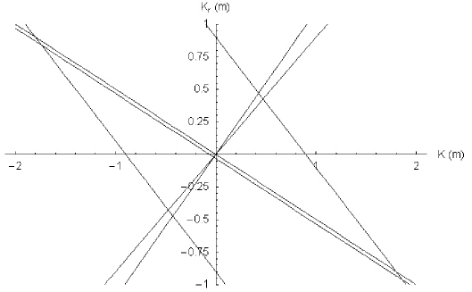
Figure 1: Allowed values for $K$ and $K_{r}$ paper .

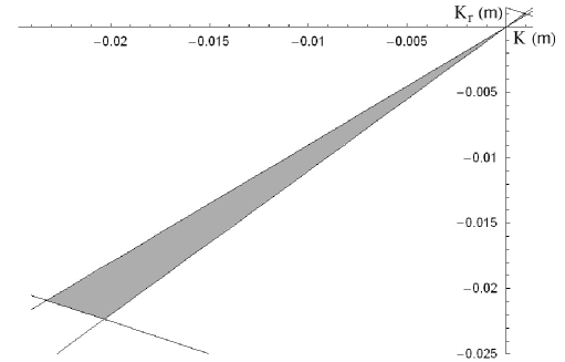
Figure 2: Detail of Fig. $1$, showing only the allowed region paper .

In the limit $M\rightarrow 0$, Eqs. (3) yield $\bar{g}_{tt}=-e^{2K/\xi}$ and $\bar{g}_{rr}=-e^{2K_{r}/\xi}$. An analogy with Rosen’s bimetric theory allows for the PPN parameter $\alpha_{2}$ to be obtained, by interpreting this change of the metric component as due to a background metric $\eta_{\mu\nu}$ Rosen . Notice, however, that the vector field no longer rolls to a radial vev in the absence of a central mass, since this spatial symmetry is inherited from its presence, so this result should be taken with caution; this said, one obtains Will $\alpha_{2}=(c/c_{G})-1=e^{2(K_{r}-K)/\xi}-1\simeq 2(K_{r}-K)/\xi=(A+B)\alpha/\xi$, which has a radial dependency. Assuming $\alpha\simeq 1$ and considering the spin precession constraint arising from solar to ecliptic alignment measurements Will2 , one has $|\alpha_{2}|=|A+B|/r<4\times 10^{-7}$, implying that $|A+B|<4\times 10^{-7}r_{\odot}=2.78\times 10^{2}~{}m$, where $r_{\odot}=6.96\times 10^{8}~{}m$ is the radius of the Sun.

Further pursuing this analogy, we remark that, since there is no explicit Lorentz breaking, the speed of light remains equal to $c$. However, the speed of gravitational waves $c_{G}$ is shifted by an amount

$$\sqrt{c_{G}\over c}=e^{2(K-K_{r})/\xi}\simeq\left[1-{A+B\over\xi}\right]~{}~{},$$ (19)

and hence it acquires a radial dependence. As stated before, this result is highly simplistic and should be taken with caution, since it lacks a complete treatment of gravitational radiation induced by LSB, taking into account variations of the bumblebee field $B_{\mu}$ around its vev $b_{\mu}$.

Finally, notice that, since the radial LSB effects are exact, while the radial/temporal results are not, a direct comparison of these scenarios by taking the $A\rightarrow 0$ limit is not possible.

4 Axial/temporal LSB

The anisotropic LSB case is dealt with in this section. As before, we assume that the bumblebee field is stabilized at its vacuum expectation value, which possesses both a temporal and a spatial component; the latter is taken to lie on the x-axis, that is, $b_{\mu}=\kappa^{-1}(a,b,0,0)$. Since the radial symmetry of the Scharzschild is clearly broken, one cannot resort to a Birkhoff canonical Ansatz. Instead, the perturbations $h_{\mu\nu}$ to the flat Minkowsky metric must be obtained. To first order in $h_{\mu\nu}$, one has

$$R_{00}=-{1\over 2}\nabla^{2}h_{00}~{}~{},~{}~{}R_{0i}=-{1\over 2}\left(\nabla^{2}h_{0i}-h_{k0,ik}\right)~{}~{},$$ (20)

$$R_{ij}=-{1\over 2}\left(\nabla^{2}h_{ij}-h_{00,ij}+h_{kk,ij}-h_{ki,kj}-h_{kj,ki}\right)~{}~{},$$

where time derivatives were neglected, since one assumes that $v\ll c$.

In order to solve the Einstein equations, one first writes the stress-energy tensor for the bumblebee field,

$$T_{B{\mu\nu}}=\left[{1\over 2}b^{\alpha}b^{\beta}R_{\alpha\beta}g_{\mu\nu}-b_{\mu}b^{\alpha}R_{\alpha\nu}-b_{\nu}b^{\alpha}R_{\alpha\mu}\right]~{}~{},$$ (21)

which has a vanishing trace. From the trace of the Einstein equations, one gets

$$R_{\mu\nu}=\kappa\left[T_{\mu\nu}+{1\over 2}g_{\mu\nu}T+T_{B{\mu\nu}}\right]~{}~{}.$$ (22)

To get the $h_{00}$ component to first order in the potential $U$, one writes

$$R_{00}=-{1\over 2}\left(a^{2}R_{00}+b^{2}R_{11}+2abR_{10}\right)-2a\left(aR_{00}+bR_{10}\right)~{}~{},$$ (23)

which, after a little algebra paper , yields the differential equation

$$\left({2+5a^{2}-b^{2}\over 2+5a^{2}}\right)h_{00,11}+h_{00,22}+h_{00,33}=0~{}~{}.$$ (24)

This admits the solution

$$h_{00}(x,y,z)={2M\over\sqrt{c_{0}^{2}x^{2}+y^{2}+z^{2}}}~{}~{},$$ (25)

where $c_{0}^{2}=(2+5a^{2})/(2+5a^{2}-b^{2})$.

Similarly, the $h_{ii}$ components ($i\neq 1$) obey

$$\left(2-b^{2}\right)h_{ii,11}+4h_{ii,ii}+2h_{ii,jj}=\left(a^{2}-b^{2}\right)h_{00,11}+\left(2+a^{2}\right)h_{00,ii}+a^{2}h_{00,jj}~{}~{}.$$ (26)

Taking the Ansatz $h_{ii}(x,y,z)=h_{00}(\alpha_{1}x,\alpha_{2}y,\alpha_{3}z)$ and, after some calculation (see Appendix I of Ref. paper ), one can obtain for the coefficients $\alpha_{i}$:

$$\alpha_{1}^{2}=1-{(2-a^{2})b^{2}\over(2+5a^{2})(2-b^{2})}~{}~{},~{}~{}\alpha_{i}=\alpha_{j}=1~{}~{}.$$ (27)

Hence,

$$h_{ii}(x,y,z)=h_{00}(\alpha_{1}x,y,z)\equiv{2M\over\sqrt{c_{2}^{2}x^{2}+y^{2}+z^{2}}}~{}~{},$$ (28)

with the definition

$$c_{2}^{2}=\alpha_{1}^{2}c_{0}^{2}={2(2+5a^{2}-2b^{2})-4a^{2}b^{2}\over(2+5a^{2}-b^{2})(2-b^{2})}~{}~{}.$$ (29)

The $h_{11}$ component is now computed; a similar calculation leads to the differential equation paper

$$h_{11,22}+h_{11,33}=2M\left[\left({a^{2}(c_{0}^{2}-1)\over 2+3b^{2}}+c_{0}^{2}\right){2c_{0}^{2}x^{2}-y^{2}-z^{2}\over(c_{0}^{2}x^{2}+y^{2}+z^{2})^{5/2}}-2c_{2}^{2}{2c_{2}^{2}x^{2}-y^{2}-z^{2}\over(c_{2}^{2}x^{2}+y^{2}+z^{2})^{5/2}}\right]~{}~{},$$ (30)

indicating that the solution is a linear combination of $h_{00}$ and $h_{22}$. Indeed,

$$h_{11}(x,y,z)=-\left({a^{2}(c_{0}^{2}-1)\over 2+3b^{2}}+c_{0}^{2}\right)h_{00}(x,y,z)+2c_{2}^{2}h_{22}(x,y,z)~{}~{}.$$ (31)

Proceeding to the off-diagonal component $h_{10}$, one obtains the differential equation

$$h_{01,22}+h_{01,33}=-{ab\over 1+a^{2}+b^{2}}\left[h_{00,22}+h_{00,33}+h_{11,22}+h_{11,33}-2h_{22,11}\right]~{}~{}.$$ (32)

Writing $h_{01}=-ab/(1+a^{2}+b^{2})(h_{00}+h_{11}+\delta h_{01})$ leads to

$$\delta h_{01,22}+\delta h_{01,33}=2h_{22,11}={4Mc_{2}^{2}(2c_{2}^{2}x^{2}-y^{2}-z^{2})\over(c_{2}^{2}x^{2}+y^{2}+z^{2})^{5/2}}~{}~{},$$ (33)

and hence $\delta h_{01}(x,y,z)=-2c_{2}^{2}h_{22}(x,y,z)$. Therefore,

$$h_{01}={ab\over 1+a^{2}+b^{2}}\left[{a^{2}(c_{0}^{2}-1)\over 2+3b^{2}}+c_{0}^{2}\right]h_{00}~{}~{}.$$ (34)

Finally, the $h_{00}$ component is computed to second order (see Appendix II of Ref. paper ); it can be shown that only a correction to the first order term $h_{00}^{(1)}$ appears:

$$h_{00}={2c_{0}^{2}[6+9b^{2}+(15+22b^{2})a^{2}]+a^{2}b^{2}\over c_{0}^{2}(6+15a^{2}+b^{2})(2+3b^{2})}h_{00}^{(1)}\simeq\left(1-{b^{2}\over 6}\right)h_{00}^{(1)}~{}~{}.$$ (35)

The PPN formalism cannot be straightforwardly used to ascertain its effects, since it relies on a transformation to a quasi-cartesian frame of reference on which, by definition, all diagonal metric components $g_{ii}$ are equal. However, some PPN-like parameters may be extracted from the results, by noticing that

$${1\over\sqrt{(1+2k)x^{2}+y^{2}+z^{2}}}\simeq{1\over r}\left(1-kcos^{2}\theta\right)~{}~{}.$$ (36)

For $h_{00}$, one gets

$$h_{00}=\left(1-{b^{2}\over 6}\right)2M{1-(c_{0}^{2}-1)cos^{2}\theta\over r}~{}~{}.$$ (37)

Since no $r^{-2}$ correction appears, the PPN parameter $\beta$ vanishes in this approach. However, as $h_{11}\neq h_{22}=h_{33}$, the same reasoning allows two parameters analogous to the $\gamma$ PPN parameter to be obtained: after neglecting the normalization with respect to $h_{00}$, one gets

$$\gamma_{1} = 1+cos^{2}\theta\times\left[-\left[{a^{2}(c_{0}^{2}-1)\over 2+3b^{2}}+c_{0}^{2}\right](1-c_{0}^{2})+2c_{2}^{2}(1-c_{2}^{2})\right]\simeq 1+{b^{2}\over 2}cos^{2}\theta~{}~{},$$

$$\gamma_{2} = 1+(1-c_{2}^{2})cos^{2}\theta\simeq 1-\left({ab\over 2}\right)^{2}cos^{2}\theta~{}~{}.$$ (38)

As expected, the x-axis LSB produces a stronger effect on the $h_{11}$ component. No clear connection can be derived to link $\gamma$ with $\gamma_{1}$ and $\gamma_{2}$, due to the aforementioned anisotropy. However, one can take $\gamma$ to be of the same order of magnitude as the average of $\gamma_{1}$ and $\gamma_{2}$, integrated over one orbit:

$$\gamma-1\simeq{1\over 2}(\gamma_{1}+\gamma_{2})-1\simeq{b^{2}\over 4}\langle cos^{2}\theta\rangle\simeq{b^{2}\over 8}(1-e^{2})~{}~{},$$ (39)

where $e$ is the orbit eccentricity. For low values of $e$, one gets $\gamma\simeq b^{2}/8$; The constraint $\gamma=1+(2.1\pm 2.3)\times 10^{-5}$ then enables $|b|\leq 1.9\times 10^{-2}$.

A discussion concerning the anisotropy of inertia and its effect in the width of resonance lines has been presented as a test between Mach’s principle and the Equivalence Principle Weinberg ; Kostelecky6 , relying on the hypothetical effect on the proton mass of the proximity to the galactic core. In the present scenario, we note that a radial LSB with the galactic core acting as source would amount to an axial LSB in a small region such as the Solar System. The bound $\Delta m_{P}/m_{P}\leq 3\times 10^{-22}$, $m_{P}$ being the proton mass Lamoreaux , can then be used to obtain

$${\Delta m_{P}\over m_{P}}=\left(1-{b^{2}\over 6}\right)(c_{0}^{2}-1)\simeq{b^{2}\over 2}\leq 3\times 10^{-22}~{}~{},$$ (40)

resulting in the limit $|b|\leq 2.4\times 10^{-11}$, a much more stringent bound than the obtained above.

5 Conclusions

In this contribution, the solutions of a gravity model coupled to a vector field where Lorentz symmetry is spontaneously broken are studied, and three different relevant scenarios were highlighted: a purely radial, temporal/radial and temporal/axial LSB.

In the first case, a new black hole solution is found, exhibiting a removable singularity at a horizon of radius $r_{s}=(2Mr_{0}^{-L})^{1/1-L}$, slightly perturbed with respect to the usual Scharzschild radius $r_{s0}=2M$. This has an associated Hawking temperature of $T=(2Mr_{0}^{-L})^{-L}T_{0}$, where $T_{0}=\hbar/8\pi\kappa_{B}M$ is the usual Hawking temperature, and protects an intrinsic singularity at $r=0$. Bounds on deviations from Kepler’s law yield $L\leq 2\times 10^{-9}$.

The temporal/radial scenario produces a slightly perturbed metric that leads to the PPN parameters $\beta\approx 1-(K+K_{r})/M$ and $\gamma\approx 1-(K+2K_{r})/M$, directly proportional to the strength of the derived effect (given by $K$ and $K_{r}\sim K$). Since $K$ and $K_{r}$ are integration constants, no constraints on the physical parameters may be derived from the observed limits on the PPN parameters. Also, an analogy with Rosen’s bimetric theory, yields the PPN parameter $\gamma\simeq(A+B)\xi$, $\xi$ being the distance to the central body and $A$ and $B$ parameters ruling the temporal and radial components of the vector field vev.

In the temporal/axial scenario, a breakdown of isotropy is obtained, disallowing a standard PPN analysis. However, the direction-dependent “PPN” parameters $\gamma_{1}\simeq b^{2}cos^{2}\theta/2$ and $\gamma_{2}\simeq a^{2}b^{2}cos^{2}\theta/4$ may be derived, where $a$ and $b$ are respectively the temporal and $x$-component of the bumblebee vector vev; naturally, $\gamma_{1}\ll\gamma_{2}$. A crude estimative of the PPN parameter $\gamma$ yields $\gamma\approx b^{2}(1-e^{2})/4$, where $e$ is the orbit’s eccentricity. Furthermore, a comparison with experiments concerning the anisotropy of inertia produces the bounds $|b|\leq 2.4\times 10^{-11}$.

References

(1) “CPT and Lorentz Symmetry II”, Ed., V. A. Kostelecký (World
Scientific, Singapore, 2002).
(2) O. Bertolami, Nucl. Phys. Proc. Suppl. 88, 49
(2000); O. Bertolami in “Decoherence and Entropy in Complex
Systems” (Springler-Verlag, Berlin, 2004).
(3) V. A. Kostelecký and S. Samuel, Phys. Rev.D 39, 683
(1989); Phys. Rev. Lett.66, 1811 (1991).
(4) V. A. Kostelecký and R. Potting, Phys. Rev.D 51, 3923 (1995).
(5) V. A. Kostelecký, Phys. Rev.D 69, 105009 (2004).
(6) R. Bluhm and V. A. Kostelecký, hep-th/0412320.
(7) S. M. Carroll, J. A. Harvey, V. A. Kostelecký, C. D.
Lane and T. Okamoto, Phys. Rev. Lett.87, 141601 (2001).
(8) O. Bertolami and L. Guisado, Phys. Rev.D 67, 025001 (2003); JHEP0312,
O13 (2003); O. Bertolami, Mod. Phys. Lett.A 20, 1359 (2005).
(9) V.A. Kostelecký, R. Lehnert and M. J. Perry, Phys. Rev.D 68, 123511
(2003) ; O. Bertolami, R. Lehnert, R. Potting and A. Ribeiro, Phys. Rev.D 69, 083513 (2004).
(10) H. Sato and T. Tati, Progr. Theor. Phys.47, 1788 (1972); S.
Coleman and S.L. Glashow, Phys. Lett.B 405, 249 (1997); Phys. Rev.D
59, 116008 (1999); O. Bertolami and C.S. Carvalho, Phys. Rev.D
61, 103002 (2000); O. Bertolami, Gen. Relativity and Gravitation34 707 (2002); R.
Lehnert, hep-ph/0312093.
(11) O. Bertolami and J. Páramos, Phys. Rev.D 72, 044001 (2005).
(12) R. Grard, M. Novara and G. Scoon, ESA Bull.103, 11
(2000); L. Iorio, I. Ciufolini and E. C. Pavlis, Class. Quantum Gravity19,
4301 (2002).
(13) S. G. Turyshev et al., gr-qc/0505064.
(14) O. Bertolami, J. Páramos and S. G. Turyshev,
gr-qc/0601016.
(15) M. C. Bento and O. Bertolami, Phys. Lett.B 228, 348
(1999).
(16) E.
Fischbach and C.L. Talmadge, “The search for non-Newtonian
gravity” (Springer, New York 1999).
(17) C. M. Will, Living Rev. Rel. 4, 4 (2001).
(18) B. Bertotti, L. Iess and P. Tortora, Nature 425, 374 (2003).
(19) N. Rosen, J. Gen. Rel. and Grav.4, 435 (1973).
(20) C.M. Will, “Theory and Experiment in Gravitational Physics”,
C.M. Will (Cambridge U. P., 1993).
(21) S. Weinberg, “Gravitation and Cosmology: Principles and Applications of the
General Theory of Relativity” (John Wiley and Sons, New Jersey,
1972).
(22) V. A. Kostelecký and C. D. Lane, J. Math. Phys. 40
6245 (1999).
(23) S. K. Lamoreaux, J. P. Jacobs, B. R. Heckel, F. J. Raab, and E. N. Fortson,
Phys. Rev. Lett.58, 746 (1987).