Phasing of gravitational waves from inspiralling eccentric binaries at the third-and-a-half post-Newtonian order

Abstract

We obtain an efficient description for the dynamics of nonspinning compact binaries moving in inspiralling eccentric orbits to implement the phasing of gravitational waves from such binaries at the 3.5 post-Newtonian (PN) order. Our computation heavily depends on the phasing formalism, presented in [T. Damour, A. Gopakumar, and B. R. Iyer, Phys. Rev. D 70, 064028 (2004)], and the 3PN accurate generalized quasi-Keplerian parametric solution to the conservative dynamics of nonspinning compact binaries moving in eccentric orbits, available in [R.-M. Memmesheimer, A. Gopakumar, and G. Schäfer, Phys. Rev. D 70, 104011 (2004)]. The gravitational-wave (GW) polarizations $h_{+}$ and $h_{\times}$ with 3.5PN accurate phasing should be useful for the earth-based GW interferometers, current and advanced, if they plan to search for gravitational waves from inspiralling eccentric binaries. Our results will be required to do astrophysics with the proposed space-based GW interferometers like LISA, BBO, and DECIGO.

I Introduction

Inspiralling compact binaries of arbitrary mass ratio moving in quasi-circular orbits are the most plausible sources of gravitational radiation for the first generation ground-based interferometric detectors GWIFs . The availability of highly accurate general relativistic theoretical waveforms required to extract the weak GW signals from the noise-dominated interferometric data is the main reason for the above understanding. The dynamics of long lived and isolated compact binaries can be modelled accurately in the PN approximation to general relativity as point particles moving in quasi-circular orbits. The PN approximation allows one to express the equations of motion of a compact binary as corrections to the Newtonian equations of motion in powers of $(v/c)^{2}\sim GM/(c^{2}R)$, where $v$, $M$, and $R$ are the characteristic orbital velocity, the total mass, and the typical orbital separation of the binary, respectively. Recently, the orbital evolution of nonspinning compact binaries in quasi-circular orbits, under the action of general relativity, was computed up to the 3.5PN order in Ref. ref1NEW . The amplitude corrections to the GW polarizations $h_{+}$ and $h_{\times}$ are also available to the 2.5PN order ABIQ04 .

However, a recent surge in astrophysically motivated investigations indicates that compact binaries of arbitrary mass ratio moving in inspiralling eccentric orbits are also plausible sources of gravitational radiation even for the ground-based GW interferometers. One of the earliest scenarios involves Kozai oscillations, associated with hierarchical triplets that may be present in globular clusters K62 ; MH02 ; Rasio2000 ; W03 . Last year, it was pointed out that during the late stages of black hole–neutron star (BH–NS) inspiral the binary can become eccentric DLK05 . This is because in general the neutron star is not disrupted at the first phase of mass transfer and what remains of the neutron star is left on a wider eccentric orbit from where it again inspirals back to the black hole. This scenario was very recently invoked to explain the light curve of the short gamma-ray burst GRB $050911$ Page05 . Another scenario, reported in Nature, suggests that at least partly short GRBs are produced by the merger of NS–NS binaries, formed in globular clusters by exchange interactions involving compact objects GZM_nature_2006 . A distinct feature of such binaries is that they have high eccentricities at short orbital separation [see Fig. 2 in Ref. GZM_nature_2006 ]. Compact binaries that merge with some residual eccentricities may be present in galaxies too. Chaurasia and Bailes demonstrated that a natural consequence of an asymmetric kick imparted to neutron stars at birth is that the majority of NS–NS binaries should possess highly eccentric orbits CB05 . Further, the observed deficit of highly eccentric short-period binary pulsars was attributed to selection effects in pulsar surveys. The authors also pointed out that their conclusions are applicable to BH–NS and BH–BH binaries. Yet another scenario that can create inspiralling eccentric binaries with short periods involves compact star clusters. It was noted that the interplay between GW-induced dissipation and stellar scattering in the presence of an intermediate-mass black hole can create short-period highly eccentric binaries HA05_ApJ . Finally, a very recent attempt to model realistically compact clusters that are likely to be present in galactic centers indicates that compact binaries usually merge with eccentricities RS_MNRAS . These above mentioned scenarios force us to claim that compact binaries in inspiralling eccentric orbits are plausible sources of gravitatinal waves even for the ground-based GW interferometers.

In order to do astrophysics with the proposed space-based GW interferometers, LISA LISA , BBO BBOproposal , and DECIGO DECIGO , it is required to have highly accurate GW polarizations, $h_{+}$ and $h_{\times}$, from compact binaries of arbitrary mass ratio moving in inspiralling eccentric orbits. Recall, the earlier discussions also indicate that stellar-mass compact binaries in eccentric orbits are excellent sources for LISA. Furthermore, it is expected that LISA will “hear” gravitational waves from intermediate-mass black holes moving in highly eccentric orbits Gultekin05 ; M05 ; GFR05 . Finally, several papers which appeared recently in the arXiv indicate that supermassive black-hole binaries, formed from galactic mergers, may coalesce with orbital eccentricity SA02 ; RS_SMBHbinary ; BLS02 ; AN05 ; IFM05 . It is interesting to note that these investigations employ different techniques and astrophysical scenarios to reach the above conlusion.

The above mentioned astrophysically inspired investigations motivated us to extend the phasing formalism, developed and implemented with 2.5PN accuracy in Ref. DGI , to the next PN order, namely, the 3.5PN order. The phasing formalism provides a method to construct, almost analytically, templates for compact binaries of arbitrary mass ratio moving in inspiralling eccentric orbits.

We recall that accurate templates for the detection of gravitational waves require phasing, i.e., an accurate mathematical modelling of the continous time evolution of the GW polarizations. In the case of inspiralling eccentric binaries, the above modelling requires the combination of three different time scales present in the dynamics, namely, those associated with the radial motion (orbital period), advance of periastron, and radiation reaction, without treating radiation reaction in an adiabatic mannner. In Ref. DGI , an improved method of variation of constants was presented to combine these three time scales and to obtain the phasing at the 2.5PN order. We note that the techniques adapted in Ref. DGI were influenced by the mathematical formulation, developed by Damour TD82 ; TD83 ; TD_F85 , that gave the (heavily employed) accurate relativistic timing formula for binary pulsars DD86 ; DT92 .

It is possible to extend the phasing to the 3.5PN order, mainly because of the recent determination of the 3PN accurate generalized quasi-Keplerian parametric solution to the conservative dynamics of nonspinning compact binaries of arbitrary mass ratio moving in eccentric orbits MGS . This parametrization, presented in Ref. MGS , allows one to solve analytically the 3PN accurate conservative dynamics of nonspinning compact binaries, computed both in ADM-type coordinates DJS00A and in harmonic coordinates BF01 , indicating the deterministic nature of the underlying dynamics GK05nochaos . Further, we recall that Ref. MGS extends the quasi-Keplerian parametrization developed by Damour and his collaborators DD85 ; DS88 ; SW93 , which is crucial to construct the timing formula relevant for relativistic binary pulsars DD86 ; DT92 . This observation clearly reveals the link, as envisaged by Damour, connecting GW observations of inspiralling compact binaries to the timing of binary pulsars. In Ref. DGI , explicit computations to realize the phasing at the 2.5PN order were done in ADM coordinates as at that time the 2PN accurate generalized quasi-Keplerian parametrization, required by the method of variation of constants, was only available in ADM coordinates. However, in this paper, computations required for the phasing at the 3.5PN order are done in harmonic coordinates. Harmonic coordinates are preferred as computations that lead to ready to use search templates for compact binaries in quasi-circular orbits are usually performed in harmonic gauge ref1NEW .

This paper has the following plan. In Sec. II, we outline the procedure, detailed in Ref. DGI , to perform the phasing. Section III provides explicit formulae required for the 3.5PN accurate phasing, which also include 3.5PN accurate equations for the secular and periodic variations of the orbital elements involved in the phasing. The pictorial representation of the main results and the related discussions are presented in Sec. IV. Finally, in Sec. V, we give a brief summary and point out possible extensions. Appendices A and B deal with computational details and some supplementary results.

II Brief description of GW phasing for inspiralling eccentric binaries

In this section, we summarize the basic ideas of GW phasing, as detailed in Ref. DGI . We also discuss what is required for this purpose and how the method of variation of constants will be invoked.

II.1 Basic structure of GW phasing

Let us first describe the method, developed in Ref. DGI , to implement the GW phasing for compact binaries in inspiralling eccentric orbits. The theoretical templates required by the GW interferometers consist of the two independent GW polarization states $h_{+}$ and $h_{\times}$. The appropriate expressions for $h_{+}$ and $h_{\times}$, expressed in terms of the binary’s intrinsic dynamical variables and location, are given by

$$h_{+} =\frac{1}{2}(p_{i}p_{j}-q_{i}q_{j})h_{ij}^{\rm TT}\,,$$ (1a)

$$h_{\times} =\frac{1}{2}(p_{i}q_{j}+p_{j}q_{i})h_{ij}^{\rm TT}\,,$$ (1b)

where $h_{ij}^{\rm TT}$ is the transverse-traceless (TT) part of the radiation field. The two orthogonal unit vectors $\bm{p}$ and $\bm{q}$ span the plane of the sky, i.e., the plane transverse to the radial direction linking the source to the observer.

The TT radiation field is given, by the existing GW generation formalisms BDIWW ; BIWW96 ; WW96 ; ref1NEW ; ABIQ04 , as a PN expansion in $(v/c)$. In this paper, for simplicity, we will restrict $h_{ij}^{\rm TT}$ to its leading “quadrupolar” order and denote it by $h_{ij}^{\rm TT}|_{\rm Q}$. However, higher-PN corrections to $h_{ij}^{\rm TT}$ are available in the existing literature WW96 ; GI97 . The explicit expression for $h_{ij}^{\rm TT}|_{\rm Q}$, in terms of the relative separation vector $\bm{r}$ and the relative velocity vector $\bm{v}$, reads

$$h_{km}^{\rm TT}\big{|}_{\rm Q} =\frac{4G\mu}{c^{4}R^{\prime}}\mathcal{P}_{ijkm}(\bm{N})\left(v_{i}v_{j}-\frac{GM}{r}n_{i}n_{j}\right)\,,$$ (2)

where $\mathcal{P}_{ijkm}(\bm{N})$ is the usual TT projection operator projecting normal to $\bm{N}$, where $\bm{N}=\bm{R}^{\prime}/R^{\prime}$ is the line-of-sight unit vector from the binary to the observer, and $R^{\prime}=|\bm{R}^{\prime}|$ is the corresponding radial distance. The reduced mass of the binary $\mu$ is given by $m_{1}m_{2}/M$, where $M\equiv m_{1}+m_{2}$ is the total mass of the binary consisting of individual masses $m_{1}$ and $m_{2}$. The components of the unit relative separation vector $\bm{n}=\bm{r}/r$, where $r=|\bm{r}|$, and the velocity vector $\bm{v}=d\bm{r}/dt$ are denoted by $n_{i}$ and $v_{i}$, respectively.

In order to compute $h_{+}|_{\rm Q}$ and $h_{\times}|_{\rm Q}$, the expressions for the GW polarization states when their amplitudes are restricted to the leading quadrupolar order, one needs to choose a convention for the direction and orientation of the orbital plane with respect to the plane of sky. We follow the convention used in Refs. DGI ; WW96 ; BIWW96 for choosing the orthonormal triad $(\bm{p},\bm{q},\bm{N})$ — $\bm{N}$ from the source to the observer and $\bm{p}$ toward the correspondingly defined ascending node — and use $\bm{r}=r\cos\phi\bm{p}+r\sin\phi(\cos i\bm{q}+\sin i\bm{N})$, where $i$ denotes the inclination angle of the orbital plane with respect to the plane of the sky. This leads to the following lowest-order contributions to the two independent GW polarization states as functions of the relative separation $r$ and the true anomaly $\phi$, i.e., the polar angle of $\bm{r}$, and their time derivatives $\dot{r}$ and $\dot{\phi}$, which read DGI

$$h_{+}(r,\phi,\dot{r},\dot{\phi})\big{|}_{\rm Q} =-\frac{G\mu}{c^{4}R^{\prime}}\bigg{\{}(1+C^{2})\bigg{[}2\dot{r}r\dot{\phi}\sin 2\phi$$

$$\quad+\bigg{(}\frac{GM}{r}+r^{2}\dot{\phi}^{2}-\dot{r}^{2}\bigg{)}\cos 2\phi\bigg{]}$$

$$\quad+S^{2}\bigg{(}\frac{GM}{r}-r^{2}\dot{\phi}^{2}-\dot{r}^{2}\bigg{)}\bigg{\}}\,,$$ (3a)

$$h_{\times}(r,\phi,\dot{r},\dot{\phi})\big{|}_{\rm Q} =-\frac{2G\mu C}{c^{4}R^{\prime}}\bigg{[}\bigg{(}\frac{GM}{r}+r^{2}\dot{\phi}^{2}-\dot{r}^{2}\bigg{)}\sin 2\phi$$

$$\quad-2\dot{r}r\dot{\phi}\cos 2\phi\bigg{]}\,,$$ (3b)

where $C$ and $S$ are shorthand notations for $\cos i$ and $\sin i$, respectively. The orbital phase is denoted by $\phi$, $\dot{\phi}=d\phi/dt$, and $\dot{r}=dr/dt=\bm{n}\cdot\bm{v}$.

In order to achieve the GW phasing for compact binaries of arbitrary mass ratio moving in inspiralling eccentric binaries, we need to provide explicit expressions describing the temporal evolution of $r(t)$, $\phi(t)$, $\dot{r}(t)$, and $\dot{\phi}(t)$, the only dynamical variables appearing in Eqs. (3). Following Ref. DGI , we refer to, as phasing, an explicit way to define the latter time dependences. This is the crucial input to derive ready to use waveforms $h_{+}(t)$ and $h_{\times}(t)$. Adapting the formalism presented in Ref. DGI , we will provide the above desired time evolution to the 3.5PN order in an almost parametric manner.

However, there are a few points that we want to clarify before we describe the above procedure. First, as explained in Ref. DGI , the possibility of obtaining explicit expressions for the GW polarizations $h_{+}|_{\rm Q}$ and $h_{\times}|_{\rm Q}$ in terms of the relative dynamics, specified by $r(t)$, $\phi(t)$, $\dot{r}(t)$, and $\dot{\phi}(t)$, relies on the possibility of going to a suitable defined center-of-mass (COM) frame. Though such a frame exists only to the 3PN order BI02 , we will not worry about the associated “recoil” of the center of mass at the 3.5PN order. This is because, as demonstrated in Ref. DGI , the influence of the recoil on waveforms appears at the 4PN order and we may safely neglect it for the present computation.

A second point, again detailed in Ref. DGI , is that the GW polarizations $h_{+}|_{\rm Q}$ and $h_{\times}|_{\rm Q}$ only depend on the temporal evolution of $r(t)$, $\phi(t)$, $\dot{r}(t)$, and $\dot{\phi}(t)$, as we are dealing with nonspinning compact objects. In the presence of spin interactions, the orbital plane is no longer fixed in space and one needs to introduce further variables DT92 ; KG05_so_para ; KG06_k_obs ; DS88 . However, expressions for $h_{+}|_{\rm Q}$ and $h_{\times}|_{\rm Q}$, valid for spinning compact binaries are recently obtained in Ref. KG05_so_para and the phasing for such binaries will be reported elsewhere.

Finally, we want to discuss the choice of the underlying coordinate system. Though the explicit functional forms of $h_{+}(r,\phi,\dot{r},\dot{\phi})|_{\rm Q}$ and $h_{\times}(r,\phi,\dot{r},\dot{\phi})|_{\rm Q}$, as well as the phasing relations $r(t)$, $\phi(t)$, $\dot{r}(t)$, and $\dot{\phi}(t)$ depend on the used coordinate system, the final results $h_{+}(t)$ and $h_{\times}(t)$ do not. Note that $h_{ij}^{\rm TT}$ and therefore $h_{+}(t)$ and $h_{\times}(t)$ are coordinate independent asymptotic quantities. In this paper, we consistently work in harmonic coordinates because (i) they will allow us to write down explicit analytical expressions for the orbital phasing $r(t)$, $\phi(t)$, $\dot{r}(t)$, and $\dot{\phi}(t)$, based on Ref. MGS , and (ii) the harmonic coordinate systems are used in the standard GW generation formalisms to derive the amplitude expressions, giving higher-PN corrections to $h_{ij}^{\rm TT}$.

In the next subsection, we will explain a version of the general Lagrange method of variation of arbitrary constants, which was employed to compute, within general relativity, the orbital evolution of the Hulse-Taylor binary pulsar TD83 ; TD_F85 , and applied for the 2.5PN accurate phasing in Ref. DGI .

II.2 Improved method of variation of constants and its implementation at the 3.5PN order

The method, presented in Ref. DGI , begins by splitting the relative acceleration $\bm{\mathcal{A}}$ of the compact binary into two parts, an integrable leading part $\bm{\mathcal{A}}_{0}$ and a perturbative part $\bm{\mathcal{A}}^{\prime}$, as $\bm{\mathcal{A}}=\bm{\mathcal{A}}_{0}+\bm{\mathcal{A}}^{\prime}$. The method first constructs the solution to the “unperturbed” system, defined by

$$\dot{\bm{r}} =\bm{v}\,,$$ (4a)

$$\dot{\bm{v}} =\bm{\mathcal{A}}_{0}(\bm{r},\bm{v}).$$ (4b)

The solution to the exact system

$$\dot{\bm{r}} =\bm{v}\,,$$ (5a)

$$\dot{\bm{v}} =\bm{\mathcal{A}}(\bm{r},\bm{v})\,,$$ (5b)

is then obtained by varying the constants in the generic solution of the unperturbed system, given by Eqs. (4).

In this paper, we work to the 3.5PN order and therefore $\bm{\mathcal{A}}_{0}$ will be the acceleration at the 3PN order and $\bm{\mathcal{A}}^{\prime}$ contains the reactive 2.5PN and 3.5PN contributions. The method assumes — as is true for $\bm{\mathcal{A}}_{\rm 3PN}^{\rm conservative}$ — that the unperturbed system admits sufficiently many integrals of motion to be integrable. At the 3PN order with $\bm{\mathcal{A}}_{0}=\bm{\mathcal{A}}_{\rm 3PN}$, we have four first integrals: the 3PN accurate energy and the 3PN accurate angular-momentum vector of the binary. We denote these quantities, written in the 3PN accurate COM frame by $c_{1}$ and $c_{2}^{i}$:

$$c_{1} ={E}(\bm{r},\bm{v})\big{|}_{\rm 3PN\leavevmode\nobreak\ COM}\,,$$ (6a)

$$c_{2}^{i} ={L}_{i}(\bm{r},\bm{v})\big{|}_{\rm 3PN\leavevmode\nobreak\ COM}\,.$$ (6b)

At the 3PN order, the functional form of the solution to the unperturbed equations of motion in the COM frame, following Refs. TD83 ; MGS , may be expressed as

$$r =S(l;c_{1},c_{2})\,,$$ (7a)

$$\dot{r} =n\frac{\partial S}{\partial l}(l;c_{1},c_{2})\,,$$ (7b)

$$\phi =\lambda+W(l;c_{1},c_{2})\,,$$ (7c)

$$\dot{\phi} =(1+k)n+n\frac{\partial W}{\partial l}(l;c_{1},c_{2})\,,$$ (7d)

where $\lambda$ and $l$ are two basic angles, which are $2\pi$ periodic, and $c_{2}=|c_{2}^{i}|$. The functions $S(l)$ and $W(l)$ and hence their derivatives $\frac{\partial S}{\partial l}(l)$ and $\frac{\partial W}{\partial l}(l)$ are also periodic in $l$. In the above equations, $n$ denotes the unperturbed “mean motion”, given by $n=2\pi/P$, $P$ being the radial (periastron to periastron) period, while $k=\Delta\Phi/(2\pi)$, where $\Delta\Phi$ represents the advance of periastron in the time interval $P$. The explicit 3PN accurate expressions for $P$ and $k$ in terms of $c_{1}$ and $c_{2}$ are obtainable from Refs. MGS ; DJS00B . The angles $l$ and $\lambda$ satisfy, still for the unperturbed system, $\dot{l}=n$ and $\dot{\lambda}=(1+k)n$, which integrate to

$$l =n(t-t_{0})+c_{l}\,,$$ (8a)

$$\lambda =(1+k)n(t-t_{0})+c_{\lambda}\,,$$ (8b)

where $t_{0}$ is some initial instant and the constants $c_{l}$ and $c_{\lambda}$ are the corresponding values for $l$ and $\lambda$. Note that the unperturbed solution depends on four integration constants: $c_{1}$, $c_{2}$, $c_{l}$, and $c_{\lambda}$.

Before we explain the prescription to obtain the phasing at the 3.5PN order, let us first present our description of the 3PN accurate conservative dynamics. The 3PN accurate parametric solution to the dynamics of compact binaries of arbitrary mass ratio moving in eccentric orbits, derived in Ref. MGS , allows us to describe the orbital motion in the 3PN accurate COM frame. The vectorial structure of $c_{2}^{i}$ [see Eq. (6b)], indicates that the unperturbed 3PN accurate motion takes place in a plane, the so-called orbital plane. The problem is restricted to a plane even in the presence of radiation reaction. Therefore, we introduce polar coordinates in the orbital plane, $r$ and $\phi$, such that the relative separation vector $\bm{r}$ takes the following form $\bm{r}=r\cos\phi\bm{i}+r\sin\phi\bm{j}$, where we may choose $\bm{i}=\bm{p}$ and $\bm{j}=\cos i\bm{q}+\sin i\bm{N}$ as the definition for the basic vectors. The dynamical variables $r$ and $\phi$, available in Ref. MGS , are parametrically given by

$$r =a_{r}\left(1-e_{r}\cos u\right)\,,$$ (9a)

$$\phi-\phi_{0} =(1+k)v+\bigg{(}\frac{f_{4\phi}}{c^{4}}+\frac{f_{6\phi}}{c^{6}}\bigg{)}\sin 2v$$

$$\quad+\bigg{(}\frac{g_{4\phi}}{c^{4}}+\frac{g_{6\phi}}{c^{6}}\bigg{)}\sin 3v+\frac{i_{6\phi}}{c^{6}}\sin 4v$$

$$\quad+\frac{h_{6\phi}}{c^{6}}\sin 5v\,,$$ (9b)

$$\text{where}\quad v =2\arctan\left[\left(\frac{1+e_{\phi}}{1-e_{\phi}}\right)^{1/2}\tan\frac{u}{2}\right]\,.$$ (9c)

In the above equations, $a_{r}$, $e_{r}$, and $e_{\phi}$ are some 3PN accurate semimajor axis, radial eccentricity, and angular eccentricity, respectively, while $f_{4\phi}$, $f_{6\phi}$, $g_{4\phi}$, $g_{6\phi}$, $i_{6\phi}$, and $h_{6\phi}$ are some PN accurate orbital functions. The following 3PN accurate Kepler equation connects the eccentric anomaly $u$ (and hence the true anomaly $v$) to the coordinate time $t$ and reads

$$l\equiv n\left(t-t_{0}\right) =u-e_{t}\sin u+\bigg{(}\frac{g_{4t}}{c^{4}}+\frac{g_{6t}}{c^{6}}\bigg{)}(v-u)$$

$$\quad+\bigg{(}\frac{f_{4t}}{c^{4}}+\frac{f_{6t}}{c^{6}}\bigg{)}\sin v+\frac{i_{6t}}{c^{6}}\sin 2v$$

$$\quad+\frac{h_{6t}}{c^{6}}\sin 3v\,.$$ (10)

Here $e_{t}$ denotes some time eccentricity and $g_{4t}$, $g_{6t}$, $f_{4t}$, $f_{6t}$, $i_{6t}$, and $h_{6t}$ are some PN accurate orbital functions. All these PN accurate orbital elements and functions, expressible in terms of $c_{1}$, $c_{2}$, and $\eta\equiv\mu/M$, are available in Ref. MGS .

With the help of the above 3PN accurate parametric solution, we write down explicit expressions for the functions $S(l)$ and $W(l)$:

$$S(l;c_{1},c_{2}) =a_{r}(1-e_{r}\cos u)\,,$$ (11a)

$$W(l;c_{1},c_{2}) =(1+k)(v-l)+\bigg{(}\frac{f_{4\phi}}{c^{4}}+\frac{f_{6\phi}}{c^{6}}\bigg{)}\sin 2v$$

$$\quad+\bigg{(}\frac{g_{4\phi}}{c^{4}}+\frac{g_{6\phi}}{c^{6}}\bigg{)}\sin 3v+\frac{i_{6\phi}}{c^{6}}\sin 4v$$

$$\quad+\frac{h_{6\phi}}{c^{6}}\sin 5v\,.$$ (11b)

We emphasize that for the phasing the anomalies $v$ and $u$ in Eqs. (11) have to be expressed as functions of $l$, $c_{1}$, and $c_{2}$. This can be achieved in the following way, written symbolically as $v=\mathcal{V}(l;c_{1},c_{2})=V[\mathcal{U}(l;c_{1},c_{2})]$ and $u=\mathcal{U}(l;c_{1},c_{2})$. First, recall that the function $v\equiv V(u)$ is defined by Eq. (9c), and second, the function $u=\mathcal{U}(l)$ is defined by inverting the Kepler equation $l=l(u)$, given by Eq. (II.2). Finally, the function $v=\mathcal{V}(l)$ is obtained by inserting $u=\mathcal{U}(l)$ in $v=V(u)$, i.e., $v=\mathcal{V}(l)\equiv V[\mathcal{U}(l)]$.

In our computations, we use the following exact relation for $v-u$, which is also periodic in $u$:

$$v-u =2\tan^{-1}\left(\frac{\beta_{\phi}\sin u}{1-\beta_{\phi}\cos u}\right)\,,$$ (12)

where $\beta_{\phi}=(1-\sqrt{1-e_{\phi}^{2}})/e_{\phi}$ [for the derivation of Eq. (12), see Appendix A].

In line with the method of variation of constants, we write down the following general solution to the reactive 3.5PN accurate dynamics, Eqs. (5), as

$$r =S(l;c_{1},c_{2})\,,$$ (13a)

$$\dot{r} =n\frac{\partial S}{\partial l}(l;c_{1},c_{2})\,,$$ (13b)

$$\phi =\lambda+W(l;c_{1},c_{2})\,,$$ (13c)

$$\dot{\phi} =(1+k)n+n\frac{\partial W}{\partial l}(l;c_{1},c_{2})\,.$$ (13d)

However, the constants $c_{1}$ and $c_{2}$, appearing in Eqs. (7), are now functions of time in Eqs. (13): $c_{1}=c_{1}(t)$ and $c_{2}=c_{2}(t)$. The temporal variation of the basic angles $l$ and $\lambda$, entering Eqs. (13), is now given by

$$l \equiv\int_{t_{0}}^{t}ndt+c_{l}(t)\,,$$ (14a)

$$\lambda \equiv\int_{t_{0}}^{t}(1+k)ndt+c_{\lambda}(t)\,,$$ (14b)

involving two new temporally evolving quantities $c_{l}(t)$ and $c_{\lambda}(t)$. In the method of variation of constants, we search for solutions of the exact system, Eqs. (5), in the form given by Eqs. (13) and (14) with four “varying constants”: $c_{1}(t)$, $c_{2}(t)$, $c_{l}(t)$, and $c_{\lambda}(t)$. These four new variables replace the original four dynamical variables $r(t)$, $\dot{r}(t)$, $\phi(t)$, and $\dot{\phi}(t)$, and satisfy, like the original phase-space variables, first-order evolution equations TD83 ; TD_F85 . These first-order evolution equations for $c_{1}(t)$, $c_{2}(t)$, $c_{l}(t)$, and $c_{\lambda}(t)$ are available in Refs. DGI ; TD_F85 and read in our notation

$$\frac{dc_{1}}{dt} =\frac{\partial c_{1}(\bm{r},\bm{v})}{\partial v^{i}}{\mathcal{A}^{\prime}}^{i}\,,$$ (15a)

$$\frac{dc_{2}}{dt} =\frac{\partial c_{2}(\bm{r},\bm{v})}{\partial v^{j}}{\mathcal{A}^{\prime}}^{j}\,,$$ (15b)

$$\frac{dc_{l}}{dt} =-\left(\frac{\partial S}{\partial l}\right)^{-1}\left(\frac{\partial S}{\partial c_{1}}\frac{dc_{1}}{dt}+\frac{\partial S}{\partial c_{2}}\frac{dc_{2}}{dt}\right)\,,$$ (15c)

$$\frac{dc_{\lambda}}{dt} =-\frac{\partial W}{\partial l}\frac{dc_{l}}{dt}-\frac{\partial W}{\partial c_{1}}\frac{dc_{1}}{dt}-\frac{\partial W}{\partial c_{2}}\frac{dc_{2}}{dt}\,.$$ (15d)

In addition, an alternative expression for $dc_{l}/dt$ is presented in Refs. DGI ; TD_F85 , which we used for some supplementary checks.

We observe that the definition of the sole angle $l$, appearing in Eqs. (15), given by $l=\int_{t_{0}}^{t}n[c_{a}(t)]dt+c_{l}(t)$, where $c_{a}$, $a=1$, $2$ stands for $c_{1}$ and $c_{2}$, is equivalent to the differential form $dl/dt=n(c_{a})+dc_{l}/dt=n(c_{a})+F_{l}(l;c_{a})$. This allowed Ref. DGI to write the above set of equations, namely, Eqs. (15) for $c_{\alpha}$ as functions of $t$, as a set of differential equations for $c_{\alpha}$ as functions of $l$, which symbolically reads

$$\frac{dc_{\alpha}}{dl} =\frac{F_{\alpha}(l;c_{a})}{n(c_{a})+F_{l}(l;c_{a})}\,,$$ (16)

where $\alpha=1$, $2$, $l$, $\lambda$ and $a=1$, $2$. Neglecting terms quadratic in $F_{\alpha}$, i.e., quadratic in the perturbation $\bm{\mathcal{A}}^{\prime}$, terms of $\mathcal{O}(c^{-10})$ (and higher-PN orders), we can simplify the system above to

$$\frac{dc_{\alpha}}{dl} \simeq\frac{F_{\alpha}(l;c_{a})}{n(c_{a})}\equiv G_{\alpha}(l;c_{a})\,.$$ (17)

It is important to note at this stage that in the above prescription, which neglects $\mathcal{O}(c^{-10})$ terms, the right-hand side of Eq. (17), first, is just a function of $c_{1}$, $c_{2}$, and the sole angle $l$ (and not of $\lambda$), and second, it is a periodic function of $l$. This periodicity, together with the slow evolution of the $c_{\alpha}$’s, clearly indicates that the evolution of $c_{\alpha}(l)$ contains not only a slow secular drift, but also fast periodic oscillations. The secular drift occurs in the radiation-reaction time scale, while the time scale for the periodic oscillations is that of the orbital motion.

Following Ref. DGI , we model the combination of the slow drift and the fast oscillations in $c_{\alpha}(l)$, by a two-scale decomposition of $c_{\alpha}(l)$, which reads

$$c_{\alpha}(l) =\bar{c}_{\alpha}(l)+\tilde{c}_{\alpha}(l)\,.$$ (18)

In the above equation, $\bar{c}_{\alpha}(l)$ denotes the slow drift, which accumulates over the radiation-reaction time scale to induce large changes in $c_{\alpha}(l)$, while the fast oscillations in $c_{\alpha}(l)$ are denoted by $\tilde{c}_{\alpha}(l)$, which will be always smaller than $\bar{c}_{\alpha}(l)$.

In this paper, we are interested in the 3.5PN accurate evolution of $\bar{c}_{\alpha}(l)$ and $\tilde{c}_{\alpha}(l)$. The corresponding evolution equations for $\bar{c}_{\alpha}(l)$ and $\tilde{c}_{\alpha}(l)$ follow from the combination of Eqs. (41), (43), and (44) of Ref. DGI and read

$$\frac{d\bar{c}_{\alpha}}{dl} =\bar{G}_{\alpha}(\bar{c}_{a})=\frac{1}{2\pi}\int_{0}^{2\pi}G(l;\bar{c}_{a})\,dl\,,$$ (19a)

$$\frac{d\tilde{c}_{\alpha}}{dl} =\tilde{G}_{\alpha}(l;\bar{c}_{a})=G_{\alpha}(l;\bar{c}_{a})-\bar{G}_{\alpha}(\bar{c}_{a})\,.$$ (19b)

Finally, the arguments that gave the 2.5PN accurate unique zero-average expressions for $\tilde{c}_{\alpha}(l)$ in Ref. DGI , can be extended to obtain the 3.5PN accurate expressions for $\tilde{c}_{\alpha}(l)$. This leads to the solution of Eq. (19b), considered for fixed values of $\bar{c}_{a}$,

$$\tilde{c}_{\alpha}(l) =\left[\int\tilde{G}_{\alpha}(l;\bar{c}_{a})\,dl\right]_{\bar{c}_{a}=\bar{c}_{a}(l)}=\int\tilde{F}_{\alpha}(l;\bar{c}_{a})\frac{dl}{n}\,.$$ (20)

We recall from Ref. DGI that the indefinite integral in Eq. (20) is defined as the unique zero-average periodic primitive of the zero-average (periodic) function $\tilde{G}_{\alpha}(l)$. During that integration, the arguments $\bar{c}_{a}$ are kept fixed, and, after the integration, they are replaced by the slowly drifting solution of Eq. (19a).

Furthermore, a consistency check of the two-scale method was also provided in Ref. DGI by exploring the effects of the above neglected second-order terms in Eqs. (17)–(20). It was shown there that the separation between the two scales remains valid on very long time scales and that second-order (and higher-order) effects cause only fractionally small separate corrections to the evolution of $\bar{c}_{\alpha}(l)$ and $\tilde{c}_{\alpha}(l)$.

In the next section, we will implement the arguments developed above and obtain explicit expressions to perform the GW phasing at the 3.5PN order.

III Analytical expressions for the 3.5PN accurate phasing

In this section, we apply the above described improved method of variation of arbitrary constants, which gave us the evolution equations for $\bar{c}_{\alpha}$ and $\tilde{c}_{\alpha}$, to achieve the GW phasing in the following way. First, we compute the 3PN accurate parametric expressions for the dynamical variables $r$, $\dot{r}$, $\phi$, and $\dot{\phi}$ entering the expressions for $h_{+}|_{\rm Q}$ and $h_{\times}|_{\rm Q}$, given by Eqs. (3). Then we solve the evolution equations for $c_{1}$, $c_{2}$, $c_{l}$, and $c_{\lambda}$, given by Eqs. (17), on the 3PN accurate orbital dynamics, given in Eqs. (7). This leads to an evolution system, given by Eqs. (19), where the right-hand side contains dominant $\mathcal{O}(c^{-5})$ terms and their first corrections, i.e., $\mathcal{O}(c^{-7})$ terms. Later, we will impose these variations on the 3PN accurate expressions for the dynamical variables $r$, $\dot{r}$, $\phi$, and $\dot{\phi}$, appearing in $h_{+}|_{\rm Q}$ and $h_{\times}|_{\rm Q}$, given by Eqs. (3). This allows us to obtain GW polarizations, which are Newtonian accurate in their amplitudes and 3.5PN accurate in the orbital dynamics. Following Ref. DGI , the above procedure is called 3.5PN accurate phasing of gravitational waves. In our computations, the quasi-periodic oscillations in $c_{\alpha}$, governed by $\tilde{G}_{\alpha}$, are restricted to the 1PN reactive order. Therefore, we will not explore higher-PN corrections to the above $\tilde{G}_{\alpha}$. However, in Appendix B, we will present the consequences of considering higher-PN corrections to $\bar{G}_{\alpha}$ by computing $\mathcal{O}(c^{-9})$ contributions to relevant $d\bar{c}_{\alpha}/dt$. This is desirable as $\bar{G}_{\alpha}$ directly contributes to the highly important adiabatic evolution of $h_{+}$ and $h_{\times}$.

In this paper, we follow Ref. DGI and employ as $c_{1}$ the mean motion $n$, and as $c_{2}$ the time eccentricity $e_{t}$, instead of the energy $E$ and the angular momentum $L$, respectively, to describe the PN accurate reactive dynamics. This can be done by employing 3PN accurate expressions for $n$ and $e_{t}$ in terms of $E$ and $L$, derived in Ref. MGS . This implies that first, we have to express the 3PN accurate orbital dynamics in terms of $l$, $n$, and $e_{t}$. Second, using $n$ and $e_{t}$, instead of $E$ and $L$ as $c_{1}$ and $c_{2}$, respectively, we need to derive the evolution equations for $dn/dt$, $de_{t}/dt$, $dc_{l}/dt$, and $dc_{\lambda}/dt$ in terms of $l$, $n$, and $e_{t}$. This will follow straightforwardly from Eqs. (15). Using these expressions, the evolution equations, namely, Eqs. (19), for $\bar{n}$, $\bar{e}_{t}$, $\bar{c}_{l}$, $\bar{c}_{\lambda}$, $\tilde{n}$, $\tilde{e}_{t}$, $\tilde{c}_{l}$, and $\tilde{c}_{\lambda}$ will be obtained in terms of $l$, $\bar{n}$, and $\bar{e}_{t}$.

Let us now obtain the explicit 3PN accurate expressions for the orbital dynamics.

III.1 3PN accurate conservative dynamics

As mentioned earlier, we restrict in this paper the conservative dynamics to the 3PN order. Below, we present the 3PN accurate orbital dynamics, namely, $r$, $\dot{r}$, $\phi$, and $\dot{\phi}$, as given by Eqs. (13), explicitly in terms of $u$, $n$, and $e_{t}$. This straightforward computation employs explicit expressions for the PN orbital elements $a_{r}$, $e_{r}$, $e_{\phi}$, $k$, $f_{4\phi}$, $f_{6\phi}$, $g_{4\phi}$, $g_{6\phi}$, $i_{6\phi}$, $h_{6\phi}$, $g_{4t}$, $g_{6t}$, $f_{4t}$, $f_{6t}$, $i_{6t}$, and $h_{6t}$ of the generalized quasi-Keplerian representation, available in Ref. MGS . We note that the above PN orbital elements, given in terms of $E$ and $L$ in Ref. MGS , can easily be expressed in terms of $n$ and $e_{t}$ with the help of the following 3PN accurate relations for $-2E$ and $-2EL^{2}$:

$$-2E =(GMn)^{2/3}\bigg{\{}1+\frac{\xi^{2/3}}{12}(15-\eta)+\frac{\xi^{4/3}}{24}\bigg{[}15-15\eta-\eta^{2}+\frac{24}{\sqrt{1-e_{t}^{2}}}(5-2\eta)\bigg{]}+\frac{\xi^{2}}{5184}\bigg{[}-4995-6075\eta-450\eta^{2}$$

$$\quad-35\eta^{3}+\frac{864}{\sqrt{1-e_{t}^{2}}}(15+23\eta-20\eta^{2})+\frac{18}{(1-e_{t}^{2})^{3/2}}\left(11520-15968\eta+123\pi^{2}\eta+2016\eta^{2}\right)\bigg{]}\bigg{\}}\,,$$ (21a)

$$-2EL^{2} =(1-e_{t}^{2})\biggl{(}1+\frac{\xi^{2/3}}{4(1-e_{t}^{2})}\left[9+\eta-(17-7\eta)e_{t}^{2}\right]+\frac{\xi^{4/3}}{24(1-e_{t}^{2})^{2}}\bigg{[}189-45\eta+\eta^{2}-2(111+7\eta+15\eta^{2})e_{t}^{2}$$

$$\quad+(225-277\eta+29\eta^{2})e_{t}^{4}-(360-144\eta)e_{t}^{2}\sqrt{1-e_{t}^{2}}\bigg{]}+\frac{\xi^{2}}{6720(1-e_{t}^{2})^{3}}\biggl{\{}35(5535-9061\eta+246\pi^{2}\eta$$

$$\quad+142\eta^{2}-\eta^{3})+(299145-1197667\eta+25830\pi^{2}\eta+173250\eta^{2}+2345\eta^{3})e_{t}^{2}+35(3549-12783\eta+6154\eta^{2}$$

$$\quad-131\eta^{3})e_{t}^{4}-35(2271-7381\eta+2414\eta^{2}-65\eta^{3})e_{t}^{6}+70\left[24(45-13\eta-2\eta^{2})-(17880-20120\eta\right.$$

$$\quad\left.+123\pi^{2}\eta+2256\eta^{2})e_{t}^{2}+96(55-40\eta+3\eta^{2})e_{t}^{4}\right]\sqrt{1-e_{t}^{2}}\biggr{\}}\biggr{)}\,,$$ (21b)

where $\xi\equiv GMn/c^{3}$ and $\eta\equiv\mu/M=m_{1}m_{2}/(m_{1}+m_{2})^{2}$. These two relations follow from inverting the 3PN accurate relations for the orbital period $P=2\pi/n$ and the squared time eccentricity $e_{t}^{2}$ in terms of $E$ and $L$ presented in Eqs. (25c) and (25d) in Ref. MGS .

In addition, to compute expressions for $\dot{r}$ and $\dot{\phi}$, we use the following relations:

$$\frac{\partial S}{\partial l} =a_{r}e_{r}\sin u\frac{\partial u}{\partial l}\,,$$ (22a)

$$\frac{\partial W}{\partial l} =\left[1+k+2\bigg{(}\frac{f_{4\phi}}{c^{4}}+\frac{f_{6\phi}}{c^{6}}\bigg{)}\cos 2v+3\bigg{(}\frac{g_{4\phi}}{c^{4}}+\frac{g_{6\phi}}{c^{6}}\bigg{)}\cos 3v+4\frac{i_{6\phi}}{c^{6}}\cos 4v+5\frac{h_{6\phi}}{c^{6}}\cos 5v\right]\frac{\partial v}{\partial u}\frac{\partial u}{\partial l}-(1+k)\,,$$ (22b)

$$\frac{\partial u}{\partial l} =\bigg{\{}1-e_{t}\cos u-\frac{g_{4t}}{c^{4}}-\frac{g_{6t}}{c^{6}}+\bigg{[}\frac{g_{4t}}{c^{4}}+\frac{g_{6t}}{c^{6}}+\bigg{(}\frac{f_{4t}}{c^{4}}+\frac{f_{6t}}{c^{6}}\bigg{)}\cos v+2\frac{i_{6t}}{c^{6}}\cos 2v+3\frac{h_{6t}}{c^{6}}\cos 3v\bigg{]}\frac{\partial v}{\partial u}\bigg{\}}^{-1}\,,$$ (22c)

$$\frac{\partial v}{\partial u} =\frac{(1-e_{\phi}^{2})^{1/2}}{1-e_{\phi}\cos u}\,.$$ (22d)

The radial motion, defined by $r(l,n,e_{t})$ and $\dot{r}(l,n,e_{t})$, reads (both in the compact and in the 3PN expanded form)

$$r =S(l,n,e_{t})=a_{r}(n,e_{t})[1-e_{r}(n,e_{t})\cos u]=r_{\rm N}+r_{\rm 1PN}+r_{\rm 2PN}+r_{\rm 3PN}\,,$$ (23a)

where

$$r_{\rm N} =\left(\frac{GM}{n^{2}}\right)^{1/3}(1-e_{t}\cos u)\,,$$ (23b)

$$r_{\rm 1PN} =r_{\rm N}\times\frac{\xi^{2/3}}{6(1-e_{t}\cos u)}[-18+2\eta-(6-7\eta)e_{t}\cos u]\,,$$ (23c)

$$r_{\rm 2PN} =r_{\rm N}\times\frac{\xi^{4/3}}{72(1-e_{t}^{2})(1-e_{t}\cos u)}\Bigl{\{}-72(4-7\eta)+\left[72+30\eta+8\eta^{2}-(72-231\eta+35\eta^{2})e_{t}\cos u\right](1-e_{t}^{2})$$

$$\quad-36(5-2\eta)(2+e_{t}\cos u)\sqrt{1-e_{t}^{2}}\Bigr{\}}\,,$$ (23d)

$$r_{\rm 3PN} =r_{\rm N}\times\frac{\xi^{2}}{(1-e_{t}^{2})^{2}(1-e_{t}\cos u)}\biggl{(}-\frac{70}{3}+\frac{56221}{840}\eta-\frac{123}{64}\pi^{2}\eta-\frac{151}{36}\eta^{2}+\frac{2}{81}\eta^{3}+\left(-\frac{2}{3}+\frac{87}{16}\eta-\frac{437}{144}\eta^{2}+\frac{49}{1296}\eta^{3}\right)$$

$$\quad\times e_{t}\cos u+\left[-\frac{52}{3}+\frac{2099}{35}\eta-\frac{41}{64}\pi^{2}\eta-\frac{341}{18}\eta^{2}-\frac{4}{81}\eta^{3}+\left(\frac{4}{3}-\frac{87}{8}\eta+\frac{437}{72}\eta^{2}-\frac{49}{648}\eta^{3}\right)e_{t}\cos u\right]e_{t}^{2}$$

$$\quad+\left[\frac{2}{3}-\frac{1}{8}\eta+\frac{5}{36}\eta^{2}+\frac{2}{81}\eta^{3}+\left(-\frac{2}{3}+\frac{87}{16}\eta-\frac{437}{144}\eta^{2}+\frac{49}{1296}\eta^{3}\right)e_{t}\cos u\right]e_{t}^{4}+\biggl{\{}-30+\frac{412}{9}\eta-\frac{41}{96}\pi^{2}\eta-\frac{10}{3}\eta^{2}$$

$$\quad+\left(-\frac{45}{2}+\frac{1247}{36}\eta-\frac{41}{192}\pi^{2}\eta-\frac{31}{6}\eta^{2}\right)e_{t}\cos u+\left[-10+\frac{29}{3}\eta-\frac{11}{3}\eta^{2}+\left(\frac{5}{2}-\frac{83}{12}\eta+\frac{5}{3}\eta^{2}\right)e_{t}\cos u\right]e_{t}^{2}\biggr{\}}$$

$$\quad\times\sqrt{1-e_{t}^{2}}\biggr{)}\,,$$ (23e)

and

$$\dot{r} =n\frac{\partial S}{\partial l}(l,n,e_{t})=\dot{r}_{\rm N}+\dot{r}_{\rm 1PN}+\dot{r}_{\rm 2PN}+\dot{r}_{\rm 3PN}\,,$$ (24a)

where

$$\dot{r}_{\rm N} =\frac{(GMn)^{1/3}}{(1-e_{t}\cos u)}e_{t}\sin u\,,$$ (24b)

$$\dot{r}_{\rm 1PN} =\dot{r}_{\rm N}\times\frac{\xi^{2/3}}{6}(6-7\eta)\,,$$ (24c)

$$\dot{r}_{\rm 2PN} =\dot{r}_{\rm N}\times\frac{\xi^{4/3}}{72(1-e_{t}\cos u)^{3}}\biggl{[}-468-15\eta+35\eta^{2}+(135\eta-9\eta^{2})e_{t}^{2}+(324+342\eta-96\eta^{2})e_{t}\cos u+(216-693\eta$$

$$\quad+105\eta^{2})(e_{t}\cos u)^{2}-(72-231\eta+35\eta^{2})(e_{t}\cos u)^{3}+\frac{36}{\sqrt{1-e_{t}^{2}}}(1-e_{t}\cos u)^{2}(4-e_{t}\cos u)(5-2\eta)\biggr{]}\,,$$ (24d)

$$\dot{r}_{\rm 3PN} =\dot{r}_{\rm N}\times\frac{\xi^{2}}{(1-e_{t}^{2})^{3/2}(1-e_{t}\cos u)^{5}}\Biggl{(}75-\frac{2071}{18}\eta+\frac{41}{48}\pi^{2}\eta+\frac{41}{3}\eta^{2}+\left(5+\frac{25}{6}\eta+\frac{1}{3}\eta^{2}\right)e_{t}^{2}+\left[-\frac{645}{2}+\frac{17815}{36}\eta\right.$$

$$\quad\left.-\frac{697}{192}\pi^{2}\eta-\frac{359}{6}\eta^{2}-\left(\frac{35}{2}+\frac{283}{12}\eta-\frac{1}{3}\eta^{2}\right)e_{t}^{2}\right]e_{t}\cos u+\left[540-\frac{7460}{9}\eta+\frac{287}{48}\pi^{2}\eta+\frac{308}{3}\eta^{2}+\left(20+\frac{158}{3}\eta\right.\right.$$

$$\quad\left.\left.-\frac{14}{3}\eta^{2}\right)e_{t}^{2}\right](e_{t}\cos u)^{2}+\left[-435+\frac{12025}{18}\eta-\frac{451}{96}\pi^{2}\eta-\frac{257}{3}\eta^{2}-\left(5+\frac{349}{6}\eta-\frac{26}{3}\eta^{2}\right)e_{t}^{2}\right](e_{t}\cos u)^{3}$$

$$\quad+\left[165-\frac{4565}{18}\eta+\frac{41}{24}\pi^{2}\eta+\frac{103}{3}\eta^{2}-\left(5-\frac{191}{6}\eta+\frac{19}{3}\eta^{2}\right)e_{t}^{2}\right](e_{t}\cos u)^{4}+\left[-\frac{45}{2}+\frac{1247}{36}\eta-\frac{41}{192}\pi^{2}\eta-\frac{31}{6}\eta^{2}\right.$$

$$\quad\left.+\left(\frac{5}{2}-\frac{83}{12}\eta+\frac{5}{3}\eta^{2}\right)e_{t}^{2}\right](e_{t}\cos u)^{5}+\biggl{\{}-\frac{311}{6}+\frac{3599}{48}\eta-\frac{41}{64}\pi^{2}\eta-\frac{787}{144}\eta^{2}-\frac{49}{1296}\eta^{3}+\left(\frac{191}{6}+\frac{1189}{35}\eta\right.$$

$$\quad\left.-\frac{41}{64}\pi^{2}\eta-\frac{1591}{72}\eta^{2}+\frac{52}{81}\eta^{3}\right)e_{t}^{2}+\left(-47\eta+\frac{165}{8}\eta^{2}-\frac{17}{12}\eta^{3}\right)e_{t}^{4}+\left(\frac{23}{16}\eta-\frac{73}{16}\eta^{2}+\frac{13}{16}\eta^{3}\right)e_{t}^{6}+\left[\frac{685}{6}-\frac{60997}{280}\eta\right.$$

$$\quad\left.+\frac{41}{16}\pi^{2}\eta+\frac{170}{9}\eta^{2}+\frac{55}{648}\eta^{3}+\left(-\frac{325}{6}-\frac{10083}{560}\eta+\frac{41}{32}\pi^{2}\eta+\frac{3769}{144}\eta^{2}+\frac{673}{1296}\eta^{3}\right)e_{t}^{2}+\left(\frac{731}{16}\eta-\frac{169}{16}\eta^{2}\right.\right.$$

$$\quad\left.\left.-\frac{29}{48}\eta^{3}\right)e_{t}^{4}\right]e_{t}\cos u+\left[-\frac{425}{6}+\frac{10531}{70}\eta-\frac{205}{64}\pi^{2}\eta+\frac{85}{18}\eta^{2}-\frac{379}{324}\eta^{3}+\left(\frac{65}{6}+\frac{5981}{140}\eta-\frac{41}{64}\pi^{2}\eta-\frac{3085}{72}\eta^{2}\right.\right.$$

$$\quad\left.\left.+\frac{257}{162}\eta^{3}\right)e_{t}^{2}+\left(-3\eta+\frac{29}{8}\eta^{2}-\frac{5}{12}\eta^{3}\right)e_{t}^{4}\right](e_{t}\cos u)^{2}+\left[\frac{35}{6}+\frac{10699}{840}\eta+\frac{41}{32}\pi^{2}\eta-\frac{463}{18}\eta^{2}+\frac{299}{648}\eta^{3}\right.$$

$$\quad\left.+\left(\frac{85}{6}-\frac{609}{8}\eta+\frac{335}{9}\eta^{2}-\frac{299}{648}\eta^{3}\right)e_{t}^{2}\right](e_{t}\cos u)^{3}+\left[\frac{10}{3}-\frac{435}{16}\eta+\frac{2185}{144}\eta^{2}-\frac{245}{1296}\eta^{3}+\left(-\frac{10}{3}+\frac{435}{16}\eta\right.\right.$$

$$\quad\left.\left.-\frac{2185}{144}\eta^{2}+\frac{245}{1296}\eta^{3}\right)e_{t}^{2}\right](e_{t}\cos u)^{4}+\left[-\frac{2}{3}+\frac{87}{16}\eta-\frac{437}{144}\eta^{2}+\frac{49}{1296}\eta^{3}+\left(\frac{2}{3}-\frac{87}{16}\eta+\frac{437}{144}\eta^{2}-\frac{49}{1296}\eta^{3}\right)e_{t}^{2}\right]$$

$$\quad\times(e_{t}\cos u)^{5}\biggr{\}}\sqrt{1-e_{t}^{2}}\Biggr{)}\,.$$ (24e)

The angular motion, described in terms of $\phi$ and $\dot{\phi}$, is given by

$$\phi(\lambda,l) =\lambda+W(l)\,,$$ (25a)

$$\lambda =(1+k)l\,,$$ (25b)

$$W(l) =W_{\rm N}+W_{\rm 1PN}+W_{\rm 2PN}+W_{\rm 3PN}\,,$$ (25c)

where

$$k =\frac{3\xi^{2/3}}{1-e_{t}^{2}}+\frac{\xi^{4/3}}{4(1-e_{t}^{2})^{2}}\left[78-28\eta+(51-26\eta)e_{t}^{2}\right]+\frac{\xi^{2}}{128(1-e_{t}^{2})^{3}}\Big{\{}18240-25376\eta+492\pi^{2}\eta+896\eta^{2}$$

$$\quad+(28128-27840\eta+123\pi^{2}\eta+5120\eta^{2})e_{t}^{2}+(2496-1760\eta+1040\eta^{2})e_{t}^{4}$$

$$\quad+\left[1920-768\eta+(3840-1536\eta)e_{t}^{2}\right]\sqrt{1-e_{t}^{2}}\Big{\}}\,,$$ (25d)

$$W_{\rm N} =v-u+e_{t}\sin u\,,$$ (25e)

$$W_{\rm 1PN} =\frac{3\xi^{2/3}}{1-e_{t}^{2}}(v-u+e_{t}\sin u)\,,$$ (25f)

$$W_{\rm 2PN} =\frac{\xi^{4/3}}{32(1-e_{t}^{2})^{2}(1-e_{t}\cos u)^{3}}\bigg{(}8\left[78-28\eta+(51-26\eta)e_{t}^{2}-6(5-2\eta)(1-e_{t}^{2})^{3/2}\right](v-u)(1-e_{t}\cos u)^{3}$$

$$\quad+\Big{\{}624-284\eta+4\eta^{2}+(408-88\eta-8\eta^{2})e_{t}^{2}-(60\eta-4\eta^{2})e_{t}^{4}+\left[-1872+792\eta-8\eta^{2}-(1224-384\eta\right.$$

$$\quad\left.-16\eta^{2})e_{t}^{2}+(120\eta-8\eta^{2})e_{t}^{4}\right]e_{t}\cos u+\left[1872-732\eta+4\eta^{2}+(1224-504\eta-8\eta^{2})e_{t}^{2}-(60\eta-4\eta^{2})e_{t}^{4}\right]$$

$$\quad\times(e_{t}\cos u)^{2}+\left[-624+224\eta-(408-208\eta)e_{t}^{2}\right](e_{t}\cos u)^{3}\Big{\}}e_{t}\sin u+\Big{\{}-(8+153\eta-27\eta^{2})e_{t}^{2}$$

$$\quad+(4\eta-12\eta^{2})e_{t}^{4}+\left[8+152\eta-24\eta^{2}+(8+146\eta-6\eta^{2})e_{t}^{2}\right]e_{t}\cos u+\left[-8-148\eta+12\eta^{2}-(\eta-3\eta^{2})e_{t}^{2}\right]$$

$$\quad\times(e_{t}\cos u)^{2}\Big{\}}e_{t}\sin u\sqrt{1-e_{t}^{2}}\bigg{)}\,,$$ (25g)

$$W_{\rm 3PN} =\frac{\xi^{2}}{(1-e_{t}^{2})^{3}(1-e_{t}\cos u)^{5}}\Bigg{(}\bigg{\{}\frac{285}{2}-\frac{793}{4}\eta+\frac{123}{32}\pi^{2}\eta+7\eta^{2}+\left(\frac{879}{4}-\frac{435}{2}\eta+\frac{123}{128}\pi^{2}\eta+40\eta^{2}\right)e_{t}^{2}$$

$$\quad+\left(\frac{39}{2}-\frac{55}{4}\eta+\frac{65}{8}\eta^{2}\right)e_{t}^{4}+\bigg{[}-\frac{105}{2}+\frac{215}{3}\eta-\frac{41}{64}\pi^{2}\eta-5\eta^{2}+\left(\frac{165}{2}-\frac{451}{6}\eta+\frac{41}{64}\pi^{2}\eta-\frac{1}{2}\eta^{2}\right)e_{t}^{2}$$

$$\quad+\left(15-\frac{29}{2}\eta+\frac{11}{2}\eta^{2}\right)e_{t}^{4}\bigg{]}\sqrt{1-e_{t}^{2}}\bigg{\}}(v-u)(1-e_{t}\cos u)^{5}+\bigg{\{}\frac{265}{2}-\frac{126159}{560}\eta+\frac{287}{64}\pi^{2}\eta+\frac{133}{8}\eta^{2}+\frac{1}{24}\eta^{3}$$

$$\quad+\left(\frac{959}{4}-\frac{118663}{840}\eta-\frac{41}{128}\pi^{2}\eta+\frac{671}{48}\eta^{2}+\frac{7}{48}\eta^{3}\right)e_{t}^{2}+\left(\frac{19}{2}-\frac{23967}{280}\eta+\frac{41}{64}\pi^{2}\eta+\frac{525}{16}\eta^{2}-\frac{11}{16}\eta^{3}\right)e_{t}^{4}$$

$$\quad+\left(\frac{185}{8}\eta-\frac{157}{16}\eta^{2}+\frac{37}{48}\eta^{3}\right)e_{t}^{6}-\left(\frac{23}{48}\eta-\frac{73}{48}\eta^{2}+\frac{13}{48}\eta^{3}\right)e_{t}^{8}+\bigg{[}-\frac{1345}{2}+\frac{75417}{70}\eta-\frac{697}{32}\pi^{2}\eta-65\eta^{2}-\frac{2}{3}\eta^{3}$$

$$\quad+\left(-\frac{4715}{4}+\frac{713597}{840}\eta+\frac{41}{128}\pi^{2}\eta-\frac{2987}{24}\eta^{2}+\frac{35}{24}\eta^{3}\right)e_{t}^{2}+\left(-\frac{115}{2}+\frac{80433}{280}\eta-\frac{41}{16}\pi^{2}\eta-\frac{419}{4}\eta^{2}-\frac{3}{8}\eta^{3}\right)e_{t}^{4}$$

$$\quad+\left(-\frac{541}{8}\eta+\frac{173}{8}\eta^{2}-\frac{23}{24}\eta^{3}\right)e_{t}^{6}+\left(\frac{23}{24}\eta-\frac{73}{24}\eta^{2}+\frac{13}{24}\eta^{3}\right)e_{t}^{8}\bigg{]}e_{t}\cos u+\bigg{[}1365-\frac{3493027}{1680}\eta+\frac{1353}{32}\pi^{2}\eta$$

$$\quad+\frac{4981}{48}\eta^{2}+\frac{71}{48}\eta^{3}+\left(\frac{4635}{2}-\frac{1609903}{840}\eta+\frac{123}{64}\pi^{2}\eta+\frac{3881}{12}\eta^{2}-\frac{25}{6}\eta^{3}\right)e_{t}^{2}+\left(135-\frac{12769}{35}\eta+\frac{123}{32}\pi^{2}\eta\right.$$

$$\quad\left.+\frac{1077}{8}\eta^{2}+\frac{29}{8}\eta^{3}\right)e_{t}^{4}+\left(\frac{1585}{24}\eta-\frac{145}{12}\eta^{2}-\frac{2}{3}\eta^{3}\right)e_{t}^{6}+\left(-\frac{23}{48}\eta+\frac{73}{48}\eta^{2}-\frac{13}{48}\eta^{3}\right)e_{t}^{8}\bigg{]}(e_{t}\cos u)^{2}$$

$$\quad+\bigg{[}-1385+\frac{1701499}{840}\eta-41\pi^{2}\eta-\frac{2065}{24}\eta^{2}-\frac{9}{8}\eta^{3}+\left(-\frac{4555}{2}+\frac{578789}{280}\eta-\frac{287}{64}\pi^{2}\eta-\frac{2955}{8}\eta^{2}+\frac{27}{8}\eta^{3}\right)e_{t}^{2}$$

$$\quad+\left(-155+\frac{62723}{280}\eta-\frac{41}{16}\pi^{2}\eta-\frac{755}{8}\eta^{2}-\frac{27}{8}\eta^{3}\right)e_{t}^{4}+\left(-\frac{521}{24}\eta-\frac{35}{24}\eta^{2}+\frac{9}{8}\eta^{3}\right)e_{t}^{6}\bigg{]}(e_{t}\cos u)^{3}$$

$$\quad+\bigg{[}\frac{1405}{2}-\frac{837281}{840}\eta+\frac{1271}{64}\pi^{2}\eta+\frac{1807}{48}\eta^{2}+\frac{13}{48}\eta^{3}+\left(\frac{4475}{4}-\frac{150683}{140}\eta+\frac{451}{128}\pi^{2}\eta+\frac{3143}{16}\eta^{2}-\frac{13}{16}\eta^{3}\right)e_{t}^{2}$$

$$\quad+\left(\frac{175}{2}-\frac{20887}{280}\eta+\frac{41}{64}\pi^{2}\eta+\frac{637}{16}\eta^{2}+\frac{13}{16}\eta^{3}\right)e_{t}^{4}+\left(\frac{1}{6}\eta+\frac{83}{48}\eta^{2}-\frac{13}{48}\eta^{3}\right)e_{t}^{6}\bigg{]}(e_{t}\cos u)^{4}+\bigg{[}-\frac{285}{2}+\frac{793}{4}\eta$$

$$\quad-\frac{123}{32}\pi^{2}\eta-7\eta^{2}+\left(-\frac{879}{4}+\frac{435}{2}\eta-\frac{123}{128}\pi^{2}\eta-40\eta^{2}\right)e_{t}^{2}+\left(-\frac{39}{2}+\frac{55}{4}\eta-\frac{65}{8}\eta^{2}\right)e_{t}^{4}\bigg{]}(e_{t}\cos u)^{5}\bigg{\}}e_{t}\sin u$$

$$\quad+\bigg{\{}15-6\eta+\left(\frac{91}{4}-\frac{412487}{3360}\eta+\frac{615}{256}\pi^{2}\eta+\frac{2845}{64}\eta^{2}-\frac{113}{64}\eta^{3}\right)e_{t}^{2}+\left(\frac{3}{2}+\frac{173297}{4480}\eta-\frac{41}{64}\pi^{2}\eta-\frac{7319}{384}\eta^{2}\right.$$

$$\quad\left.+\frac{209}{128}\eta^{3}\right)e_{t}^{4}+\left(-\frac{115}{24}\eta+\frac{325}{48}\eta^{2}-\frac{21}{16}\eta^{3}\right)e_{t}^{6}+\left(\frac{1}{16}\eta-\frac{5}{16}\eta^{2}+\frac{5}{16}\eta^{3}\right)e_{t}^{8}+\bigg{[}-\frac{275}{4}+\frac{49477}{420}\eta-\frac{287}{128}\pi^{2}\eta$$

$$\quad-\frac{395}{12}\eta^{2}+\frac{3}{4}\eta^{3}+\left(-\frac{523}{4}+\frac{22553}{70}\eta-\frac{779}{128}\pi^{2}\eta-\frac{3041}{32}\eta^{2}+\frac{63}{32}\eta^{3}\right)e_{t}^{2}+\left(-\frac{5}{2}-\frac{52821}{1120}\eta+\frac{41}{32}\pi^{2}\eta+\frac{67}{12}\eta^{2}\right.$$

$$\quad\left.+\frac{35}{16}\eta^{3}\right)e_{t}^{4}+\left(\frac{53}{12}\eta-\frac{121}{24}\eta^{2}-\frac{3}{8}\eta^{3}\right)e_{t}^{6}\bigg{]}e_{t}\cos u+\bigg{[}\frac{533}{4}-\frac{75337}{280}\eta+\frac{779}{128}\pi^{2}\eta+\frac{3269}{48}\eta^{2}+\frac{5}{16}\eta^{3}$$

$$\quad+\left(\frac{1127}{4}-\frac{204563}{560}\eta+\frac{41}{8}\pi^{2}\eta+\frac{1615}{16}\eta^{2}-\frac{21}{4}\eta^{3}\right)e_{t}^{2}+\left(\frac{1}{2}-\frac{14869}{2240}\eta-\frac{41}{64}\pi^{2}\eta+\frac{1443}{64}\eta^{2}-\frac{147}{64}\eta^{3}\right)e_{t}^{4}$$

$$\quad+\left(\frac{1}{8}\eta-\frac{23}{48}\eta^{2}+\frac{7}{16}\eta^{3}\right)e_{t}^{6}\bigg{]}(e_{t}\cos u)^{2}+\bigg{[}-\frac{541}{4}+\frac{18449}{84}\eta-\frac{697}{128}\pi^{2}\eta-\frac{1073}{24}\eta^{2}-\frac{9}{8}\eta^{3}$$

$$\quad+\left(-\frac{1169}{4}+\frac{52937}{210}\eta-\frac{205}{128}\pi^{2}\eta-\frac{2291}{32}\eta^{2}+\frac{165}{32}\eta^{3}\right)e_{t}^{2}+\left(\frac{1}{2}+\frac{497}{32}\eta-\frac{533}{48}\eta^{2}+\frac{1}{2}\eta^{3}\right)e_{t}^{4}\bigg{]}(e_{t}\cos u)^{3}$$

$$\quad+\bigg{[}\frac{283}{4}-\frac{114761}{1680}\eta+\frac{205}{128}\pi^{2}\eta+\frac{221}{24}\eta^{2}+\frac{3}{8}\eta^{3}+\left(\frac{297}{2}-\frac{110277}{1120}\eta+\frac{41}{256}\pi^{2}\eta+\frac{1439}{64}\eta^{2}-\frac{87}{64}\eta^{3}\right)e_{t}^{2}$$

$$\quad-\left(\frac{5}{128}\eta-\frac{61}{384}\eta^{2}+\frac{19}{128}\eta^{3}\right)e_{t}^{4}\bigg{]}(e_{t}\cos u)^{4}-\left[15-6\eta+(30-12\eta)e_{t}^{2}\right](e_{t}\cos u)^{5}\bigg{\}}e_{t}\sin u\sqrt{1-e_{t}^{2}}\Bigg{)}\,,$$ (25h)

and

$$\dot{\phi} =\dot{\phi}_{\rm N}+\dot{\phi}_{\rm 1PN}+\dot{\phi}_{\rm 2PN}+\dot{\phi}_{\rm 3PN}\,,$$ (26a)

where

$$\dot{\phi}_{\rm N} =\frac{n\sqrt{1-e_{t}^{2}}}{(1-e_{t}\cos u)^{2}}\,,$$ (26b)

$$\dot{\phi}_{\rm 1PN} =\dot{\phi}_{\rm N}\times\frac{\xi^{2/3}}{(1-e_{t}^{2})(1-e_{t}\cos u)}\left[3-(4-\eta)e_{t}^{2}+(1-\eta)e_{t}\cos u\right]\,,$$ (26c)

$$\dot{\phi}_{\rm 2PN} =\dot{\phi}_{\rm N}\times\frac{\xi^{4/3}}{12(1-e_{t}^{2})^{2}(1-e_{t}\cos u)^{3}}\biggl{\{}144-48\eta-(162+68\eta-2\eta^{2})e_{t}^{2}+(60+26\eta-20\eta^{2})e_{t}^{4}+(18\eta+12\eta^{2})e_{t}^{6}$$

$$\quad+\left[-216+125\eta+\eta^{2}+(102+188\eta+16\eta^{2})e_{t}^{2}-(12+97\eta-\eta^{2})e_{t}^{4}\right]e_{t}\cos u+\left[108-97\eta-5\eta^{2}\right.$$

$$\quad\left.+(66-136\eta+4\eta^{2})e_{t}^{2}-(48-17\eta+17\eta^{2})e_{t}^{4}\right](e_{t}\cos u)^{2}+\left[-36+2\eta-8\eta^{2}-(6-70\eta-14\eta^{2})e_{t}^{2}\right](e_{t}\cos u)^{3}$$

$$\quad+18(1-e_{t}\cos u)^{2}(1-2e_{t}^{2}+e_{t}\cos u)(5-2\eta)\sqrt{1-e_{t}^{2}}\biggr{\}}\,,$$ (26d)

$$\dot{\phi}_{\rm 3PN} =\dot{\phi}_{\rm N}\times\frac{\xi^{2}}{(1-e_{t}^{2})^{3}(1-e_{t}\cos u)^{5}}\biggl{\{}75-\frac{1447}{12}\eta+\frac{205}{64}\pi^{2}\eta+2\eta^{2}+\left(\frac{1}{2}-\frac{57021}{280}\eta+\frac{205}{64}\pi^{2}\eta+\frac{361}{6}\eta^{2}-\frac{1}{3}\eta^{3}\right)e_{t}^{2}$$

$$\quad+\left(-50+\frac{175193}{840}\eta-\frac{41}{8}\pi^{2}\eta-\frac{317}{6}\eta^{2}+\frac{47}{12}\eta^{3}\right)e_{t}^{4}+\left(18+\frac{2987}{210}\eta+\frac{41}{32}\pi^{2}\eta+\frac{127}{6}\eta^{2}-\frac{25}{4}\eta^{3}\right)e_{t}^{6}$$

$$\quad+\left(-\frac{863}{24}\eta+\eta^{2}+\frac{47}{12}\eta^{3}\right)e_{t}^{8}+\left(\frac{9}{8}\eta-3\eta^{2}-\frac{3}{4}\eta^{3}\right)e_{t}^{10}+\left[-285+\frac{488539}{840}\eta-\frac{1025}{64}\pi^{2}\eta-\frac{367}{24}\eta^{2}+\frac{1}{24}\eta^{3}\right.$$

$$\quad+\left(-\frac{121}{2}+\frac{94097}{140}\eta-\frac{451}{64}\pi^{2}\eta-\frac{4571}{24}\eta^{2}-\frac{73}{24}\eta^{3}\right)e_{t}^{2}+\left(182-\frac{114683}{168}\eta+\frac{205}{16}\pi^{2}\eta+\frac{1987}{24}\eta^{2}+\frac{59}{24}\eta^{3}\right)e_{t}^{4}$$

$$\quad\left.+\left(-54+\frac{16531}{210}\eta-\frac{41}{16}\pi^{2}\eta-\frac{769}{24}\eta^{2}-\frac{17}{8}\eta^{3}\right)e_{t}^{6}+\left(\frac{379}{12}\eta+\frac{25}{2}\eta^{2}+\frac{1}{6}\eta^{3}\right)e_{t}^{8}\right]e_{t}\cos u+\left[411-\frac{165061}{168}\eta\right.$$

$$\quad+\frac{451}{16}\pi^{2}\eta+\frac{121}{24}\eta^{2}+\frac{3}{8}\eta^{3}+\left(213-\frac{268137}{280}\eta+\frac{123}{16}\pi^{2}\eta+\frac{7693}{24}\eta^{2}-\frac{3}{8}\eta^{3}\right)e_{t}^{2}+\left(-243+\frac{529223}{840}\eta-\frac{369}{32}\pi^{2}\eta\right.$$

$$\quad\left.\left.-\frac{329}{24}\eta^{2}+\frac{45}{8}\eta^{3}\right)e_{t}^{4}+\left(54-\frac{43177}{840}\eta+\frac{41}{32}\pi^{2}\eta-\frac{227}{8}\eta^{2}-\frac{7}{24}\eta^{3}\right)e_{t}^{6}-\left(\frac{5}{4}\eta-\frac{3}{2}\eta^{2}+\frac{1}{3}\eta^{3}\right)e_{t}^{8}\right](e_{t}\cos u)^{2}$$

$$\quad+\left[-273+\frac{288269}{420}\eta-\frac{697}{32}\pi^{2}\eta+\frac{189}{8}\eta^{2}+\frac{55}{24}\eta^{3}-\left(281-\frac{79717}{84}\eta+\frac{287}{32}\pi^{2}\eta+\frac{7705}{24}\eta^{2}+\frac{119}{24}\eta^{3}\right)e_{t}^{2}\right.$$

$$\quad\left.+\left(137-\frac{102349}{420}\eta+\frac{41}{8}\pi^{2}\eta+\frac{53}{24}\eta^{2}-\frac{55}{24}\eta^{3}\right)e_{t}^{4}+\left(-18-\frac{347}{12}\eta+\frac{245}{24}\eta^{2}-\frac{1}{24}\eta^{3}\right)e_{t}^{6}\right](e_{t}\cos u)^{3}$$

$$\quad+\left[78-\frac{77011}{420}\eta+\frac{451}{64}\pi^{2}\eta-\frac{281}{24}\eta^{2}-\frac{13}{8}\eta^{3}+\left(\frac{325}{2}-\frac{92555}{168}\eta+\frac{451}{64}\pi^{2}\eta+\frac{3083}{24}\eta^{2}+\frac{33}{8}\eta^{3}\right)e_{t}^{2}\right.$$

$$\quad\left.+\left(-23+\frac{5699}{105}\eta-\frac{41}{32}\pi^{2}\eta+\frac{641}{24}\eta^{2}-\frac{29}{24}\eta^{3}\right)e_{t}^{4}-\left(\frac{11}{8}\eta+\frac{23}{24}\eta^{2}-\frac{29}{24}\eta^{3}\right)e_{t}^{6}\right](e_{t}\cos u)^{4}+\left[-6+\frac{139}{8}\eta\right.$$

$$\quad\left.-\frac{41}{64}\pi^{2}\eta-\frac{2}{3}\eta^{2}-\frac{1}{3}\eta^{3}+\left(-\frac{69}{2}+\frac{13537}{140}\eta-\frac{123}{64}\pi^{2}\eta-\frac{38}{3}\eta^{2}+\frac{5}{6}\eta^{3}\right)e_{t}^{2}-\left(3-\frac{533}{24}\eta+\frac{91}{6}\eta^{2}+\eta^{3}\right)e_{t}^{4}\right]$$

$$\quad\times(e_{t}\cos u)^{5}+\frac{1}{192}\Big{\{}15840-16064\eta+123\pi^{2}\eta+960\eta^{2}-(38400-38464\eta+246\pi^{2}\eta+2976\eta^{2})e_{t}^{2}$$

$$\quad+(9600-4416\eta-576\eta^{2})e_{t}^{4}+\left[9600-7680\eta+1536\eta^{2}+(8640-21472\eta+246\pi^{2}\eta+1344\eta^{2})e_{t}^{2}\right.$$

$$\quad\left.+(7680-6816\eta+2304\eta^{2})e_{t}^{4}\right]e_{t}\cos u+\left[-8160+12512\eta-123\pi^{2}\eta-768\eta^{2}-(4800-5472\eta+1824\eta^{2})e_{t}^{2}\right]$$

$$\quad\times(e_{t}\cos u)^{2}\Big{\}}(1-e_{t}\cos u)^{3}\sqrt{1-e_{t}^{2}}\bigg{\}}\,.$$ (26e)

In the above equations, the eccentric anomaly $u=\mathcal{U}(l,n,e_{t})$ is given by inverting the 3PN accurate Kepler equation, Eq. (II.2), connecting $l$ and $u$. The 3PN accurate Kepler equation in terms of $n$ and $e_{t}$ reads

$$l =u-e_{t}\sin u+\frac{\xi^{4/3}}{8\sqrt{1-e_{t}^{2}}(1-e_{t}\cos u)}\left[(15\eta-\eta^{2})e_{t}\sin u\sqrt{1-e_{t}^{2}}+12(5-2\eta)(v-u)(1-e_{t}\cos u)\right]$$

$$\quad+\frac{\xi^{2}}{6720(1-e_{t}^{2})^{3/2}(1-e_{t}\cos u)^{3}}\bigg{(}\Big{\{}67200+143868\eta-4305\pi^{2}\eta-62160\eta^{2}-280\eta^{3}-(134400+139896\eta$$

$$\quad-8610\pi^{2}\eta-67200\eta^{2}-3920\eta^{3})e_{t}\cos u+(67200-752\eta-4305\pi^{2}\eta-15260\eta^{2}-1820\eta^{3})(e_{t}\cos u)^{2}$$

$$\quad+\left[-148960\eta+45500\eta^{2}-1540\eta^{3}+(143640\eta-13440\eta^{2}-3920\eta^{3})e_{t}\cos u-(1120\eta+11620\eta^{2}-1820\eta^{3})\right.$$

$$\quad\left.\times(e_{t}\cos u)^{2}\right]e_{t}^{2}+(3220\eta-10220\eta^{2}+1820\eta^{3})e_{t}^{4}\Big{\}}e_{t}\sin u\sqrt{1-e_{t}^{2}}+\left[302400-461440\eta+4305\pi^{2}\eta+33600\eta^{2}\right.$$

$$\quad\left.+(100800-97440\eta+36960\eta^{2})e_{t}^{2}\right](v-u)(1-e_{t}\cos u)^{3}\bigg{)}\,.$$ (27)

Evidently, Eq. (III.1) does not have a 1PN contribution, similar to its ADM counterpart, given by Eq. (52) in Ref. DGI . Note also the expected differences in the Kepler equation at higher-PN orders between the harmonic and the ADM gauge.

In addition to the above explicit expressions for $r$, $\dot{r}$, $\phi$, and $\dot{\phi}$, we also need to evaluate the right-hand side of Eqs. (15). The next subsection contains a sketch of these computations and the explicit final expressions.

III.2 3.5PN accurate reactive dynamics

Recall that the method of Ref. DGI is general and can be applied, in principle, to any PN accuracy. However, in this paper, we study the effects of the 2.5PN and 3.5PN contributions to radiation reaction on the 3PN accurate conservative motion. Accordingly, we will truncate away all effects that would correspond to higher-PN orders. Further, it should be noted that in the case of nonspinning point masses, it will be highly difficult to go beyond 3.5PN accuracy for the oscillatory effects associated with the two-scale decomposition, as given by Eq. (18). However, secular effects can be computed to higher-PN orders, e.g., see Appendix B.

Below, we provide the required inputs for the computation of the 3.5PN accurate evolution equations for the sets $\{\bar{c}_{\alpha}\}$ and $\{\tilde{c}_{\alpha}\}$, where $\alpha=n$, $e_{t}$, $c_{l}$, $c_{\lambda}$. Naturally, we require $\bm{\mathcal{A}}^{\prime}$ to the 3.5PN order for this purpose. The appropriate 3.5PN accurate expression for $\bm{\mathcal{A}}^{\prime}$ has to be in harmonic gauge, as our conservative 3PN dynamics is given in the that gauge. The expression for the relative reactive acceleration, to the 3.5PN order, in harmonic gauge, available in Ref. Pati_Will_2002_Nissanke_Blanchet_2005_KFS_2003 , reads

$$\bm{\mathcal{A}}^{\prime} ={\bm{\mathcal{A}}^{\prime}}_{\rm 2.5PN}+{\bm{\mathcal{A}}^{\prime}}_{\rm 3.5PN}\,,$$ (28)

where

$${\bm{\mathcal{A}}^{\prime}}_{\rm 2.5PN} =\frac{8}{15}\frac{G^{2}M^{2}\eta}{c^{5}r^{3}}\left[\left(9v^{2}+17\frac{GM}{r}\right)\dot{r}\bm{n}-\left(3v^{2}+9\frac{GM}{r}\right)\bm{v}\right]\,,$$ (29a)

$${\bm{\mathcal{A}}^{\prime}}_{\rm 3.5PN} =\frac{2}{105}\frac{G^{2}M^{2}\eta}{c^{7}r^{3}}\bigg{(}\bigg{\{}-(549+630\eta)v^{4}+(5985+630\eta)v^{2}\dot{r}^{2}-5880\dot{r}^{4}-\frac{GM}{r}\left[(1038-2534\eta)v^{2}\right.$$

$$\quad\left.+(3087+3948\eta)\dot{r}^{2}\right]-\frac{G^{2}M^{2}}{r^{2}}(5934+1932\eta)\bigg{\}}\dot{r}\bm{n}+\bigg{\{}(939+126\eta)v^{4}-(7119+126\eta)v^{2}\dot{r}^{2}$$

$$\quad+6300\dot{r}^{4}-\frac{GM}{r}\left[(410+1554\eta)v^{2}-(1435+2968\eta)\dot{r}^{2}\right]+\frac{G^{2}M^{2}}{r^{2}}(2650+1092\eta)\bigg{\}}\bm{v}\bigg{)}\,,$$ (29b)

where $v^{2}=\bm{v}\cdot\bm{v}=\dot{r}^{2}+r^{2}\dot{\phi}^{2}$. Following Ref. DGI , we observe that explicit computations of the right-hand side of Eqs. (15) and (17), respectively, require only 1PN accurate expressions for the orbital elements. This is mainly because of the fact that we are trying to obtain the phasing to the 3.5PN order and the reactive dynamics only involves 2.5PN and 3.5PN contributions. However, this does not mean that the orbital dynamics is only 1PN accurate. In all expressions where they are needed, we have to include the appropriate PN accurate contributions. The phasing formalism allows us to impose the fully 1PN accurate reactive dynamics on the 3PN accurate conservative dynamics to provide the 3.5PN accurate phasing [see Sec. V in Ref. DGI for details].

Finally, the evolution equations for $dn/dl$, $de_{t}/dl$, $dc_{l}/dl$, and $dc_{\lambda}/dl$ in terms of $u(l,n,e_{t})$, $n$, and $e_{t}$, follow as

$$\frac{dn}{dl} =-\frac{8\xi^{5/3}n\eta}{5}\bigg{\{}\frac{6}{\chi^{3}}-\frac{32}{\chi^{4}}+\frac{49-9e_{t}^{2}}{\chi^{5}}-\frac{35(1-e_{t}^{2})}{\chi^{6}}\bigg{\}}-\frac{\xi^{7/3}n\eta}{35}\bigg{\{}\frac{-360+1176\eta}{\chi^{3}}+\frac{2680-11704\eta}{\chi^{4}}$$

$$\quad+\big{[}-4012+34356\eta+(36-756\eta)e_{t}^{2}\big{]}\frac{1}{\chi^{5}}+\big{[}1470-47880\eta-(350-17080\eta)e_{t}^{2}\big{]}\frac{1}{\chi^{6}}+\big{[}13510+31780\eta$$

$$\quad-(24220+30520\eta)e_{t}^{2}+(10710-1260\eta)e_{t}^{4}\big{]}\frac{1}{\chi^{7}}-\frac{(27594+5880\eta)(1-e_{t}^{2})^{2}}{\chi^{8}}+\frac{11760(1-e_{t}^{2})^{3}}{\chi^{9}}\bigg{\}}\,,$$ (30a)

$$\frac{de_{t}}{dl} =\frac{8\xi^{5/3}\eta(1-e_{t}^{2})}{15e_{t}}\bigg{\{}\frac{3}{\chi^{3}}-\frac{17}{\chi^{4}}+\frac{49-9e_{t}^{2}}{\chi^{5}}-\frac{35(1-e_{t}^{2})}{\chi^{6}}\bigg{\}}+\frac{\xi^{7/3}\eta}{315e_{t}}\bigg{\{}\big{[}-4320+6636\eta+(5328-7644\eta)e_{t}^{2}\big{]}\frac{1}{\chi^{3}}$$

$$\quad+\big{[}20430-36176\eta-(25470-41216\eta)e_{t}^{2}\big{]}\frac{1}{\chi^{4}}+\big{[}-73650+106120\eta+(112692-116200\eta)e_{t}^{2}$$

$$\quad-(39042-10080\eta)e_{t}^{4}\big{]}\frac{1}{\chi^{5}}+\big{[}102312-154280\eta-(201264-216160\eta)e_{t}^{2}+(98952-61880\eta)e_{t}^{4}\big{]}\frac{1}{\chi^{6}}$$

$$\quad+\big{[}2730+95340\eta+(210-186900\eta)e_{t}^{2}-(8610-87780\eta)e_{t}^{4}+(5670+3780\eta)e_{t}^{6}\big{]}\frac{1}{\chi^{7}}$$

$$\quad-\frac{(82782+17640\eta)(1-e_{t}^{2})^{3}}{\chi^{8}}+\frac{35280(1-e_{t}^{2})^{4}}{\chi^{9}}\bigg{\}}\,,$$ (30b)

$$\frac{dc_{l}}{dl} =\frac{8\xi^{5/3}\eta\sin u}{15e_{t}}\bigg{\{}\frac{12e_{t}^{2}}{\chi^{3}}+\frac{3-43e_{t}^{2}}{\chi^{4}}+\frac{-14+23e_{t}^{2}-9e_{t}^{4}}{\chi^{5}}+\frac{35(1-e_{t}^{2})^{2}}{\chi^{6}}\bigg{\}}+\frac{\xi^{7/3}\eta\sin u}{315e_{t}}\bigg{\{}\frac{(-4176+9408\eta)e_{t}^{2}}{\chi^{3}}$$

$$\quad+\big{[}-4320+6636\eta+(23808-71596\eta)e_{t}^{2}\big{]}\frac{1}{\chi^{4}}+\big{[}16110-29540\eta-(23862-128240\eta)e_{t}^{2}$$

$$\quad+(4392-6300\eta)e_{t}^{4}\big{]}\frac{1}{\chi^{5}}+\big{[}-57540+76580\eta+(103320-159880\eta)e_{t}^{2}-(45780-83300\eta)e_{t}^{4}\big{]}\frac{1}{\chi^{6}}$$

$$\quad+\big{[}44772-77700\eta-(59934-151620\eta)e_{t}^{2}-(14448+70140\eta)e_{t}^{4}+(29610-3780\eta)e_{t}^{6}\big{]}\frac{1}{\chi^{7}}$$

$$\quad+\frac{(47502+17640\eta)(1-e_{t}^{2})^{3}}{\chi^{8}}-\frac{35280(1-e_{t}^{2})^{4}}{\chi^{9}}\bigg{\}}\,,$$ (30c)

$$\frac{dc_{\lambda}}{dl} =-\frac{8\xi^{5/3}\eta\sin u}{15e_{t}}\bigg{\{}\left[\frac{3}{\chi^{4}}-\frac{14-9e_{t}^{2}}{\chi^{5}}+\frac{35(1-e_{t}^{2})}{\chi^{6}}\right]\sqrt{1-e_{t}^{2}}-\frac{12e_{t}^{2}}{\chi^{3}}-\frac{3-43e_{t}^{2}}{\chi^{4}}+\frac{14-23e_{t}^{2}+9e_{t}^{4}}{\chi^{5}}-\frac{35(1-e_{t}^{2})^{2}}{\chi^{6}}\bigg{\}}$$

$$\quad+\frac{2\xi^{7/3}\eta\sin u}{315e_{t}(1-e_{t}^{2})}\bigg{\{}\bigg{[}\big{[}1404-3318\eta+(360+3066\eta)e_{t}^{2}\big{]}\frac{1}{\chi^{4}}+\big{[}-4527+14770\eta-(4029+15232\eta)e_{t}^{2}$$

$$\quad+(576+882\eta)e_{t}^{4}\big{]}\frac{1}{\chi^{5}}+\big{[}19950-38290\eta-(38640-58520\eta)e_{t}^{2}+(18690-20230\eta)e_{t}^{4}\big{]}\frac{1}{\chi^{6}}$$

$$\quad+\big{[}-22386+38850\eta+(27447-75810\eta)e_{t}^{2}+(12264+35070\eta)e_{t}^{4}-(17325-1890\eta)e_{t}^{6}\big{]}\frac{1}{\chi^{7}}$$

$$\quad-\frac{(23751+8820\eta)(1-e_{t}^{2})^{3}}{\chi^{8}}+\frac{17640(1-e_{t}^{2})^{4}}{\chi^{9}}\bigg{]}\sqrt{1-e_{t}^{2}}+\big{[}(2448+4704\eta)e_{t}^{2}+(2088-4704\eta)e_{t}^{4}\big{]}\frac{1}{\chi^{3}}$$

$$\quad+\big{[}-1404+3318\eta-(4332+39116\eta)e_{t}^{2}-(11904-35798\eta)e_{t}^{4}\big{]}\frac{1}{\chi^{4}}+\big{[}4527-14770\eta-(14190-78890\eta)e_{t}^{2}$$

$$\quad+(11859-67270\eta)e_{t}^{4}-(2196-3150\eta)e_{t}^{6}\big{]}\frac{1}{\chi^{5}}+\big{[}-19950+38290\eta+(62790-118230\eta)e_{t}^{2}$$

$$\quad-(65730-121590\eta)e_{t}^{4}+(22890-41650\eta)e_{t}^{6}\big{]}\frac{1}{\chi^{6}}+\big{[}22386-38850\eta-(52353-114660\eta)e_{t}^{2}$$

$$\quad+(22743-110880\eta)e_{t}^{4}+(22029+33180\eta)e_{t}^{6}-(14805-1890\eta)e_{t}^{8}\big{]}\frac{1}{\chi^{7}}+\frac{(23751+8820\eta)(1-e_{t}^{2})^{4}}{\chi^{8}}$$

$$\quad-\frac{17640(1-e_{t}^{2})^{5}}{\chi^{9}}\bigg{\}}+\frac{48\xi^{7/3}\eta(v-u)}{5(1-e_{t}^{2})}\bigg{\{}\frac{1}{\chi^{3}}-\frac{5}{\chi^{4}}\bigg{\}}\,,$$ (30d)

where $\chi\equiv 1-e_{t}\cos u$ and $u=u(l,n,e_{t})$. Now, we are in a position to explore the secular and periodic variations of $c_{\alpha}$ to the 3.5PN order, which will be done in the next two subsections.

III.3 Secular variations

First, let us extract the secular variations of $c_{\alpha}$ from Eqs. (30). This is achieved by using Eqs. (19a), which implies that the secular evolution of $c_{\alpha}$ can be obtained by orbital averaging the right-hand side of Eqs. (30), using $l$. However, let us note the following points before we start. It is preferable to perform the orbital averaging in terms of $u$ rather than $l$, as the right-hand sides of Eqs. (30) are explicit functions of $u$, and to this accuracy we can use $dl\simeq(1-e_{t}\cos u)du$, where we benefit from the fact that Eq. (III.1) for $l$ does not have a 1PN contribution. Moreover, the required integration over $u$ can be easily facilitated by the following definite integral, available in Ref. WW27 ,

$$\frac{1}{2\pi}\int_{0}^{2\pi}\frac{du}{(1-e_{t}\cos u)^{N+1}}\\ =\frac{1}{(1-e_{t}^{2})^{(N+1)/2}}P_{N}\bigg{(}\frac{1}{\sqrt{1-e_{t}^{2}}}\bigg{)}\,,$$ (31)

where $P_{N}$ is the Legendre polynomial.

These statements are mainly useful to obtain the differential equations for $\bar{n}$ and $\bar{e}_{t}$, namely, $d\bar{n}/dl$ and $d\bar{e}_{t}/dl$. Further, it is straightforward to express these differential equations in terms of the original time variable $t$ rather than $l$, by using $dl=\bar{n}dt$. In this way, we obtain $d\bar{n}/dt$ and $d\bar{e}_{t}/dt$, which explicitly read

$$\frac{d\bar{n}}{dt} =\frac{\xi^{5/3}n^{2}\eta}{5(1-e_{t}^{2})^{7/2}}\Big{\{}96+292e_{t}^{2}+37e_{t}^{4}\Big{\}}+\frac{\xi^{7/3}n^{2}\eta}{280(1-e_{t}^{2})^{9/2}}\Big{\{}20368-14784\eta+(219880-159600\eta)e_{t}^{2}$$

$$\quad+(197022-141708\eta)e_{t}^{4}+(11717-8288\eta)e_{t}^{6}\Big{\}}\,,$$ (32a)

$$\frac{d\bar{e}_{t}}{dt} =-\frac{\xi^{5/3}n\eta e_{t}}{15(1-e_{t}^{2})^{5/2}}\Big{\{}304+121e_{t}^{2}\Big{\}}-\frac{\xi^{7/3}n\eta e_{t}}{2520(1-e_{t}^{2})^{7/2}}\Big{\{}340968-228704\eta+(880632-651252\eta)e_{t}^{2}$$

$$\quad+(125361-93184\eta)e_{t}^{4}\Big{\}}\,,$$ (32b)

where $n$ and $e_{t}$, on the right-hand side of these equations, stand for $\bar{n}$ and $\bar{e}_{t}$, respectively. We have checked that our above results are in excellent agreement with equivalent expressions, available in Refs. BS1989 ; JS1992 , computed using balance arguments involving local radiation damping and far-zone fluxes. As these secular evolutions of $n$ and $e_{t}$, namely, $\bar{n}$ and $\bar{e}_{t}$, are crucial for the phasing, we additionally obtain in Appendix B, for the first time, using balance arguments, 2PN accurate expressions for $d\bar{n}/dt$ and $d\bar{e}_{t}/dt$ in harmonic coordinates, providing $\mathcal{O}(c^{-9})$ corrections.

Now, let us turn our attention to the secular variation of $c_{l}$ and $c_{\lambda}$, namely, $\bar{c}_{l}$ and $\bar{c}_{\lambda}$. The arguments, employed in Ref. DGI , to show that $\bar{G}_{l}=0=\bar{G}_{\lambda}$, where $G_{l}=F_{l}/n$ and $G_{\lambda}=F_{\lambda}/n$, respectively, at the 2.5PN order are also extendable to the 3.5PN order. Further, we note that the right-hand sides of Eqs. (30) and (30) are functions of the form $\sin u\times f(\cos u)$ and $(v-u)\times f(\cos u)$, respectively, and hence they are odd under $u\rightarrow-u$. Therefore, their average over $dl\simeq(1-e_{t}\cos u)du$ also exactly vanishes, leading to $\bar{G}_{l}=0=\bar{G}_{\lambda}$ to the 3.5PN order. This is also consistent with another line of reasoning, presented in Ref. DGI , that involves the time-odd character of the perturbing force $\bm{\mathcal{A}}^{\prime}$, $\partial c_{1}/\partial v^{i}$, and $\partial c_{2}/\partial v^{j}$, respectively, appearing in Eqs. (15), ending up with the conclusion that $dc_{l}/dt$ and $dc_{\lambda}/dt$ are time odd. Summarizing, we find that there are no secular evolutions for both $c_{l}$ and $c_{\lambda}$ to the 1PN order of radiation reaction:

$$\frac{d\bar{c}_{l}}{dt} =0\,;\quad\bar{c}_{l}(t)=\bar{c}_{l}(t_{0})\,,$$ (33a)

$$\frac{d\bar{c}_{\lambda}}{dt} =0\,;\quad\bar{c}_{\lambda}(t)=\bar{c}_{\lambda}(t_{0})\,.$$ (33b)

III.4 Periodic variations

To complete this study, we focus now our attention on the differential equations for $\tilde{n}$, $\tilde{e}_{t}$, $\tilde{c}_{l}$, and $\tilde{c}_{\lambda}$, which give orbital period oscillations to our dynamical variables at $\mathcal{O}(c^{-5})$ and $\mathcal{O}(c^{-7})$. First, let us consider the differential equations for $\tilde{n}$ and $\tilde{e}_{t}$. They are

$$\frac{d\tilde{n}}{dl} =-\frac{8\xi^{5/3}n\eta}{5}\bigg{\{}\frac{6}{\chi^{3}}-\frac{32}{\chi^{4}}+\frac{49-9e_{t}^{2}}{\chi^{5}}-\frac{35(1-e_{t}^{2})}{\chi^{6}}\bigg{\}}-\frac{\xi^{5/3}n\eta}{5(1-e_{t}^{2})^{7/2}}\Big{\{}96+292e_{t}^{2}+37e_{t}^{4}\Big{\}}-\frac{\xi^{7/3}n\eta}{35}\bigg{\{}\frac{-360+1176\eta}{\chi^{3}}$$

$$\quad+\frac{2680-11704\eta}{\chi^{4}}+\big{[}-4012+34356\eta+(36-756\eta)e_{t}^{2}\big{]}\frac{1}{\chi^{5}}+\big{[}1470-47880\eta-(350-17080\eta)e_{t}^{2}\big{]}\frac{1}{\chi^{6}}$$

$$\quad+\big{[}13510+31780\eta-(24220+30520\eta)e_{t}^{2}+(10710-1260\eta)e_{t}^{4}\big{]}\frac{1}{\chi^{7}}-\frac{(27594+5880\eta)(1-e_{t}^{2})^{2}}{\chi^{8}}$$

$$\quad+\frac{11760(1-e_{t}^{2})^{3}}{\chi^{9}}\bigg{\}}-\frac{\xi^{7/3}n\eta}{280(1-e_{t}^{2})^{9/2}}\Big{\{}20368-14784\eta+(219880-159600\eta)e_{t}^{2}+(197022-141708\eta)e_{t}^{4}$$

$$\quad+(11717-8288\eta)e_{t}^{6}\Big{\}}\,,$$ (34a)

$$\frac{d\tilde{e}_{t}}{dl} =\frac{8\xi^{5/3}\eta(1-e_{t}^{2})}{15e_{t}}\bigg{\{}\frac{3}{\chi^{3}}-\frac{17}{\chi^{4}}+\frac{49-9e_{t}^{2}}{\chi^{5}}-\frac{35(1-e_{t}^{2})}{\chi^{6}}\bigg{\}}+\frac{\xi^{5/3}\eta e_{t}}{15(1-e_{t}^{2})^{5/2}}\Big{\{}304+121e_{t}^{2}\Big{\}}+\frac{\xi^{7/3}\eta}{315e_{t}}\bigg{\{}\big{[}-4320$$

$$\quad+6636\eta+(5328-7644\eta)e_{t}^{2}\big{]}\frac{1}{\chi^{3}}+\big{[}20430-36176\eta-(25470-41216\eta)e_{t}^{2}\big{]}\frac{1}{\chi^{4}}+\big{[}-73650+106120\eta$$

$$\quad+(112692-116200\eta)e_{t}^{2}-(39042-10080\eta)e_{t}^{4}\big{]}\frac{1}{\chi^{5}}+\big{[}102312-154280\eta-(201264-216160\eta)e_{t}^{2}$$

$$\quad+(98952-61880\eta)e_{t}^{4}\big{]}\frac{1}{\chi^{6}}+\big{[}2730+95340\eta+(210-186900\eta)e_{t}^{2}-(8610-87780\eta)e_{t}^{4}+(5670+3780\eta)e_{t}^{6}\big{]}\frac{1}{\chi^{7}}$$

$$\quad-\frac{(82782+17640\eta)(1-e_{t}^{2})^{3}}{\chi^{8}}+\frac{35280(1-e_{t}^{2})^{4}}{\chi^{9}}\bigg{\}}+\frac{\xi^{7/3}\eta e_{t}}{2520(1-e_{t}^{2})^{7/2}}\Big{\{}340968-228704\eta$$

$$\quad+(880632-651252\eta)e_{t}^{2}+(125361-93184\eta)e_{t}^{4}\Big{\}}\,,$$ (34b)

where $n$ and $e_{t}$, on the right-hand side of these equations, again stand for $\bar{n}$ and $\bar{e}_{t}$, and we recall that the right-hand sides of Eqs. (34) are zero-average oscillatory functions of $l$. We have already argued that $\bar{G}_{l}=0=\bar{G}_{\lambda}$ to the 1PN reactive order. This implies that the differential equations for $\tilde{c}_{l}$ and $\tilde{c}_{\lambda}$ are identical to those for $c_{l}$ and $c_{\lambda}$, as given by Eqs. (30) and (30), but with $n$ and $e_{t}$ replaced by $\bar{n}$ and $\bar{e}_{t}$, respectively. Symbolically, this reads

$$\frac{d\tilde{c}_{l}}{dl} =\text{RHS of Eq.}\leavevmode\nobreak\ \eqref{phasing_eq:30c}[n\rightarrow\bar{n},e_{t}\rightarrow\bar{e}_{t}]\,,$$ (35a)

$$\frac{d\tilde{c}_{\lambda}}{dl} =\text{RHS of Eq.}\leavevmode\nobreak\ \eqref{phasing_eq:30d}[n\rightarrow\bar{n},e_{t}\rightarrow\bar{e}_{t}]\,.$$ (35b)

One can analytically integrate Eqs. (34) and (35) to get $\tilde{n}$, $\tilde{e}_{t}$, $\tilde{c}_{l}$, and $\tilde{c}_{\lambda}$ as zero-average oscillatory functions of $l$. We find, when expressed in terms of $u$,

$$\tilde{n} =\frac{\xi^{5/3}n\eta e_{t}\sin u}{15(1-e_{t}^{2})^{3}}\bigg{\{}\frac{602+673e_{t}^{2}}{\chi}+\frac{314-203e_{t}^{2}-111e_{t}^{4}}{\chi^{2}}+\frac{98-124e_{t}^{2}-46e_{t}^{4}+72e_{t}^{6}}{\chi^{3}}+\frac{210(1-e_{t}^{2})^{3}}{\chi^{4}}\bigg{\}}$$

$$\quad+\frac{\xi^{5/3}n\eta}{5(1-e_{t}^{2})^{7/2}}\Big{\{}96+292e_{t}^{2}+37e_{t}^{4}\Big{\}}\bigg{\{}2\tan^{-1}\left(\frac{\beta_{t}\sin u}{1-\beta_{t}\cos u}\right)+e_{t}\sin u\bigg{\}}$$

$$\quad+\frac{\xi^{7/3}n\eta e_{t}\sin u}{4200(1-e_{t}^{2})^{4}}\bigg{\{}\big{[}827796-601720\eta+(4322828-3131660\eta)e_{t}^{2}+(1584181-1132320\eta)e_{t}^{4}\big{]}\frac{1}{\chi}$$

$$\quad+\big{[}522276-379960\eta+(1024628-737660\eta)e_{t}^{2}-(1371149-993300\eta)e_{t}^{4}-(175755-124320\eta)e_{t}^{6}\big{]}\frac{1}{\chi^{2}}$$

$$\quad+\left[391116-339640\eta-(296974-440720\eta)e_{t}^{2}-(557800-66920\eta)e_{t}^{4}+(442058-97440\eta)e_{t}^{6}\right.$$

$$\quad\left.+(21600-70560\eta)e_{t}^{8}\right]\frac{1}{\chi^{3}}+\left[196476+155400\eta-(401058+899640\eta)e_{t}^{2}+(24318+1766520\eta)e_{t}^{4}\right.$$

$$\quad\left.+(368634-1455720\eta)e_{t}^{6}-(188370-433440\eta)e_{t}^{8}\right]\frac{1}{\chi^{4}}+\left[170856-504000\eta-(668304-1985760\eta)e_{t}^{2}\right.$$

$$\quad\left.+(964656-2903040\eta)e_{t}^{4}-(592704-1834560\eta)e_{t}^{6}+(110376-383040\eta)e_{t}^{8}+(15120-30240\eta)e_{t}^{10}\right]\frac{1}{\chi^{5}}$$

$$\quad+\frac{(115080+117600\eta)(1-e_{t}^{2})^{5}}{\chi^{6}}-\frac{201600(1-e_{t}^{2})^{6}}{\chi^{7}}\bigg{\}}+\frac{\xi^{7/3}n\eta}{280(1-e_{t}^{2})^{9/2}}\Big{\{}20368-14784\eta+(219880-159600\eta)e_{t}^{2}$$

$$\quad+(197022-141708\eta)e_{t}^{4}+(11717-8288\eta)e_{t}^{6}\Big{\}}\bigg{\{}2\tan^{-1}\left(\frac{\beta_{t}\sin u}{1-\beta_{t}\cos u}\right)+e_{t}\sin u\bigg{\}}\,,$$ (36a)

$$\tilde{e}_{t} =-\frac{\xi^{5/3}\eta\sin u}{45(1-e_{t}^{2})^{2}}\bigg{\{}\frac{134+1069e_{t}^{2}+72e_{t}^{4}}{\chi}+\frac{134+157e_{t}^{2}-291e_{t}^{4}}{\chi^{2}}+\frac{98-124e_{t}^{2}-46e_{t}^{4}+72e_{t}^{6}}{\chi^{3}}+\frac{210(1-e_{t}^{2})^{3}}{\chi^{4}}\bigg{\}}$$

$$\quad-\frac{\xi^{5/3}\eta e_{t}}{15(1-e_{t}^{2})^{5/2}}\Big{\{}304+121e_{t}^{2}\Big{\}}\bigg{\{}2\tan^{-1}\left(\frac{\beta_{t}\sin u}{1-\beta_{t}\cos u}\right)+e_{t}\sin u\bigg{\}}-\frac{\xi^{7/3}\eta\sin u}{37800(1-e_{t}^{2})^{3}}\bigg{\{}\big{[}78768+1960\eta$$

$$\quad+(9997134-7033460\eta)e_{t}^{2}+(9942753-7434560\eta)e_{t}^{4}+(185760-131040\eta)e_{t}^{6}\big{]}\frac{1}{\chi}$$

$$\quad+\big{[}78768+1960\eta+(4882614-3602900\eta)e_{t}^{2}-(3266727-2334220\eta)e_{t}^{4}-(1694655-1266720\eta)e_{t}^{6}\big{]}\frac{1}{\chi^{2}}$$

$$\quad+\left[337968-396200\eta+(1267458-233520\eta)e_{t}^{2}-(3136260-1131480\eta)e_{t}^{4}+(1118274+22400\eta)e_{t}^{6}\right.$$

$$\quad\left.+(412560-524160\eta)e_{t}^{8}\right]\frac{1}{\chi^{3}}+\left[-306432+785400\eta+(2380266-3975720\eta)e_{t}^{2}-(5302206-7214760\eta)e_{t}^{4}\right.$$

$$\quad\left.+(4689342-5643960\eta)e_{t}^{6}-(1460970-1619520\eta)e_{t}^{8}\right]\frac{1}{\chi^{4}}+\left[1419768-1512000\eta-(6540912-5957280\eta)e_{t}^{2}\right.$$

$$\quad\left.+(11965968-8709120\eta)e_{t}^{4}-(10850112-5503680\eta)e_{t}^{6}+(4867128-1149120\eta)e_{t}^{8}-(861840+90720\eta)e_{t}^{10}\right]\frac{1}{\chi^{5}}$$

$$\quad+\frac{(345240+352800\eta)(1-e_{t}^{2})^{5}}{\chi^{6}}-\frac{604800(1-e_{t}^{2})^{6}}{\chi^{7}}\bigg{\}}-\frac{\xi^{7/3}\eta e_{t}}{2520(1-e_{t}^{2})^{7/2}}\Big{\{}340968-228704\eta$$

$$\quad+(880632-651252\eta)e_{t}^{2}+(125361-93184\eta)e_{t}^{4}\Big{\}}\bigg{\{}2\tan^{-1}\left(\frac{\beta_{t}\sin u}{1-\beta_{t}\cos u}\right)+e_{t}\sin u\bigg{\}}\,,$$ (36b)

$$\tilde{c}_{l} =-\frac{2\xi^{5/3}\eta}{45e_{t}^{2}}\bigg{\{}\frac{144e_{t}^{2}}{\chi}+\frac{18-258e_{t}^{2}}{\chi^{2}}+\frac{-56+92e_{t}^{2}-36e_{t}^{4}}{\chi^{3}}+\frac{105(1-e_{t}^{2})^{2}}{\chi^{4}}-\frac{1}{2(1-e_{t}^{2})^{3/2}}\left[134+103e_{t}^{2}-252e_{t}^{4}\right]\bigg{\}}$$

$$\quad+\frac{\xi^{7/3}\eta}{4725e_{t}^{2}}\bigg{\{}\frac{(62640-141120\eta)e_{t}^{2}}{\chi}+\big{[}32400-49770\eta-(178560-536970\eta)e_{t}^{2}\big{]}\frac{1}{\chi^{2}}+\big{[}-80550+147700\eta$$

$$\quad+(119310-641200\eta)e_{t}^{2}-(21960-31500\eta)e_{t}^{4}\big{]}\frac{1}{\chi^{3}}+\left[215775-287175\eta-(387450-599550\eta)e_{t}^{2}\right.$$

$$\quad\left.+(171675-312375\eta)e_{t}^{4}\right]\frac{1}{\chi^{4}}+\left[-134316+233100\eta+(179802-454860\eta)e_{t}^{2}+(43344+210420\eta)e_{t}^{4}\right.$$

$$\quad\left.-(88830-11340\eta)e_{t}^{6}\right]\frac{1}{\chi^{5}}-\frac{(118755+44100\eta)(1-e_{t}^{2})^{3}}{\chi^{6}}+\frac{75600(1-e_{t}^{2})^{4}}{\chi^{7}}+\frac{1}{8(1-e_{t}^{2})^{5/2}}\big{[}78768+1960\eta$$

$$\quad+(3486804-2000180\eta)e_{t}^{2}+(2246493+292180\eta)e_{t}^{4}-(335790-968940\eta)e_{t}^{6}\big{]}\bigg{\}}\,,$$ (36c)

$$\tilde{c}_{\lambda} =\frac{2\xi^{5/3}\eta}{45e_{t}^{2}}\bigg{\{}\left[\frac{18}{\chi^{2}}-\frac{56-36e_{t}^{2}}{\chi^{3}}+\frac{105(1-e_{t}^{2})}{\chi^{4}}\right]\sqrt{1-e_{t}^{2}}-\frac{144e_{t}^{2}}{\chi}-\frac{18-258e_{t}^{2}}{\chi^{2}}+\frac{56-92e_{t}^{2}+36e_{t}^{4}}{\chi^{3}}-\frac{105(1-e_{t}^{2})^{2}}{\chi^{4}}$$

$$\quad+\frac{1}{2(1-e_{t}^{2})^{2}}\left[\left(134+103e_{t}^{2}-252e_{t}^{4}\right)\sqrt{1-e_{t}^{2}}-134-295e_{t}^{2}-36e_{t}^{4}\right]\bigg{\}}-\frac{\xi^{7/3}\eta}{4725e_{t}^{2}(1-e_{t}^{2})}\bigg{(}\bigg{\{}\big{[}21060-49770\eta$$

$$\quad+(5400+45990\eta)e_{t}^{2}\big{]}\frac{1}{\chi^{2}}+\big{[}-45270+147700\eta-(40290+152320\eta)e_{t}^{2}+(5760+8820\eta)e_{t}^{4}\big{]}\frac{1}{\chi^{3}}$$

$$\quad+\big{[}149625-287175\eta-(289800-438900\eta)e_{t}^{2}+(140175-151725\eta)e_{t}^{4}\big{]}\frac{1}{\chi^{4}}+\big{[}-134316+233100\eta$$

$$\quad+(164682-454860\eta)e_{t}^{2}+(73584+210420\eta)e_{t}^{4}-(103950-11340\eta)e_{t}^{6}\big{]}\frac{1}{\chi^{5}}-\frac{(118755+44100\eta)(1-e_{t}^{2})^{3}}{\chi^{6}}$$

$$\quad+\frac{75600(1-e_{t}^{2})^{4}}{\chi^{7}}\bigg{\}}\sqrt{1-e_{t}^{2}}+\big{[}(73440+141120\eta)e_{t}^{2}+(62640-141120\eta)e_{t}^{4}\big{]}\frac{1}{\chi}+\big{[}-21060+49770\eta$$

$$\quad-(64980+586740\eta)e_{t}^{2}-(178560-536970\eta)e_{t}^{4}\big{]}\frac{1}{\chi^{2}}+\big{[}45270-147700\eta-(141900-788900\eta)e_{t}^{2}$$

$$\quad+(118590-672700\eta)e_{t}^{4}-(21960-31500\eta)e_{t}^{6}\big{]}\frac{1}{\chi^{3}}+\big{[}-149625+287175\eta+(470925-886725\eta)e_{t}^{2}$$

$$\quad-(492975-911925\eta)e_{t}^{4}+(171675-312375\eta)e_{t}^{6}\big{]}\frac{1}{\chi^{4}}+\big{[}134316-233100\eta-(314118-687960\eta)e_{t}^{2}$$

$$\quad+(136458-665280\eta)e_{t}^{4}+(132174+199080\eta)e_{t}^{6}-(88830-11340\eta)e_{t}^{8}\big{]}\frac{1}{\chi^{5}}+\frac{(118755+44100\eta)(1-e_{t}^{2})^{4}}{\chi^{6}}$$

$$\quad-\frac{75600(1-e_{t}^{2})^{5}}{\chi^{7}}-\frac{1}{8(1-e_{t}^{2})^{2}}\Big{\{}\big{[}416448+1960\eta+(3202044-2000180\eta)e_{t}^{2}+(1248573+292180\eta)e_{t}^{4}$$

$$\quad-(335790-968940\eta)e_{t}^{6}\big{]}\sqrt{1-e_{t}^{2}}-416448-1960\eta-(4223964-1827140\eta)e_{t}^{2}-(3117453-1224020\eta)e_{t}^{4}$$

$$\quad-(99810-69300\eta)e_{t}^{6}\Big{\}}\bigg{)}+\frac{48\xi^{7/3}\eta}{5(1-e_{t}^{2})}\int(v-u)\left(\frac{1}{\chi^{3}}-\frac{5}{\chi^{4}}\right)\chi\,du\,,$$ (36d)

where $\beta_{t}=(1-\sqrt{1-e_{t}^{2}})/e_{t}$. The constant contributions to the time evolution of $\tilde{c}_{l}$ and $\tilde{c}_{\lambda}$, appearing in Eqs. (36) and (36), respectively, are required to guarantee the zero-average behaviour. We note that the remaining integral in Eq. (36) can be numerically evaluated.

The above results also modify the temporal evolution of the basic angles $l$ and $\lambda$, entering the reactive dynamics, Eqs. (5). According to Ref. DGI , we see from the definitions of $l(t)$ and $\lambda(t)$, given by Eqs. (14), that we can also split these angles in secular and oscillatory pieces, denoted by $\bar{l}$, $\bar{\lambda}$, and $\tilde{l}$, $\tilde{\lambda}$, respectively, as

$$l(t) =\bar{l}(t)+\tilde{l}[l;\bar{c}_{a}(t)]\,,$$ (37a)

$$\lambda(t) =\bar{\lambda}(t)+\tilde{\lambda}[l;\bar{c}_{a}(t)]\,,$$ (37b)

where

$$\bar{l}(t) \equiv\int_{t_{0}}^{t}\bar{n}(t)dt+\bar{c}_{l}(t)\,,$$ (38a)

$$\bar{\lambda}(t) \equiv\int_{t_{0}}^{t}[1+\bar{k}(t)]\bar{n}(t)dt+\bar{c}_{\lambda}(t)\,.$$ (38b)

We note that $\bar{c}_{l}(t)=\bar{c}_{l}(t_{0})$ and $\bar{c}_{\lambda}(t)=\bar{c}_{\lambda}(t_{0})$ are constants [see Eqs. (33)]. The oscillatory contributions to $l$ and $\lambda$ are given by

$$\tilde{l}(l;\bar{c}_{a}) =\int\frac{\tilde{n}(l)}{n}dl+\tilde{c}_{l}(l)\,,$$ (39a)

$$\tilde{\lambda}(l;\bar{c}_{a}) =\int\left[\frac{\tilde{n}}{n}+\bar{k}\frac{\tilde{n}}{n}+\tilde{k}\right]dl+\tilde{c}_{\lambda}(l)\,,$$ (39b)

where $\tilde{k}\equiv(\partial k/\partial n)\tilde{n}+(\partial k/\partial e_{t})\tilde{e}_{t}$ denotes the oscillatory piece in $k$.

Finally, to complete our study of the oscillatory contributions associated with the reactive dynamics, we compute the integrals of Eqs. (39) and add them to the previous results for $\tilde{c}_{l}(l)$ and $\tilde{c}_{\lambda}(l)$, respectively. We find

$$\tilde{l}(l;\bar{c}_{a}) =\frac{\xi^{5/3}\eta}{15(1-e_{t}^{2})^{3}}\bigg{\{}(602+673e_{t}^{2})\chi+(314-203e_{t}^{2}-111e_{t}^{4})\ln\chi-(602+673e_{t}^{2})+\frac{-98+124e_{t}^{2}+46e_{t}^{4}-72e_{t}^{6}}{\chi}$$

$$\quad-\frac{105(1-e_{t}^{2})^{3}}{\chi^{2}}\bigg{\}}+\frac{\xi^{5/3}\eta}{5(1-e_{t}^{2})^{7/2}}\Big{\{}96+292e_{t}^{2}+37e_{t}^{4}\Big{\}}\bigg{\{}\int\left[2\tan^{-1}\left(\frac{\beta_{t}\sin u}{1-\beta_{t}\cos u}\right)+e_{t}\sin u\right]\chi\,du\bigg{\}}$$

$$\quad+\frac{\xi^{7/3}\eta}{4200(1-e_{t}^{2})^{4}}\bigg{\{}\left[827796-601720\eta+(4322828-3131660\eta)e_{t}^{2}+(1584181-1132320\eta)e_{t}^{4}\right]\chi$$

$$\quad+\left[522276-379960\eta+(1024628-737660\eta)e_{t}^{2}-(1371149-993300\eta)e_{t}^{4}-(175755-124320\eta)e_{t}^{6}\right]\ln\chi$$

$$\quad-827796+601720\eta-(4322828-3131660\eta)e_{t}^{2}-(1584181-1132320\eta)e_{t}^{4}+\big{[}-391116+339640\eta$$

$$\quad+(296974-440720\eta)e_{t}^{2}+(557800-66920\eta)e_{t}^{4}-(442058-97440\eta)e_{t}^{6}-(21600-70560\eta)e_{t}^{8}\big{]}\frac{1}{\chi}$$

$$\quad+\big{[}-98238-77700\eta+(200529+449820\eta)e_{t}^{2}-(12159+883260\eta)e_{t}^{4}-(184317-727860\eta)e_{t}^{6}$$

$$\quad+(94185-216720\eta)e_{t}^{8}\big{]}\frac{1}{\chi^{2}}+\big{[}-56952+168000\eta+(222768-661920\eta)e_{t}^{2}-(321552-967680\eta)e_{t}^{4}$$

$$\quad+(197568-611520\eta)e_{t}^{6}-(36792-127680\eta)e_{t}^{8}-(5040-10080\eta)e_{t}^{10}\big{]}\frac{1}{\chi^{3}}-\frac{(28770+29400\eta)(1-e_{t}^{2})^{5}}{\chi^{4}}$$

$$\quad+\frac{40320(1-e_{t}^{2})^{6}}{\chi^{5}}\bigg{\}}+\frac{\xi^{7/3}\eta}{280(1-e_{t}^{2})^{9/2}}\Big{\{}20368-14784\eta+(219880-159600\eta)e_{t}^{2}+(197022-141708\eta)e_{t}^{4}$$

$$\quad+(11717-8288\eta)e_{t}^{6}\Big{\}}\bigg{\{}\int\left[2\tan^{-1}\left(\frac{\beta_{t}\sin u}{1-\beta_{t}\cos u}\right)+e_{t}\sin u\right]\chi\,du\bigg{\}}+\tilde{c}_{l}(l)\,,$$ (40a)

$$\tilde{\lambda}(l;\bar{c}_{a}) =\frac{\xi^{5/3}\eta}{15(1-e_{t}^{2})^{3}}\bigg{\{}(602+673e_{t}^{2})\chi+(314-203e_{t}^{2}-111e_{t}^{4})\ln\chi-(602+673e_{t}^{2})+\frac{-98+124e_{t}^{2}+46e_{t}^{4}-72e_{t}^{6}}{\chi}$$

$$\quad-\frac{105(1-e_{t}^{2})^{3}}{\chi^{2}}\bigg{\}}+\frac{\xi^{5/3}\eta}{5(1-e_{t}^{2})^{7/2}}\Big{\{}96+292e_{t}^{2}+37e_{t}^{4}\Big{\}}\bigg{\{}\int\left[2\tan^{-1}\left(\frac{\beta_{t}\sin u}{1-\beta_{t}\cos u}\right)+e_{t}\sin u\right]\chi\,du\bigg{\}}$$

$$\quad+\frac{\xi^{7/3}\eta}{4200(1-e_{t}^{2})^{4}}\bigg{\{}\left[1595556-601720\eta+(4666388-3131660\eta)e_{t}^{2}+(1543861-1132320\eta)e_{t}^{4}\right]\chi$$

$$\quad+\left[886836-379960\eta+(652508-737660\eta)e_{t}^{2}-(1363589-993300\eta)e_{t}^{4}-(175755-124320\eta)e_{t}^{6}\right]\ln\chi$$

$$\quad-1595556+601720\eta-(4666388-3131660\eta)e_{t}^{2}-(1543861-1132320\eta)e_{t}^{4}+\big{[}-473436+339640\eta$$

$$\quad+(401134-440720\eta)e_{t}^{2}+(596440-66920\eta)e_{t}^{4}-(502538-97440\eta)e_{t}^{6}-(21600-70560\eta)e_{t}^{8}\big{]}\frac{1}{\chi}$$

$$\quad+\big{[}-186438-77700\eta+(465129+449820\eta)e_{t}^{2}-(276759+883260\eta)e_{t}^{4}-(96117-727860\eta)e_{t}^{6}$$

$$\quad+(94185-216720\eta)e_{t}^{8}\big{]}\frac{1}{\chi^{2}}+\big{[}-56952+168000\eta+(222768-661920\eta)e_{t}^{2}-(321552-967680\eta)e_{t}^{4}$$

$$\quad+(197568-611520\eta)e_{t}^{6}-(36792-127680\eta)e_{t}^{8}-(5040-10080\eta)e_{t}^{10}\big{]}\frac{1}{\chi^{3}}-\frac{(28770+29400\eta)(1-e_{t}^{2})^{5}}{\chi^{4}}$$

$$\quad+\frac{40320(1-e_{t}^{2})^{6}}{\chi^{5}}\bigg{\}}+\frac{\xi^{7/3}\eta}{280(1-e_{t}^{2})^{9/2}}\Big{\{}47248-14784\eta+(267592-159600\eta)e_{t}^{2}+(193830-141708\eta)e_{t}^{4}$$

$$\quad+(11717-8288\eta)e_{t}^{6}\Big{\}}\bigg{\{}\int\left[2\tan^{-1}\left(\frac{\beta_{t}\sin u}{1-\beta_{t}\cos u}\right)+e_{t}\sin u\right]\chi\,du\bigg{\}}+\tilde{c}_{\lambda}(l)\,,$$ (40b)

where $\tilde{c}_{l}(l)$ and $\tilde{c}_{\lambda}(l)$ are given by Eqs. (36) and (36), respectively, and $\beta_{t}=(1-\sqrt{1-e_{t}^{2}})/e_{t}$. Note that the contributions to $\tilde{\lambda}(l)$ arising from the periastron advance constant $k$ only appear at $\mathcal{O}(c^{-7})$.

In the next section, we plot the current results obtained in these subsections and their influences on $h_{+}$ and $h_{\times}$.

IV Visualization of some exemplary 3.5PN accurate results

In this section, we present a few samples of the temporal evolution of $\bar{c}_{\alpha}$ and $\tilde{c}_{\alpha}$. These “varying constants” cause secular and periodic variations in the dynamical variables that appear in the expressions for $h_{+}(t)$ and $h_{\times}(t)$, as given by Eqs. (3).

When we evolve orbital elements and gravitational waveforms, we have to make sure that the eccentric orbits we study lie inside the area of validity of our approach. This is guaranteed by terminating the orbital evolution when the 3PN accurate version of the following constraint, discussed in Ref. DGI , connecting the parameters $n$ (via $\xi=GMn/c^{3}$) and $e_{t}$, is violated:

$$\frac{\xi}{(1-e_{t}^{2})^{3/2}}=\frac{1}{j^{3}}<\frac{1}{48^{3/2}}\sim 3.007\times 10^{-3}\,,$$ (41)

where the dimenssionless angular-momentum variable is given by $j=cL/(\mu GM)$. The above inequality, obtainable from Eqs. (20) and (21) in Ref. DGI , ensures that we are staying sufficiently far away from the last stable orbit (LSO). In this way, the usage of Eqs. (7) and (8) for the conservative orbital dynamics and their counterparts when the dynamics is reactive is fully justified. According to Eq. (41), we will terminate the orbital evolution when $j=\sqrt{48}$. [Recall that for a test particle around a Schwarzschild black hole, the LSO is at $j=\sqrt{12}$.] Going beyond the above restriction will require the effective one body approach, being developed by Damour and his collaborators [see related discussions in Ref. DGI ].

We plot in this section only dimensionless quantities like $\xi$, in terms of dimensionless variables by making use of the following inherent scaling. The conversion to familiar quantities like orbital frequency $f$ (in hertz) is given by $f\equiv n/(2\pi)=c^{3}\xi/(2\pi GM)=3.2312\times 10^{4}\xi(M_{\odot}/M)$. This implies that for a compact binary with the total mass $M=M_{\odot}$ and $\xi=10^{-3}$, the orbital frequency will be $\sim 30$ Hz.

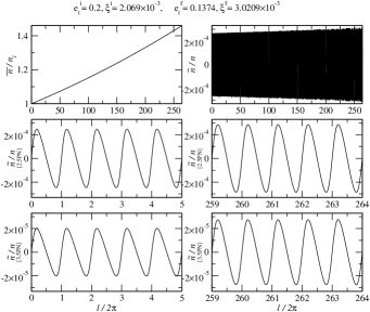
Figure 1: The plots for $\bar{n}/n_{i}$ and $\tilde{n}/n$ versus $l/(2\pi)$, which gives the number of orbital revolutions. The adiabatic increase of $\bar{n}$ is clearly visible in panel 1, and the quasi-periodic nature of the variations in $\tilde{n}$ is portrayed in panels 2–6. These variations are governed by the reactive 2.5PN and 3.5PN equations of motion. In the second and third row, these contributions to $\tilde{n}$ are plotted individually and separated for the initial and final stages. The parameters $e_{t}^{i}$ and $e_{t}^{f}$ denote initial and final values of the time eccentricity $e_{t}$, while $\xi^{i}$ and $\xi^{f}$ stand for similar values of the adimensional mean motion $\xi=GMn/c^{3}$. The panels are plotted for $\eta=0.25$ and the orbital evolution is terminated when $j=\sqrt{48}$.

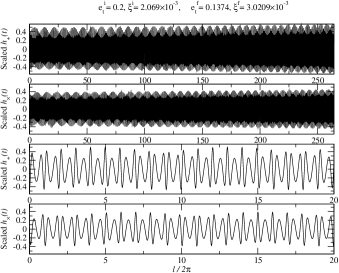
Figure 2: The plots for the scaled $h_{+}(t)$ and $h_{\times}(t)$ (Newtonian in amplitude and 3.5PN in orbital motion) as functions of $l/(2\pi)$. The slow chirping and the amplitude modulation due to the periastron precession are clearly visible in the two upper panels. In the two bottom panels, we zoom into the initial stages of the orbital evolution in order to show the effect of the periodic orbital motion and the periastron advance on the scaled $h_{+}(t)$ and $h_{\times}(t)$. The initial and final values of the relevant orbital elements are marked on top of the plots. The panels are plotted for a binary consisting of equal masses, so that $\eta=0.25$, and the orbital inclination angle is given by $i=\pi/3$. The orbital evolution is terminated when $j=\sqrt{48}$.

In Fig. 1 we plot $\bar{n}/n_{i}$, where $n_{i}$ is the initial value of $n$, and $\tilde{n}/n$, as functions of $l/(2\pi)$, which gives the evolution in terms of elapsed orbital cycles. We clearly see an adiabatic increase of $\bar{n}$ as well as the quasi-periodic variations of $\tilde{n}$. These variations are governed by the reactive 2.5PN and 3.5PN equations of motion. In the second and third row of Fig. 1, these contributions to $\tilde{n}$ are plotted individually and separated for the initial and final stages. These 2.5PN and 3.5PN contributions are obviously in-phase, and we observe that the scaled 3.5PN contributions are only by a factor of $\sim 10$ smaller than their scaled 2.5PN counterparts.

Though, we have all the required computations to plot the secular and quasi-periodic variations in $e_{t}$, $c_{l}$, and $c_{\lambda}$ to the 1PN reactive order, we do not attempt it here. As expected, we observed the same features at the 3.5PN order, as detailed in Figs. 2 and 3 in Ref. DGI at the 2.5PN order — the adiabatic decrease of $\bar{e}_{t}$, the periodic variations of $\tilde{e}_{t}$, no secular evolution of $\bar{c}_{l}$ and $\bar{c}_{\lambda}$, but periodic variations in $\tilde{c}_{l}$ and $\tilde{c}_{\lambda}$ — and that is the main reason for not duplicating these figures.

Finally, we plot in Fig. 2 the scaled $h_{+}(t)$ and $h_{\times}(t)$, evolving under gravitational radiation reaction, as functions of $l/(2\pi)$. [We factored out $G\mu/(c^{4}R^{\prime})$ appearing in $h_{+}|_{\rm Q}$ and $h_{\times}|_{\rm Q}$ to get the scaled waveforms.] We employ for these figures polarization amplitudes, which are Newtonian accurate, as given by Eqs. (3), while the orbital motion is 3.5PN accurate. We clearly see “chirping” due to radiation damping, amplitude modulation due to periastron precession, and also orbital period variations.

We note that Figs. 1 and 2 can be used to illustrate the various aspects of a compact binary inspiral from sources relevant for both LIGO and LISA. This is based on the above mentioned scaling argument. Let us detail this in case of the following two scenarios. For instance, if we choose for the total mass $M=2.8M_{\odot}$ — a binary inspiral involving two $1.4M_{\odot}$ compact objects — the variation of $\xi$ from $2.069\times 10^{-3}$ to $3.0209\times 10^{-3}$ in $\sim 264$ orbital cycles corresponds to a increasing orbital frequency from $150$ Hz to $219$ Hz in $\sim 7.58$ s. Similarly, for the choice of $M=10^{5}M_{\odot}$ — a binary inspiral involving two supermassive black holes — the variation of $\xi$ from $2.069\times 10^{-3}$ to $3.0209\times 10^{-3}$ in $\sim 264$ orbital cycles corresponds to a increasing orbital frequency from $\sim 4.2\times 10^{-3}$ Hz to $\sim 6.1\times 10^{-3}$ Hz in $\sim 3.1$ days.

We conclude by noting that Fig. 1 shows clearly the existence of periodic variations in the orbital elements — analytically investigated for the first time in Ref. DGI and improved to the 3.5PN order in this paper.

V Conclusions

Let us recapitulate. In this paper, we have incorporated the 3PN accurate conservative and the 1PN accurate reactive dynamics in harmonic coordinates into the phasing formalism to the 3.5PN order as a natural extension of the work presented in Ref. DGI . This extension was possible due to the very recent determination of the 3PN accurate generalized quasi-Keplerian parametrization for the conservative orbital motion of nonspinning compact binaries in eccentric orbits MGS . We applied the method of Ref. DGI to construct, almost analytically, templates for GW signals emitted by compact binaries moving in inspiralling and slowly precessing eccentric orbits. An improved method of variation of arbitrary constants, explained in great detail in Ref. DGI , allowed us to combine the three different but relevant time scales, namely, those associated with the radial motion (orbital period), advance of periastron, and radiation reaction, to the 3.5PN order without making the usual approximation of treating adiabatically the radiative time scale. In this context, we recall that the two-scale decomposition helped us to model accurately and efficiently the time evolution of the associated dynamical variables. We employed harmonic coordinates in this paper as calculations that provided search templates for compact binaries in quasi-circular orbits usually employ the harmonic gauge.

The explicit computations provided in this paper will be required to construct accurate and efficient search templates for gravitational waves from compact binaries of arbitrary mass ratio moving in inspiralling eccentric orbits. Our detailed calculations will have to be employed, if the earth-based GW interferometers plan to search for gravitational waves from compact binaries with residual eccentricities, motivated by a plethora of recent astrophysical investigations K62 ; MH02 ; Rasio2000 ; W03 ; DLK05 ; Page05 ; GZM_nature_2006 ; CB05 ; HA05_ApJ ; RS_MNRAS . The proposed space-based GW interferometers like LISA, BBO, and DECIGO will have to depend on our results to do astrophysics. It is interesting to note that our results will be required by LISA to search for gravitational waves from stellar-mass, intermediate-mass, and supermassive black-hole binaries as these binaries will likely to be in inspiralling eccentric orbits. Another area where our computations can be quite effective will be the early stages of extreme mass ratio inspiral (EMRI) as relevant for LISA. Our current results should be also useful to benchmark efforts that are required to obtain reliable EMRI templates Mino2006 .

There are many avenues that will require detailed investigations in the near future and we list only a few of them below. In this paper, the conservative dynamics was restricted to compact binaries consisting of nonspinning point masses. Naturally, it is desirable to include spin effects into our computations. A first step in this direction was taken in Ref. KG05_so_para , where the 3PN accurate generalized quasi-Keplerian parametrization for the conservative dynamics of spinning compact binaries, moving in eccentric orbits, when the spin effects are restricted to the leading-order spin-orbit interaction, is presented. We also neglected, for simplicity, explicit PN corrections to the GW polarization amplitudes of $h_{+}$ and $h_{\times}$, and restricted them to their leading quadrupolar order. However, it is possible to obtain 2PN accurate corrections to these amplitudes, using Refs. DGI ; GI97 . In order to make the numerical implementation of our computations more efficient and accurate, it is also desirable to provide better ways of solving the 3PN accurate Kepler equation. Another line of investigation should deal with a extension of these computations so that we have a dependable description for the orbital evolution near the LSO. Finally, these templates naturally trigger lots of data analysis investigations relevant for both ground-based and space-based GW interferometers. Many of the above mentioned issues are currently under investigation.

Appendix A Construction of an exact relation for $v-u$

In this appendix, we provide the details involved in the derivation of the exact relation for $v-u$, which is also periodic in $u$:

$$v-u =2\tan^{-1}\left(\frac{\beta_{\phi}\sin u}{1-\beta_{\phi}\cos u}\right)\,,$$ (42)

where $\beta_{\phi}=(1-\sqrt{1-e_{\phi}^{2}})/e_{\phi}$. This relation allows us to avoid the usage of the commonly employed infinite series expression for $v-u$, namely,

$$v-u =2\sum_{i=1}^{\infty}\frac{\beta_{\phi}^{i}}{i}\sin iu\,.$$ (43)

In order to deduce Eq. (42), we start from the following identity

$$v-u \equiv 2\tan^{-1}\left[\tan\left(\frac{v-u}{2}\right)\right]\,.$$ (44)

Using therein

$$\tan(\alpha-\beta) =\frac{\tan\alpha-\tan\beta}{1+\tan\alpha\tan\beta}\,,$$ (45)

leads to

$$v-u =2\tan^{-1}\left[\frac{\tan\frac{v}{2}-\tan\frac{u}{2}}{1+\tan\frac{v}{2}\tan\frac{u}{2}}\right]\,.$$ (46)

The relation connecting the true anomaly $v$ to the eccentric anomaly $u$, as given by Eq. (9c), is used to replace $\tan(v/2)$ in the above equation. In this way, we obtain

$$v-u =2\tan^{-1}\left[\frac{(Q_{\phi}-1)\tan\frac{u}{2}}{1+Q_{\phi}\tan^{2}\frac{u}{2}}\right]\,,$$ (47)

where

$$Q_{\phi} =\left(\frac{1+e_{\phi}}{1-e_{\phi}}\right)^{1/2}\,.$$ (48)

With the help of

$$\tan\frac{u}{2} =\frac{\sin u}{1+\cos u}\,,$$ (49)

we rewrite Eq. (47) as

$$v-u =2\tan^{-1}\left[\frac{\frac{Q_{\phi}-1}{Q_{\phi}+1}\sin u}{1-\frac{Q_{\phi}-1}{Q_{\phi}+1}\cos u}\right]\,.$$ (50)

Now, let us call

$$\beta_{\phi} \equiv\frac{Q_{\phi}-1}{Q_{\phi}+1}\,,$$ (51)

which can be simplified to

$$\beta_{\phi} =\frac{1-\sqrt{1-e_{\phi}^{2}}}{e_{\phi}}\,.$$ (52)

Finally, the combination of Eqs. (50)–(52) directly leads to Eq. (42).

In addition, analog to the above derivation, we constructed the following exact relation, involving the time eccentricity $e_{t}$ instead of $e_{\phi}$,

$$2\tan^{-1}\left[\left(\frac{1+e_{t}}{1-e_{t}}\right)^{1/2}\tan\frac{u}{2}\right]-u\\ =2\tan^{-1}\left(\frac{\beta_{t}\sin u}{1-\beta_{t}\cos u}\right)\,,$$ (53)

where $\beta_{t}=(1-\sqrt{1-e_{t}^{2}})/e_{t}$, which was required in case of Eqs. (36) and (36).

Appendix B 2PN accurate adiabatic evolution of $\bar{n}$ and $\bar{e}_{t}$ in harmonic coordinates

Following Ref. DGI , let us briefly show in this appendix how to obtain, in harmonic coordinates, the 2PN accurate secular changes in $\bar{n}$ and $\bar{e}_{t}$. The PN accurate differential equations for $\bar{n}$ and $\bar{e}_{t}$ are computed using the heuristic arguments, detailed in Ref. BS1989 and in Sec. VI in Ref. DGI . In the heuristic determination of the evolution equations for $\bar{n}$ and $\bar{e}_{t}$, one employs PN accurate expressions for $n$ and $e_{t}$, and the far-zone (FZ) energy and angular-momentum fluxes. The PN accurate expressions for $d\bar{n}/dt$ and $d\bar{e}_{t}/dt$ are then obtained by differentiating the PN accurate expressions for $n$ and $e_{t}$, expressed in terms of $E$ and $L$, with respect to time and then heuristically equating the resulting time derivatives of $E$ and $L$ to the orbital averaged expressions for the FZ energy and angular-momentum fluxes. For the ease of implementation, we split the 2PN accurate computations of $d\bar{n}/dt$ and $d\bar{e}_{t}/dt$ into two parts. The first part contains the purely “instantaneous” 2PN corrections and the second part considers the so-called “tail” contributions Def_Inst , appearing at the 1.5PN (reactive) order and derived for the first time in Refs. BS1993 ; RS97 . The computations to get the instantaneous contributions begin with the 2PN corrections to the FZ fluxes, in harmonic gauge, in terms of $r$, $\dot{r}$, and $v^{2}$ available in Ref. GI97 . These FZ fluxes are orbital averaged, using the 2PN accurate generalized quasi-Keplerian parametrization for elliptical orbits in harmonic gauge, following the prescripton detailed in Ref. BS1989 . We perform the orbital average by using an additional ingredient, namely, the relation connecting $dl$ and $du$ to 2PN order in harmonic coordinates

$$\frac{dl}{du} =\chi+\frac{\xi^{4/3}}{8\chi^{2}\sqrt{1-e_{t}^{2}}}\bigg{[}(15\eta-\eta^{2})(1-e_{t}^{2})^{3/2}$$

$$\quad+(60-39\eta+\eta^{2})\chi\sqrt{1-e_{t}^{2}}-(60-24\eta)\chi^{2}\bigg{]}\,,$$ (54)

where $\chi=1-e_{t}\cos u$. The resulting definite integrals are easily computed, using Eq. (31). Now, we compute the time derivatives of the PN accurate expressions for $n$ and $e_{t}$ and equate the resulting time derivatives of $E$ and $L$ to the orbital averaged expressions for the FZ energy and angular-momentum fluxes, respectively, to get the PN accurate expressions for $d\bar{n}/dt$ and $d\bar{e}_{t}/dt$ in terms of $E$, $L$, $M$, and $\eta$. Finally, we use Eqs. (21) to obtain the differential equations for $\bar{n}$ and $\bar{e}_{t}$ in terms of $\bar{n}$, $\bar{e}_{t}$, $M$, and $\eta$. The resulting 2PN accurate instantaneous contributions to $d\bar{n}/dt$ and $d\bar{e}_{t}/dt$, in harmonic coordinates, are given by

$$\frac{d\bar{n}}{dt} =\bar{\xi}^{5/3}\bar{n}^{2}\eta\left\{\dot{\bar{n}}^{\rm N}+\dot{\bar{n}}^{\rm 1PN}+\dot{\bar{n}}^{\rm 2PN}\right\}\,,$$ (55a)

$$\frac{d\bar{e}_{t}}{dt} =-{\bar{\xi}}^{5/3}\bar{n}\eta\bar{e}_{t}\left\{\dot{\bar{e}}_{t}^{\rm N}+\dot{\bar{e}}_{t}^{\rm 1PN}+\dot{\bar{e}}_{t}^{\rm 2PN}\right\}\,,$$ (55b)

where the various instantaneous PN accurate corrections, namely, $\dot{\bar{n}}^{\rm N}$, $\dot{\bar{n}}^{\rm 1PN}$, $\dot{\bar{n}}^{\rm 2PN}$, $\dot{\bar{e}}_{t}^{\rm N}$, $\dot{\bar{e}}_{t}^{\rm 1PN}$, and $\dot{\bar{e}}_{t}^{\rm 2PN}$, read

$$\dot{\bar{n}}^{\rm N} =\frac{1}{5(1-\bar{e}_{t}^{2})^{7/2}}\Bigl{\{}96+292\bar{e}_{t}^{2}+37\bar{e}_{t}^{4}\Bigr{\}}\,,$$ (56a)

$$\dot{\bar{n}}^{\rm 1PN} =\frac{\bar{\xi}^{2/3}}{280(1-\bar{e}_{t}^{2})^{9/2}}\Bigl{\{}20368-14784\eta+(219880-159600\eta)\bar{e}_{t}^{2}+(197022-141708\eta)\bar{e}_{t}^{4}+(11717-8288\eta)\bar{e}_{t}^{6}\Bigr{\}}\,,$$ (56b)

$$\dot{\bar{n}}^{\rm 2PN} =\frac{\bar{\xi}^{4/3}}{30240(1-\bar{e}_{t}^{2})^{11/2}}\Bigl{\{}12592864-13677408\eta+1903104\eta^{2}+(133049696-185538528\eta+61282032\eta^{2})\bar{e}_{t}^{2}$$

$$\quad+(284496744-411892776\eta+166506060\eta^{2})\bar{e}_{t}^{4}+(112598442-142089066\eta+64828848\eta^{2})\bar{e}_{t}^{6}$$

$$\quad+(3523113-3259980\eta+1964256\eta^{2})\bar{e}_{t}^{8}+3024(96+4268\bar{e}_{t}^{2}+4386\bar{e}_{t}^{4}+175\bar{e}_{t}^{6})(5-2\eta)\sqrt{1-\bar{e}_{t}^{2}}\Bigr{\}}\,,$$ (56c)

$$\dot{\bar{e}}_{t}^{\rm N} =\frac{1}{15(1-\bar{e}_{t}^{2})^{5/2}}\Bigl{\{}304+121\bar{e}_{t}^{2}\Bigr{\}}\,,$$ (56d)

$$\dot{\bar{e}}_{t}^{\rm 1PN} =\frac{\bar{\xi}^{2/3}}{2520(1-\bar{e}_{t}^{2})^{7/2}}\Bigl{\{}340968-228704\eta+(880632-651252\eta)\bar{e}_{t}^{2}+(125361-93184\eta)\bar{e}_{t}^{4}\Bigr{\}}\,,$$ (56e)

$$\dot{\bar{e}}_{t}^{\rm 2PN} =\frac{\bar{\xi}^{4/3}}{30240(1-\bar{e}_{t}^{2})^{9/2}}\Bigl{\{}20815216-25375248\eta+4548096\eta^{2}+(87568332-128909916\eta+48711348\eta^{2})\bar{e}_{t}^{2}$$

$$\quad+(69916862-93522570\eta+42810096\eta^{2})\bar{e}_{t}^{4}+(3786543-4344852\eta+2758560\eta^{2})\bar{e}_{t}^{6}$$

$$\quad+1008(2672+6963\bar{e}_{t}^{2}+565\bar{e}_{t}^{4})(5-2\eta)\sqrt{1-\bar{e}_{t}^{2}}\Bigr{\}}\,,$$ (56f)

where $\bar{\xi}\equiv GM\bar{n}/c^{3}$. The tail contributions to $d\bar{n}/dt$ and $d\bar{e}_{t}/dt$, which appear at the 1.5PN order, are already presented in Sec. VI in Ref. DGI , given by Eqs. (70) and (71) therein.

We have checked that to the 1PN order the above contributions are in excellent agreement with Eqs. (68) and (69) in Ref. DGI , which give the instantaneous 2PN accurate contributions to $d\bar{n}/dt$ and $d\bar{e}_{t}/dt$ in ADM gauge. Note also the expected differences at higher-PN orders between the harmonic and the ADM gauge. We conclude by noting that the article providing the 3PN accurate contributions to $d\bar{n}/dt$ and $d\bar{e}_{t}/dt$ is currently under preparation Bala_private .

References

- (1) Following URLs provide a wealth of information about the terrestrial GW interferometers: http://www.ligo.caltech.edu, http://www.virgo.infn.it, http://www.geo600.uni-hannover.de, and http://tamago.mtk.nao.ac.jp.
- (2) L. Blanchet, T. Damour, G. Esposito-Farèse, and B. R. Iyer, Phys. Rev. D 71, 124004 (2005); Phys. Rev. Lett. 93, 091101 (2004); L. Blanchet, T. Damour, and G. Esposito-Farèse, Phys. Rev. D 69, 124007 (2004); L. Blanchet, G. Faye, B. R. Iyer, and B. Joguet, Phys. Rev. D 65, 061501(R) (2002); 71, 129903(E) (2005); T. Damour, P. Jaranowski, and G. Schäfer, Phys. Lett. B 513, 147 (2001).
- (3) K. G. Arun, L. Blanchet, B. R. Iyer, and M. S. S. Qusailah, Class. Quant. Grav. 21, 3771 (2004); 22, 3115(E) (2005).
- (4) Y. Kozai, Astron. J. 67, 591 (1962).
- (5) M. C. Miller and D. P. Hamilton, Astrophys. J. 576, 894 (2002).
- (6) E. B. Ford, B. Kozinsky, and F. A. Rasio, Astrophys. J. 535, 385 (2000); 605, 966(E) (2004).
- (7) L. Wen, Astrophys. J. 598, 419 (2003).
- (8) M. B. Davies, A. J. Levan, and A. R. King, Mon. Not. R. Astron. Soc. 356, 54 (2005).
- (9) K. L. Page et al., Astrophys. J. 637, L13 (2006).
- (10) J. Grindlay, S. P. Zwart, and S. McMillan, Nature (London) 2, 116 (2006).
- (11) H. K. Chaurasia and M. Bailes, Astrophys. J. 632, 1054 (2005).
- (12) C. Hopman and T. Alexander, Astrophys. J. 629, 362 (2005).
- (13) G. Kupi, P. Amaro-Seoane, and R. Spurzem, Dynamics of compact objects: A post-Newtonian study, submitted to MNRAS, astro-ph/0602125.
- (14) http://lisa.jpl.nasa.gov.
- (15) E. S. Phinney et al., The Big Bang Observer: Direct detection of gravitational waves from the birth of the Universe to the Present, NASA Mission Concept Study (2004).
- (16) N. Seto, S. Kawamura, and T. Nakamura, Phys. Rev. Lett. 87, 221103 (2001).
- (17) K. Gültekin, M. C. Miller, and D. P. Hamilton, Three-Body Dynamics with Gravitational Wave Emission, accepted for publication in ApJ, astro-ph/0509885.
- (18) T. Matsubayashi, J. Makino, and T. Ebisuzaki, Evolution of Galactic Nuclei. I. orbital evolution of IMBH, submitted to ApJ, astro-ph/0511782.
- (19) M. A. Gürkan, J. M. Fregeau, and F. A. Rasio, Massive Black Hole Binaries from Collisional Runaways, accepted for publication in ApJ Letters, astro-ph/0512642.
- (20) S. J. Aarseth, Astrophysics and Space Science 285, 367 (2003).
- (21) P. Berczik, D. Merritt, R. Spurzem, and H.-P. Bischof, Efficient Merger of Binary Supermassive Black Holes in Non-Axisymmetric Galaxies, astro-ph/0601698.
- (22) O. Blaes, M. H. Lee, and A. Socrates, Astrophys. J. 578, 775 (2002).
- (23) P. J. Armitage and P. Natarajan, Astrophys. J. 634, 921 (2005).
- (24) M. Iwasawa, Y. Funato, and J. Makino, Evolution of Massive Blackhole Triples I — Equal-mass binary-single systems, astro-ph/0511391.
- (25) T. Damour, A. Gopakumar, and B. R. Iyer, Phys. Rev. D 70, 064028 (2004).
- (26) T. Damour, in Gravitational Radiation, edited by N. Deruelle and T. Piran (North-Holland, Amsterdam, 1983).
- (27) T. Damour, Phys. Rev. Lett. 51, 1019 (1983).
- (28) T. Damour, in Proceedings of Journées Relativistes 1983, edited by S. Benenti, M. Ferraris, and M. Francaviglia (Pitagora Editrice, Bologna, 1985), pp. 89–110.
- (29) T. Damour and N. Deruelle, Ann. Inst. Henri Poincaré Phys. Théor. 44, 263 (1986).
- (30) T. Damour and J. Taylor, Phys. Rev. D 45, 1840 (1992).
- (31) R.-M. Memmesheimer, A. Gopakumar, and G. Schäfer, Phys. Rev. D 70, 104011 (2004).
- (32) P. Jaranowski and G. Schäfer, Phys. Rev. D 57, 7274 (1998); 60, 124003 (1999); T. Damour, P. Jaranowski, and G. Schäfer, Phys. Rev. D 62, 021501(R) (2000); 63, 029903(E) (2001); 63, 044021 (2001); 66, 029901(E) (2002); Phys. Lett. B 513, 147 (2001).
- (33) L. Blanchet and G. Faye, Phys. Lett. A 271, 58 (2000); Phys. Rev. D 63, 062005 (2000); J. Math. Phys. (N.Y.) 41, 7675 (2000); 42, 4391 (2001).
- (34) A. Gopakumar and C. Königsdörffer, Phys. Rev. D 72, 121501(R) (2005).
- (35) T. Damour and N. Deruelle, Ann. Inst. Henri Poincare Phys. Theor. 43, 107 (1985).
- (36) T. Damour and G. Schäfer, Nuovo Cimento Soc. Ital. Fis., B 101, 127 (1988).
- (37) G. Schäfer and N. Wex, Phys. Lett. A 174, 196 (1993); 177, 461(E) (1993).
- (38) L. Blanchet, T. Damour, B. R. Iyer, C. M. Will, and A. G. Wiseman, Phys. Rev. Lett. 74, 3515 (1995); L. Blanchet, T. Damour, and B. R. Iyer, Phys. Rev. D 51, 5360 (1995).
- (39) L. Blanchet, B. R. Iyer, C. M. Will, and A. G. Wiseman, Class. Quant. Grav. 13, 575 (1996).
- (40) C. M. Will and A. G. Wiseman, Phys. Rev. D 54, 4813 (1996).
- (41) A. Gopakumar and B. R. Iyer, Phys. Rev. D 56, 7708 (1997).
- (42) L. Blanchet and B. R. Iyer, Class. Quant. Grav. 20, 755 (2003).
- (43) C. Königsdörffer and A. Gopakumar, Phys. Rev. D 71, 024039 (2005).
- (44) C. Königsdörffer and A. Gopakumar, Phys. Rev. D 73, 044011 (2006).
- (45) T. Damour, P. Jaranowski, and G. Schäfer, Phys. Rev. D 62, 044024 (2000).
- (46) M. E. Pati and C. M. Will, Phys. Rev. D 65, 104008 (2002); S. Nissanke and L. Blanchet, Class. Quant. Grav. 22, 1007 (2005); The corresponding resuts in ADM gauge are given in C. Königsdörffer, G. Faye, and G. Schäfer, Phys. Rev. D 68, 044004 (2003).
- (47) W. H. Whittaker and G. N. Watson, Modern Analysis, (Cambridge University, Cambridge, 1927).
- (48) L. Blanchet and G. Schäfer, Mon. Not. R. Astron. Soc. 239, 845 (1989).
- (49) W. Junker and G. Schäfer, Mon. Not. R. Astron. Soc. 254, 146 (1992).
- (50) Y. Mino, Adiabatic Expansion for Metric Perturbation and the condition to solve the Gauge Problem for Gravitational Radiation Reaction Problem, accepted for publication in Progress of Theoretical Physics, gr-qc/0601019.
- (51) Following Ref. BDIWW , we term contributions to the GW amplitude and its associated quantities that depend only on the state of the binary at the retarded instant as its “instantaneous” part, whereas the contributions, which are a priori sensitive to the entire “history” of the binary’s dynamics are termed as the “tail” contributions.
- (52) L. Blanchet and G. Schäfer, Class. Quant. Grav. 10, 2699 (1993).
- (53) R. Rieth and G. Schäfer, Class. Quant. Grav. 14, 2357 (1997).
- (54) K. G. Arun, L. Blanchet, B. R. Iyer, and M. S. S. Qusailah, to be published.