A simple accretion model of a rotating gas sphere onto a Schwarzschild black hole

Abstract

We construct a simple accretion model of a rotating gas sphere onto a Schwarzschild black hole. We show how to build analytic solutions in terms of Jacobi elliptic functions. This construction represents a general relativistic generalisation of the Newtonian accretion model first proposed by Ulrich (1976). In exactly the same form as it occurs for the Newtonian case, the flow naturally predicts the existence of an equatorial rotating accretion disc about the hole. However, the radius of the disc increases monotonically without limit as the flow reaches its minimum allowed angular momentum for this particular model.

1 Introduction

Steady spherically symmetric accretion onto a central gravitational potential (e.g. a star) was first investigated by Bondi (1952). This pioneering work turned out to have many different applications to astrophysical phenomena (see e.g. Frank et al. (2002)), despite of the fact that it was only constructed for curiosity, rather than a realistic idea to a particular astrophysical situation (Bondi, 2005). A general relativistic generalisation to the work of Bondi was made by Michel (1972). Both models can be seen as astrophysical examples of transonic flows that naturally occur in the Universe.

Realistic models of spherical accretion require an extra ingredient that seems inevitable in many astronomical situations. This is so because gas clouds, where compact objects are embedded, have a certain degree of rotation. This rotation enables the formation of an equatorial accretion disc for which gas particles rotate about the central object. The first steady accretion model, in which a rotating gas sphere with infinite extent is accreted to a central object was first investigated by Ulrich (1976). In his model, Ulrich considered a gas cloud rotating as a rigid body and took no account of pressure gradients associated to the infalling gas. In other words, his analysis is approximately ballistic. For, the the initial specific angular momentum of an infalling particle is small and heating by radiation as well as viscosity effects are negligible. In addition, pressure gradients and internal energy changes along the streamlines of a supersonic flow provide negligible contributions to the momentum and energy balances respectively (cf. Ulrich, 1976; Cassen & Moosman, 1981; Mendoza et al., 2004).

A first order general relativistic approximation of a rotating gas sphere was made by Beloborodov & Illarionov (2001). In their model, they used approximate solutions for the integration of the geodesic equation and their boundary conditions are such that the specific angular momentum for a single particle $h\leq 2r_{\text{g}}$, where $r_{\text{g}}$ is the Schwarzschild radius. In here and in what follows we use a system of units for which $G=c=1$, where $G$ is the gravitational constant and $c$ the speed of light. In this article we show that such a model is not a general relativistic Ulrich flow, since its appropriate generalisation must satisfy the inequality $h\geq 2r_{\text{g}}$. A pseudo–Newtonian Paczynsky & Wiita (1980) numerical approximation of the extreme hyperbolic $h=2r_{\text{g}}$ case was discussed by Lee & Ramirez-Ruiz (2006). We show that this pseudo–Newtonian numerical approach differs in a significant way when compared with the complete general relativistic solution.

In this article we develop a full general relativistic model of a rotating gas sphere of infinite extent that accretes matter onto a centrally symmetric Schwarzschild space–time. We assume that heating by radiation and viscosity effects are small so that the flow can be treated as ideal. Since pressure gradients and internal energy changes along the streamlines of a supersonic flow provide negligible contributions to the momentum and energy balances respectively, the flow is well approximated by ballistic trajectories. We also assume that the self–gravity of the accreting gas does not change the structure of the Schwarzschild space–time. This is of course true if the mass of the central object that shapes the space–time is much greater than the mass of the rotating cloud. With these assumptions, we find velocity and particle number density fields as well as the streamlines of the flow in an exact analytic form using Jacobi Elliptic functions. The remaining thermodynamic quantities are easily found by assuming a polytropic flow, for which the pressure is proportional to a power of the particle number density (see for e.g. Stanyukovich, 1960). In section 2 we state the main results from general relativity used to solve the model introduced in section 3. We show in section 4 that the general solution converges to the accretion model considered by Ulrich (1976) and that for the case of a null value for the specific angular momentum, the velocity field converges to the one described by Michel (1972) for a null value of the pressure gradients on the fluid. The particular case of a minimum specific angular momentum $h=2r_{\text{g}}$ is calculated in section 5, and it is shown that the solutions can be found with the aid of simple hyperbolic functions. Finally, in section 6 we discuss the physical consequences implied by this general relativistic model.

2 Background in celestial mechanics for general relativity

The main results from relativistic gravity to be used throughout the article are stated in this section. The reader is referred to the general relativity textbooks by Misner et al. (1973); Chandrasekhar (1983); Landau & Lifshitz (1994a); Novikov & Frolov (1990) and Wald (1984) for further details.

It is well known that the vacuum Schwarzschild solution describing the final product of gravitational collapse contains a singularity which is hidden by a horizon. The solution corresponding to an exterior gravitational field of static, spherically symmetric body is given by the Schwarzschild metric:

$$\mathrm{d}s^{2}=-\left(1-\frac{2M}{r}\right)\mathrm{d}t^{2}+\left(1-\frac{2M}{r}\right)^{-1}\mathrm{d}r^{2}+r^{2}\mathrm{d}\Omega^{2},$$ (1)

where $\mathrm{d}\Omega^{2}=\mathrm{d}\theta^{2}+\sin^{2}\theta\,\mathrm{d}\varphi^{2}$ represents the square of an angular displacement. The total mass of the Schwarzschild field is represented by $M$. The temporal, radial, polar and azimuthal coordinates are represented respectively by t, r, $\theta$ and $\varphi$. In equation (1), we have chosen a signature $(-,+,+,+)$ for the metric. In what follows, Greek indices such as $\alpha$, $\beta$, etc., are used to denote space–time components, taking values $0,\ 1,\ 2$ and $3$.

Birkhoff (1923) showed that it is possible to solve the vacuum Einstein field equations for a general spherically symmetric space–time, without the static field assumption. It follows from his calculations that the Schwarzschild solution remains the only solution of this more general space–time.

The behaviour of light rays and test bodies in the exterior gravitational field of a spherical body is described by analysing both, timelike and null geodesics. In order to do that, we first note that the Schwarzschild metric has a parity reflection symmetry, i.e. the transformation $\theta\rightarrow\pi-\theta$ leaves the metric unchanged. Under these considerations it follows that if the initial position and tangent vector of a geodesic lies in the equatorial plane $\theta=\pi/2$, then the entire geodesic must lie in that particular plane. Every geodesic can be brought to an initially equatorial plane by a rotational isometry and so, without loss of generality, it is possible to restrict our attention to the study of equatorial geodesics only.

In what follows we denote the coordinate basis components by $x^{\mu}$ and the tangent vector to a curve by $u^{\alpha}=\mathrm{d}x^{\alpha}/\mathrm{d}\tau$. For timelike geodesics the parameter $\tau$ can be made to coincide with the proper time and for null geodesics it only represents an affine parameter. Under the above circumstances, the geodesics take the following form (cf. Wald (1984)):

$$-\kappa=\ g_{\alpha\beta}\,u^{\alpha}u^{\beta}=-\left(1-\frac{2M}{r}\right)\dot{t}^{2}+\left(1-\frac{2M}{r}\right)^{-1}\dot{r}^{2}+r^{2}\dot{\varphi}^{2},$$ (2)

where

$$\kappa:=\left\{\begin{array}[]{ll}1&\text{for timelike geodesics,}\\ 0&\text{for null geodesics.}\end{array}\right.$$

In the derivation of the geodesic equation (2), there are two important constants of motion that must be taken into account. The first of them is

$$E:=-g_{\alpha\beta}\,\xi^{\alpha}u^{\beta}=\left(1-\frac{2M}{r}\right)\frac{\mathrm{d}t}{\mathrm{d}\tau},$$ (3)

where $\xi^{\alpha}$ represents the static Killing vector and $E$ is a constant of motion. For timelike geodesics $E$ represents the specific energy of a single particle following a given geodesic, relative to a static observer at infinity.

The second constant of motion $h$ is related to the rotational Killing field $\psi^{\alpha}$ by the following relation:

$$h:=g_{\alpha\beta}\psi^{\alpha}u^{\beta}=r^{2}\sin^{2}\theta\frac{\mathrm{d}\varphi}{\mathrm{d}\tau}.$$ (4)

Since we have chosen $\theta=\pi/2$ without loss of generalisation, the previous equation takes the form

$$h=r^{2}\frac{\mathrm{d}\varphi}{\mathrm{d}\tau}.$$ (5)

For timelike geodesics $h$ is the specific angular momentum. The final equation for the geodesics is found by direct substitution of equations (3) and (5) into relation (2). From now on, we restrict the analysis to timelike geodesics only and so, the equation of motion takes the following form:

$$\left(\frac{\mathrm{d}r}{\mathrm{d}\tau}\right)^{2}+\left(1-\frac{2M}{r}\right)\left(1+\frac{h^{2}}{r^{2}}\right)=E^{2}.$$ (6)

This equation shows that the radial motion of a geodesic is very similar to that of a unit mass particle of energy $E^{2}$ in ordinary one dimensional non-relativistic mechanics. The feature provided by general relativity in equation (6) is that, apart from a Newtonian gravitational term $-2M/r$ and the centrifugal barrier $h^{2}/r^{2}$, there is a new attractive potential term $-2Mh^{2}/r^{3}$, that dominates over the centrifugal barrier for sufficiently small $r$.

As it is done in the analysis of the Keplerian orbit for Newtonian gravity (see for example Landau & Lifshitz (1994b)), it is useful to consider $r$ as a function of $\varphi$ instead of $\tau$. Therefore, equation (6) takes the form

$$\left(\frac{\mathrm{d}r}{\mathrm{d}\varphi}\right)^{2}=\frac{2Mr^{3}}{h^{2}}-r^{2}+2Mr+\left(E^{2}-1\right)\left(\frac{r^{4}}{h^{2}}\right).$$ (7)

Now, letting $E^{2}-1:=2E_{\text{tot}}$, where $E_{\text{tot}}$ is the total energy of the particle and $u=r^{-1}$ equation (7) takes the final form

$$\left(\frac{\mathrm{d}u}{\mathrm{d}\varphi}\right)^{2}=2Mu^{3}-u^{2}+\frac{2Mu}{h^{2}}+\frac{2E_{\text{tot}}}{h^{2}}.$$ (8)

Let us define $u:=Mv/h^{2}$ so that the previous equation simplifies to

$$\left(\frac{\mathrm{d}v}{\mathrm{d}\phi}\right)^{2}=\alpha v^{3}-v^{2}+2v+\epsilon,$$ (9)

where

$$\alpha:=2\left(\frac{M}{h}\right)^{2},\qquad\epsilon:=\frac{2E_{\text{tot}}h^{2}}{M^{2}}.$$ (10)

This equation determines the geometry of the geodesics on the invariant plane labelled by $\theta=\pi/2$. In fact, this equation governs the geometry of the orbits described on the invariant plane due to the fact that the geometry of the geodesics is determined by the roots of the cubic equation

$$f(v)=\alpha v^{3}-v^{2}+2v+\epsilon.$$ (11)

The parameter $\alpha$ provides the difference between the general relativistic and the Newtonian case. In fact, $\alpha\rightarrow 0$ in the Newtonian limit. Finally, the eccentricity $\boldsymbol{e}$ of the Newtonian orbit is related to $\epsilon$ through the relation

$$\boldsymbol{e}^{2}=1+\epsilon.$$

3 Accretion model

The model first proposed by Ulrich (1976) describes a non–relativistic steady accretion flow that considers a central object for which fluid particles fall onto it due to its gravitational potential. Their initial angular momentum $h_{\infty}$ at infinity is considered small in such a way that this model is a small perturbation of Bondi (1952)’s spherical accretion model. The specific initial conditions far away from the origin combined with the assumption that radiative processes and viscosity play no important role on the flow, imply that the streamlines have a parabolic shape. When fluid particles arrive at the equator they thermalise their velocity component normal to the equator. Since the angular momentum for a particular fluid particle is conserved, it follows that particles orbit about the central object once they reach the equator. The radius $r_{\text{dN}}$ of the Newtonian accretion disc, where particles orbit about the central object, is given by (Ulrich, 1976; Mendoza et al., 2004)

$$r_{\text{dN}}=h_{\infty}^{2}/M.$$ (12)

The velocity field and the density profiles are calculated by energy and mass conservation arguments.

We consider now a general relativistic Ulrich situation in which rotating fluid particles fall onto a central object that generates a Schwarzschild space–time. As described in section 1, our analysis is well described by a ballistic approximation. The equation of motion for each fluid particle is thus described by relation (9).

In order to get quantitative results it is important to establish the boundary conditions at infinity. The angular momentum is given by equation (5), so if a particle that falls onto the black hole has an initial velocity $v_{0}$ at an initial polar angle $\theta_{0}$ and the radial distance between the particle and the black hole is $r_{0}$, then the angular momentum is given by

$$h_{\infty*}=r_{0}^{2}\frac{\mathrm{d}\varphi}{\mathrm{d}\tau}=r_{0}\,\gamma_{0}\,v_{0}\,\sin\theta_{0},$$ (13)

where $\gamma_{0}:=\left(1-v_{0}^{2}\right)^{-1/2}$ is the Lorentz factor for the velocity $v_{0}$.

In addition, $h_{\infty*}$ is related to the angular momentum $h$ perpendicular to the invariant plane through the relation

$$h=h_{\infty*}\sin\theta_{0}.$$ (14)

In the Newtonian case, the specific angular momentum $h_{\infty*}$ converges to the value calculated by Ulrich (1976).

With the above relations it is then possible to calculate the equation for a given fluid particle falling onto the central object. First of all, equation (11) states that, if $f(v)$ is a cubic polynomial in $v$, then either all of its roots are real or one of them is real and the two remaining are a complex–conjugate pair. The fact that the particle’s energy is insufficient to permit its escape from the black hole’s gravitational field requires that $\epsilon<0$. This implies that the roots $v_{1},\ v_{2},\$ and $v_{3}$ of $f(v)$ are all real and satisfy the inequality $v_{1}<v_{2}<v_{3}$. Thus, $f(v)$ can be written as

$$f(v)=\alpha\left(v-v_{1}\right)\left(v_{2}-v\right)\left(v_{3}-v\right).$$ (15)

Direct substitution of this relation in equation (9) yields the integration

$$-\frac{2}{\left[\left(v_{2}-v_{1}\right)\left(v_{3}-v_{1}\right)\right]^{1/2}}\int\frac{\mathrm{d}w}{\left[\left(w^{2}-w_{1}^{2}\right)\left(w^{2}-w_{2}^{2}\right)\right]^{1/2}}=\alpha^{1/2}\varphi,$$ (16)

where $w_{1}^{2}=1/\left(v_{2}-v_{1}\right)$, $w_{2}^{2}=1/\left(v_{3}-v_{1}\right)$ and $v=v_{1}+w^{-2}$. This elliptic integral can be calculated in terms of Jacobi elliptic functions (see for example Cayley (1961); Hancock (1917)) yielding the following result

$$\frac{1}{\left(v_{3}-v_{1}\right)^{1/2}}\text{ns}^{-1}\left\{w\left(v_{2}-v_{1}\right)^{1/2}\right\}=\alpha^{1/2}\varphi.$$ (17)

The modulus $k$ of the Jacobi elliptic function for this particular problem is given by

$$k^{2}=\frac{v_{2}-v_{1}}{v_{3}-v_{1}}.$$ (18)

With the aid of relation (17), the equation of the orbit is now obtained:

$$v=v_{1}+\left(v_{2}-v_{1}\right)\ \text{sn}^{2}\Big{\{}\frac{\varphi}{2}\left[\alpha\left(v_{3}-v_{1}\right)\right]^{1/2}\Big{\}}.$$ (19)

This is a general equation for the orbit. For the particular case we are interested in, it must resemble the orbit proposed by Ulrich when $\alpha=0$. Thus, the equation of the orbit must converge to a parabola in this limit. This is possible if and only if the eccentricity $\boldsymbol{e}=1$, which in turn implies $\epsilon=0$. All these conditions mean that the roots of equation (10) are given by

$$v_{1}=0,\quad v_{2}=\frac{1-\left(1-8\alpha\right)^{1/2}}{2\alpha},\quad v_{3}=\frac{1+\left(1-8\alpha\right)^{1/2}}{2\alpha},$$ (20)

and so, the modulus $k$ of the Jacobi elliptic functions in equation (18) takes the form

$$k^{2}=\frac{1-(1-8\alpha)^{1/2}}{1+(1-8\alpha)^{1/2}}.$$ (21)

Note that the previous equations restrict the value of $\alpha$ in such a way that

$$0\leq\alpha\leq 1/8.$$ (22)

When $\alpha=0$, Ulrich solutions are obtained and the case $\alpha=1/8$ corresponds to the case for which the angular momentum $h=4M=2r_{\text{g}}$ reaches a minimum value.

The orbit followed by a single particle falling onto a Schwarzschild black hole with the Ulrich prescription is then given by

$$v=\frac{p}{r}=v_{2}\,\text{sn}^{2}\varphi\beta,$$ (23)

where

$$\beta:=\frac{\left(\alpha v_{3}\right)^{1/2}}{2}=\left(\frac{1+\left(1-8\alpha\right)^{1/2}}{8}\right)^{1/2},\quad p:=\frac{h^{2}}{M}=\frac{h^{2}_{\infty*}}{M}\sin^{2}\theta_{0}=r_{*}\sin^{2}\theta_{0},$$ (24)

and $p$ is the latus rectum of the generalised conic. Note that in the Newtonian limit, the length $r_{*}$ defined by equation (24) converges to the radius of the Newtonian disc $r_{\text{dN}}$ as shown by relation (12).

Before using the equation of the orbit to find out the velocity field and the particle number density, it is useful to mention some important properties of the Jacobi elliptic functions, such as (Cayley, 1961; Hancock, 1917)

$$\text{sn}^{2}(z,k)+\text{cn}^{2}(z,k)=1$$

$$\text{sn}(z,k)\rightarrow\sin(z),\quad\text{cn}(z,k)\rightarrow\cos(z),\quad\text{dn}(z,k)\rightarrow 1,\quad\text{as}\quad k\rightarrow 0,$$

$$\frac{\mathrm{d}}{\mathrm{d}z}\text{sn}(z,k)=\text{cn}(z,k)\ \text{dn}(z,k),\qquad\frac{\mathrm{d}}{\mathrm{d}z}\text{cn}(z,k)=-\text{sn}(z,k)\ \text{dn}(z,k).$$ (25)

The relativistic conic equation is obtained by direct substitution of these relations onto equation (23), giving

$$r=\frac{p}{v_{2}\left(1-\text{cn}^{2}\varphi\beta\right)}.$$ (26)

This orbit lies on the invariant plane $\theta=\pi/2$. We now obtain an equation of motion in terms of the polar coordinate $\theta$ and the initial polar angle $\theta_{0}$ made by a particle when it starts falling onto the black hole. To do so, we note the fact that in order to recover the geometry of the spherical 3D space as $\alpha\rightarrow 0$ it should be fulfilled that

$$\text{cn}^{2}\varphi\beta=\frac{\text{cn}^{2}\theta_{0}\beta+\text{cn}^{2}\theta\beta-1}{2\text{cn}^{2}\theta_{0}\beta-1}.$$ (27)

Since the invariant plane passes through the origin of coordinates, then the radial coordinate $r$ remains the same if another plane is taken instead of the invariant one. Therefore, the angle $\theta_{0}$ is the same as the one related to the value of the angular momentum of the particle at infinity (cf. equation (13)). Thus, the equation of the orbit is found by direct substitution of equations (13) and (27) into (26), and is given by

$$r=\frac{r_{*}\sin^{2}\theta_{0}\left(2\,\text{cn}^{2}\theta_{0}\beta-1\right)}{v_{2}\left(\text{cn}^{2}\theta_{0}\beta-\text{cn}^{2}\theta\beta\right)}.$$ (28)

In order to work with dimensionless variables, let us make the following transformations

$$\frac{r}{r_{*}}\rightarrow r,\qquad\frac{v_{i}}{v_{\text{k}}}\rightarrow v_{i}\qquad(i=r,\ \theta,\ \varphi),\qquad\frac{n}{n_{0}}\rightarrow n,$$

where

$$v_{i}:=\frac{\mathrm{d}x^{i}}{\mathrm{d}\tau},\qquad n_{0}:=\frac{\dot{M}}{4\pi v_{\text{k}}r^{2}_{*}},\qquad v_{\text{k}}:=\left(\frac{M}{r_{*}}\right)^{1/2}.$$

In the previous relations, the mass accretion rate onto the black hole is represented by $\dot{M}$. The velocity $v_{\text{k}}$ converges to the Keplerian velocity of a single particle orbiting about the central object in a circular orbit when $\alpha=0$. The particle number density $n_{0}$ converges to the one calculated by Bondi (1952) in the Newtonian limit for the same null value of $\alpha$.

Under the above considerations, the equations for the streamlines $r(\theta)$, the velocity field $v_{r},\ v_{\theta},v_{\varphi}$ and the proper particle number density $n$ are given by

$$r=\frac{\sin^{2}\theta_{0}\left(2\text{cn}^{2}\theta_{0}\beta-1\right)}{v_{2}\left(\text{cn}^{2}\theta_{0}\beta-\text{cn}^{2}\theta\beta\right)},$$ (29)

$$v_{r}=-2r^{-1/2}\beta\ \frac{\text{cn}\beta\theta\ \text{sn}\beta\theta\ \text{dn}\beta\theta}{\sin\theta}\ f^{1/2}_{1}\left(\theta,\,\theta_{0},\,v_{2},\,\beta\right),$$ (30)

$$v_{\theta}=r^{-1/2}\frac{\text{cn}^{2}\theta_{0}\beta-\text{cn}^{2}\theta\beta}{\sin\theta}\ f^{1/2}_{1}\left(\theta,\theta_{0},v_{2},\beta\right),$$ (31)

$$v_{\varphi}=r^{-1/2}\frac{\sin\theta_{0}}{\sin\theta}\left(\frac{v_{2}\ \left(\text{cn}^{2}\theta_{0}\beta-\text{cn}^{2}\theta\beta\right)}{2\text{cn}^{2}\theta_{0}\beta-1}\right)^{1/2},$$ (32)

$$n=\frac{r^{-3/2}\sin\theta_{0}}{2f^{1/2}_{1}\left(\theta,\,\theta_{0},\,v_{2},\,\beta\right)\ f_{2}\left(\theta,\,\theta_{0},\,v_{2},\,\beta\right)},$$ (33)

where the functions $f_{1}$ and $f_{2}$ are defined by the following relations:

$$f_{1}\left(\theta,\theta_{0},v_{2},\beta\right):=\frac{2\ \sin^{2}\theta\ \left(2\text{cn}^{2}\theta_{0}\beta-1\right)-v_{2}\ \sin^{2}\theta_{0}\left(\text{cn}^{2}\theta_{0}\beta-\text{cn}^{2}\theta\beta\right)}{\left(2\text{cn}^{2}\theta_{0}\beta-1\right)\left\{\left(\text{cn}^{2}\theta_{0}\beta-\text{cn}^{2}\theta\beta\right)^{2}+\left(2\ \beta\text{cn}\beta\theta\ \text{sn}\beta\theta\ \text{dn}\beta\theta\right)^{2}\right\}},$$

$$\begin{split}f_{2}\left(\theta,\theta_{0},v_{2},\beta\right):=\ &\beta\text{cn}\beta\theta_{0}\ \text{sn}\beta\theta_{0}\ \text{dn}\beta\theta_{0}+\left\{\sin\theta_{0}\ \cos\theta_{0}\ \left(2\text{cn}^{2}\theta_{0}\beta-1\right)-\right.\\ &\left.-2\beta\text{cn}\beta\theta_{0}\ \text{sn}\beta\theta_{0}\ \text{dn}\beta\theta_{0}\ \sin^{2}\theta_{0}\right\}/v_{2}r.\end{split}$$

Equations (29)-(33) are the solutions to the problem of a rotating gas sphere onto a Schwarzschild black hole, i.e. they represent a relativistic generalisation of the accretion model first proposed by Ulrich (1976).

4 Convergence to known accretion models

We have mentioned before (cf. section 3) that the analytical solution must converge to the Ulrich accretion model when $\alpha\rightarrow 0$. In order to prove this, note that three very important conditions are fulfilled when $\alpha\rightarrow 0$: (a) the modulus $k$ of the Jacobi elliptic functions vanishes, (b) the root $v_{2}\rightarrow 2$, and (c) the parameter $\beta\rightarrow 1/2$. These conditions together with equation (25) imply that relations (29)-(33) naturally converge to the non-relativistic Ulrich model (see for example Mendoza et al. (2004)), that is:

$$r=\frac{\sin^{2}\theta_{0}}{1-\cos\theta\cos\theta_{0}},$$ (34)

$$v_{r}=-r^{-1/2}\left(1+\frac{\cos\theta}{\cos\theta_{0}}\right)^{1/2},$$ (35)

$$v_{\theta}=r^{-1/2}\frac{\cos\theta_{0}-\cos\theta}{\sin\theta}\left(1+\frac{\cos\theta}{\cos\theta_{0}}\right)^{1/2},$$ (36)

$$v_{\varphi}=r^{-1/2}\frac{\sin\theta_{0}}{\sin\theta}\left(1-\frac{\cos\theta}{\cos\theta_{0}}\right)^{1/2},$$ (37)

$$\rho=r^{-3/2}\left(1+\frac{\cos\theta}{\cos\theta_{0}}\right)^{-1/2}\left\{1+2r^{-1}P_{2}\left(\cos\theta_{0}\right)\right\}^{-1},$$ (38)

where $P_{2}(\chi)$ is the Legendre second order polynomial given by $P_{2}(\chi):=\left(3\cos^{2}\chi-1\right)/2$.

On the other hand, if we consider a particular case for which the angular momentum of the fluid particles is null, then equations (29)-(33) converge to

$$v_{r}=-\left(2M/r\right)^{1/2},\qquad v_{\theta}=0,\qquad v_{\varphi}=0,\qquad n=2^{-1/2}r^{-3/2}.$$ (39)

These equations describe a radial accretion model onto a Schwarzschild black hole. They correspond to the model first constructed by Michel (1972) when pressure gradients in his calculations are negligible.

5 The extreme hyperbolic model

As mentioned in section 3, the parameter $\alpha$ reaches its maximum value when $\alpha=1/8$, which corresponds to a minimum angular momentum $h=2r_{\text{g}}$. In this limit the module $k$ of the Jacobi elliptic functions is such that $k=1$, $v_{2}=4$ and $\beta=\sqrt{8}$ as can be seen from equations (20), (24) and (27). Also, when $k\rightarrow 1$, the following identities are valid (Lawden, 1989):

$$\text{sn}\,w\rightarrow\text{tanh}\,w,\quad\text{cn}\,w\rightarrow\text{sech}\,w,\quad\text{dn}\,w\rightarrow\text{sech}\,w.$$ (40)

Using all these relations it follows that solutions (29)-(33) converge to

$$r=\frac{\sin^{2}\theta_{0}\left(2\textrm{sech}^{2}\frac{\sqrt{2}}{4}\theta_{0}-1\right)}{4\left(\textrm{sech}^{2}\frac{\sqrt{2}}{4}\theta_{0}-\textrm{sech}^{2}\frac{\sqrt{2}}{4}\theta\right)},$$ (41)

$$v_{r}=-r^{-1/2}\frac{\sqrt{2}}{2}\ \frac{\textrm{sech}^{2}\frac{\sqrt{2}}{4}\theta\ \textrm{tanh}\frac{\sqrt{2}}{4}\theta}{\sin\theta}\ f^{1/2}_{1\text{H}}\left(\theta,\,\theta_{0}\right),$$ (42)

$$v_{\theta}=r^{-1/2}\frac{\textrm{sech}^{2}\frac{\sqrt{2}}{4}\theta_{0}-\textrm{sech}^{2}\frac{\sqrt{2}}{4}\theta}{\sin\theta}\ f^{1/2}_{1\text{H}}\left(\theta,\theta_{0}\right),$$ (43)

$$v_{\varphi}=2r^{-1/2}\frac{\sin\theta_{0}}{\sin\theta}\left(\frac{\ \left(\textrm{sech}^{2}\frac{\sqrt{2}}{4}\theta_{0}-\textrm{sech}^{2}\frac{\sqrt{2}}{4}\theta\right)}{2\textrm{sech}^{2}\frac{\sqrt{2}}{4}\theta_{0}-1}\right)^{1/2},$$ (44)

$$n=\frac{r^{-3/2}\sin\theta_{0}}{2f^{1/2}_{1\text{H}}\left(\theta,\,\theta_{0}\right)\ f_{2\text{H}}\left(\theta,\,\theta_{0}\right)},$$ (45)

where

$$f_{1\text{H}}\left(\theta,\theta_{0}\right):=\frac{2\ \sin^{2}\theta\ \left(2\textrm{sech}^{2}\frac{\sqrt{2}}{4}\theta_{0}-1\right)-4\ \sin^{2}\theta_{0}\left(\textrm{sech}^{2}\frac{\sqrt{2}}{4}\theta_{0}-\textrm{sech}^{2}\frac{\sqrt{2}}{4}\theta\right)}{\left(2\textrm{sech}^{2}\frac{\sqrt{2}}{4}\theta_{0}-1\right)\left\{\left(\textrm{sech}^{2}\frac{\sqrt{2}}{4}\theta_{0}-\textrm{sech}^{2}\frac{\sqrt{2}}{4}\theta\right)^{2}+\left(\frac{\sqrt{2}}{2}\textrm{sech}^{2}\frac{\sqrt{2}}{4}\theta\ \textrm{tanh}\frac{\sqrt{2}}{4}\theta\right)^{2}\right\}},$$

$$\begin{split}f_{2\text{H}}\left(\theta,\theta_{0}\right)&:=\frac{\sqrt{2}}{4}\textrm{sech}^{2}\frac{\sqrt{2}}{4}\theta_{0}\ \textrm{tanh}\frac{\sqrt{2}}{4}\theta_{0}+\left\{\sin\theta_{0}\ \cos\theta_{0}\ \left(2\textrm{sech}^{2}\frac{\sqrt{2}}{4}\theta_{0}-1\right)-\right.\\ &\left.-\frac{\sqrt{2}}{2}\textrm{sech}^{2}\frac{\sqrt{2}}{4}\theta_{0}\ \textrm{tanh}\frac{\sqrt{2}}{4}\theta_{0}\ \sin^{2}\theta_{0}\right\}/4r.\end{split}$$

This model does not formally represent a relativistic Ulrich solution, since the orbit followed by a particular fluid particle has a hyperbolic Newtonian counterpart. The solutions described by equations (41)-(45) are the exact relativistic solutions to the numerical problem discussed by Lee & Ramirez-Ruiz (2006) who used a Paczynsky & Wiita (1980) pseudo–Newtonian potential.

6 Discussion

Ulrich’s Newtonian accretion model predicts the existence of an accretion disc of radius $r_{\text{dN}}$. This is a natural property of an accreting flow with rotation and has to be valid in the relativistic case as well. In order to see the modifications that a full relativistic model imposes to the structure of the accretion disc, let us start by observing what happens to a fluid particle when it reaches the equator. First, in the Ulrich accretion model, when any particle reaches the equator $\theta=\pi/2$, it does so at a radius $r=h^{2}/M$ according to the dimensional form of equation (34). This corresponds to a stable circular orbit about the central object only in the case of a particle with azimuthal velocity that lies on the equatorial plane. For the relativistic model we have discussed so far, if this were the case, then particles would arrive at the equator at a radius (Wald, 1984)

$$r_{\text{circ}}=\frac{h^{2}}{2M}\bigg{\{}1+\left(1-6\alpha\right)^{1/2}\bigg{\}},$$ (46)

which corresponds to the radius of stable circular orbits. However, when $\theta=\pi/2$, equation (29) implies that the value of $r$ is very different from the one that would appear if a stable circular orbit is expected according to equation (46). In fact, fluid particles arrive at a radius greater than $r_{\text{circ}}$.

We can also discuss what happens to the radius of the disc $r_{\text{d}}$ for any $\alpha$. This radius is obtained by taking a particle that arrives from a streamline just above the equator, i.e. $\theta_{0}=\pi/2-\eta$, where the positive quantity $\eta\ll 1$. Figure 1 shows how this radius varies as a function of $\alpha$. As it can be seen, the radius $r_{\text{d}}$ grows monotonically from the value $r_{\text{dN}}$ when $\alpha=0$ to infinity when $\alpha=1/8$. This behaviour strongly modifies the traditional view, particularly since the disc occupies all the equatorial plane in the extreme hyperbolic model. The fact that the disc radius diverges when $\alpha=1/8$ can be prooved directly using the results obtained in section 5. Indeed, evaluating equation (41) for $\theta=\pi/2$ and then taking the limit when $\theta_{0}\rightarrow\pi/2$ it follows that $r\rightarrow\infty$.

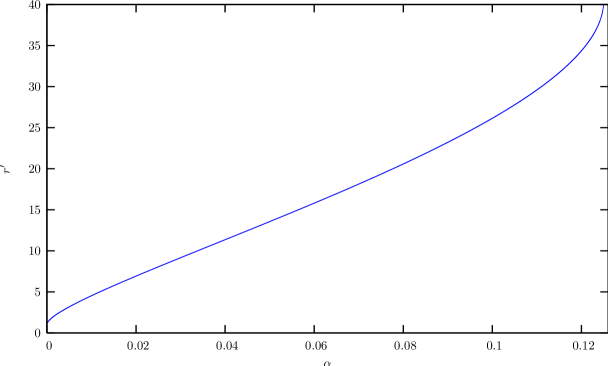
Figure 1: The figure shows a plot of the radius of the disc $r^{\prime}$ measured in arbitrary units, as a function of the parameter $\alpha$. In the non–relativistic case, for which $\alpha=0$, the radius of the disc is exactly the same as the one predicted by Ulrich (1976). For the extreme hyperbolic model, when $\alpha\rightarrow 1/8$, the radius of the disc grows without limit.

The fact that the disc radius grows monotonically as $\alpha$ approaches the value $1/8$ means that the density of the disc should be distributed in a more homogeneous way. Figure 2 shows density profiles evaluated in the equatorial plane $\theta=\pi/2$ as a function of the distance to the central object. In all cases the particle number density diverges in the origin because it represents a point of accumulated material. The case $\alpha=0$ corresponds to the non–relativistic Ulrich model and apart from the divergence that the particle number density has at $r=0$ it also grows without limit at the radius of the disc $r_{\text{dN}}$. This is generally attributed to border effects that appear because the disc has been assumed to be thin (see e.g. Mendoza et al., 2004, and references therein). However, as Figure 2 shows, the divergence of the particle number density at the border of the disc disappears as soon as $\alpha$ moves away from a null value. Furthermore, it does so in such a way that the density of the disc varies very smoothly throughout the disc as $\alpha\rightarrow 1/8$.

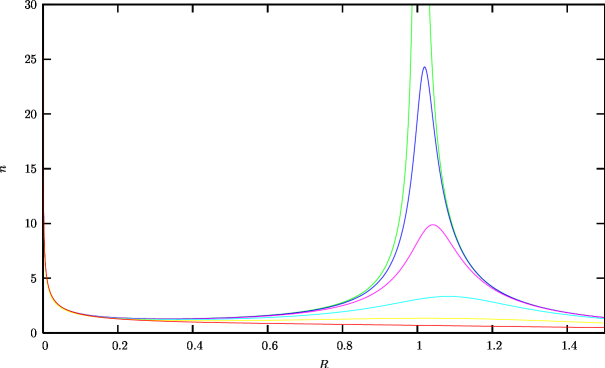
Figure 2: The plots represent different particle number densities $n$ measured in units of $n_{0}$, as a function of the radial distance $R$ (measured in units of $r_{*}$) evaluated in the equator, i.e. for which the polar angle $\theta=\pi/2$. From bottom to top the models correspond to values $\alpha$ of $1/8,\ 10^{-1},\ 10^{-2},\ 10^{-3},\ 10^{-4}$ and $10^{-5}$. All profiles diverge at the origin because of accumulated material at that point. The particle number density diverges in the Newtonian limit (for which $\alpha\rightarrow 0$) at the border of the disc, which corresponds for that particular case to $R\rightarrow 1$ (Mendoza et al., 2004). However, this singularity disappears and softens the density profile in the disc as $\alpha\rightarrow 1/8$.

The results of section 5 can be used to compare with the pseudo–Newtonian Paczynsky & Wiita (1980) approximation used by Lee & Ramirez-Ruiz (2006). Figure 3 shows a comparison between the full relativistic solution with the pseudo–Newtonian approximation. It is clear from the images that the solution differs not only at small radii, near the Schwarzschild radius, but also at large scales. This is due to the strength of the gravitational field produced by the central source, which makes particles approach the equator quite rapidly. For instance, near the event horizon there are fluid particles that appear to be swallowed by the hole when described by a pseudo–Newtonian potential. However, the complete relativistic solution shows that for this particular case some of those particles are not swallowed directly by the hole, but are injected to the accretion disc.

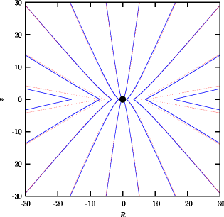
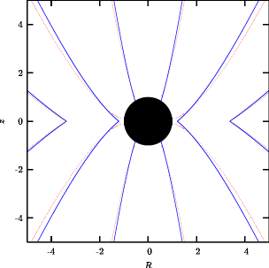
Figure 3: The figure shows a comparison between the fully relativistic solution presented in this article (continuous lines) with the Newtonian Paczynsky & Wiita (1980) numerical approximations made by Lee & Ramirez-Ruiz (2006) (dotted lines). Distances in the plot are measured in units of the Schwarzschild radius. The plot is a projection at an azimuthal angle $\varphi=\text{const}$. The length $R$ is the radial distance measured in the equator. In both cases, the streamlines were calculated in the extreme hyperbolic case for which $\alpha=1/8$, i.e. the specific angular momentum for a particular fluid particle is twice the Schwarzschild radius. Particles were considered to be uniformly rotating at a distance of $50$ Schwarzschild radius measured from the origin. Both, the small and large scale panels show that the complete relativistic solution differs significantly from their calculations. The pseudo–Newtonian Paczynsky & Wiita approximations were kindly provided by W. H. Lee.

The work presented in this article represents a general relativistic approach to the Newtonian accretion flow first proposed by Ulrich (1976). The main features of the accretion flow are still valid with the important consequence that, the radius of the equatorial accretion disc grows from its Newtonian value for the Ulrich case up to infinity in the extreme hyperbolic situation, for which the angular momentum is twice the Schwarzschild radius. As a consequence, the particle number density diverges on the border of the disc only for the Newtonian case described by Ulrich. This is due to the fact that, when the radius of the disc grows, the particle number density on it rearranges in such a way that it smoothly softens as the extreme hyperbolic case is approached. Figures 4 and 5 show streamlines and density isocontours for different values of the parameter $\alpha$.

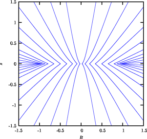
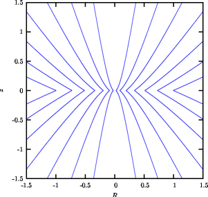
Figure 4: Streamlines for values of the parameter $\alpha=10^{-5},\ 0.12$ from left to right are shown in the figure. Lengths are measured in units of the radius $r_{*}$. The equatorial radius is labelled by $R$. The case $\alpha=10^{-5}$ is very close to the Newtonian one (see for example Mendoza et al. (2004)). This particular case shows that the streamlines are accumulated at $R=1$, which corresponds to the Newtonian radius $r_{\text{dN}}$. However, the right panel shows that as $\alpha$ approaches the value $1/8$ the streamlines are not packed together any longer.

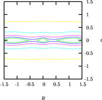
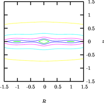
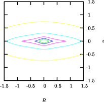
Figure 5: Particle number density isocontours for $\alpha=10^{-5},\ 0.05,\ 0.12$ are shown in each diagram. The left panel roughly corresponds to the non–relativistic case as described by Mendoza et al. (2004). All models show a density divergence at the origin. However, only the Newtonian case exhibits another divergence at the border of the disc $R=1$. Lengths in the plot are measured in units of the radius $r_{*}$ and the density isocontours correspond to values of $n/n_{0}=0.1,\ 0.6,\ 1.1,\ 1.6,\ 2.1,\ 2.6$.

7 Acknowledgements

We dedicate the present article to the vivid memory of Sir Hermann Bondi who pioneered the studies of spherical accretion. We would like to thank William Lee for providing his numerical Paczynsky & Wiita pseudo–Newtonian results in order to make comparisons with the exact analytic solution presented in this article. The authors gratefully acknowledge financial support from DGAPA–UNAM (IN119203).

References

- Beloborodov & Illarionov (2001) Beloborodov, A. M., & Illarionov, A. F. 2001, MNRAS, 323, 167
- Birkhoff (1923) Birkhoff, G. 1923, Relativity and Modern Physics (Harvard University Press, Cambridge, MA)
- Bondi (1952) Bondi, H. 1952, MNRAS, 112, 195
- Bondi (2005) —. 2005, Accretion (The Scientific Legacy of Fred Hoyle), 55–57
- Cassen & Moosman (1981) Cassen, P., & Moosman, A. 1981, Icarus, 48, 353
- Cayley (1961) Cayley, A. 1961, An elementary treatise on elliptic functions (New York : Dover, 1961)
- Chandrasekhar (1983) Chandrasekhar, S. 1983, The Mathematical Theory of Black Holes (Oxford University)
- Frank et al. (2002) Frank, J., King, A., & Raine, D. J. 2002, Accretion Power in Astrophysics: Third Edition (Accretion Power in Astrophysics, by Juhan Frank and Andrew King and Derek Raine, pp. 398. ISBN 0521620538. Cambridge, UK: Cambridge University Press, February 2002.)
- Hancock (1917) Hancock, H. 1917, Elliptic Integrals (New York : Dover, 1917)
- Landau & Lifshitz (1994a) Landau, L., & Lifshitz, E. 1994a, Course of Theoretical Physics, Vol. 2, The Classical Theory of Fields, 4th edn. (Pergamon)
- Landau & Lifshitz (1994b) —. 1994b, Course of Theoretical Physics, Vol. 1, Mechanics, 4th edn. (Pergamon)
- Lawden (1989) Lawden, D. 1989, Elliptic Functions and Applications (Springer)
- Lee & Ramirez-Ruiz (2006) Lee, W. H., & Ramirez-Ruiz, E. 2006, ApJ, 641, 961
- Mendoza et al. (2004) Mendoza, S., Cantó, J., & Raga, A. C. 2004, Revista Mexicana de Astronomia y Astrofisica, 40, 147
- Michel (1972) Michel, F. C. 1972, Ap&SS, 15, 153
- Misner et al. (1973) Misner, C. W., Thorne, K. S., & Wheeler, J. A. 1973, Gravitation (San Francisco: W.H. Freeman and Co., 1973)
- Novikov & Frolov (1990) Novikov, I., & Frolov, V. 1990, Black hole physics (CUP)
- Paczynsky & Wiita (1980) Paczynsky, B., & Wiita, P. J. 1980, A&A, 88, 23
- Stanyukovich (1960) Stanyukovich, K. P. 1960, Non-steady motion of continuous media (Oxford University Press, Oxford, U.K.)
- Ulrich (1976) Ulrich, R. K. 1976, ApJ, 210, 377
- Wald (1984) Wald, R. 1984, General Relativity (University of Chicago)