Gravitational Radiation from Two-Body Systems 

Abstract

Thanks to the new generation of gravitational wave detectors LIGO and VIRGO, the theory of general relativity will face new and important confrontations to observational data with unprecedented precision. Indeed the detection and analysis of the gravitational waves from compact binary star systems requires beforehand a very precise solution of the two-body problem within general relativity. The approximation currently used to solve this problem is the post-Newtonian one, and must be pushed to high order in order to describe with sufficient accuracy (given the sensitivity of the detectors) the inspiral phase of compact bodies, which immediately precedes their final merger. The resulting post-Newtonian “templates” are currently known to 3.5PN order, and are used for searching and deciphering the gravitational wave signals in VIRGO and LIGO.

1 Introduction

A compelling motivation for accurate computations of the gravitational radiation field generated by compact binary systems (i.e., made of neutron stars and/or black holes) is the need for accurate templates to be used in the data analysis of the current and future generations of laser interferometric gravitational wave detectors. It is indeed recognized that the inspiral phase of the coalescence of two compact objects represents an extremely important source for the ground-based detectors such as LIGO and VIRGO, provided that their total mass does not exceed say 10 or 20 $M_{\odot}$ (this includes the very interesting case of double neutron-star systems), and for space-based detectors like LISA, in the case of the coalescence of two galactic black holes, if the masses are within the range between say $10^{5}$ and $10^{8}\,M_{\odot}$.

For these sources the post-Newtonian (PN) approximation scheme has proved to be the appropriate theoretical tool in order to construct the necessary templates. A program started long ago with the goal of obtaining these templates with 3PN and even 3.5PN accuracy.  Several studies, e.g. [1, 2], have shown that such a high PN precision is probably sufficient, not only for detecting the signals in LIGO/VIRGO, but also for analyzing them and accurately measuring the parameters of the binary (such high-accuracy templates will also be of great value for detecting massive black-hole mergers in LISA). The templates have been first completed through 2PN order [3]. The 3.5PN accuracy (in the case where the compact objects have negligible intrinsic spins) has been achieved more recently [4, 5].

The calculation of the 3PN order turned out to be very intricate and quite subtle. The first step has been to compute all the terms, in both the 3PN equations of motion [6, 7, 8, 9, 10] and 3.5PN gravitational radiation field [11, 12, 13], by means of the Hadamard self-field regularization [14, 15]. A regularization is needed in this problem in order to remove the infinite self-field of point masses. However, a few terms were left undetermined by Hadamard’s regularization, which correspond to some incompleteness of this regularization occurring at the 3PN order. These terms could be parametrized by some unknown numerical coefficients called ambiguity parameters. The second step has been to use the more powerful dimensional regularization [16], which is technically based on analytic continuation in the dimension of space, which finally enabled to fix the values of all the ambiguity parameters [17, 18, 5, 19].

In Section 2 of this article we review and comment on the striking appearance of Hadamard self-field regularization parameters at 3PN order, and on their computation using dimensional regularization. Section 3 is devoted to the notion of the multipole moments of an isolated post-Newtonian extended source, at the basis of the construction of gravitational-wave post-Newtonian templates. In Section 4 we present two checks of the values of the latter ambiguity parameters, coming from the comparison between the binary’s dipole moment and its center-of-mass vector on the one hand, and based on an argument from classical field-theory diagrams on the other hand. Finally, in Section 5, we consider the limiting case where one of the masses is exactly zero, and the remaining one moves with uniform velocity, and show that such “boosted Schwarzschild solution” limit yields the determination of the third ambiguity parameter in the radiation field. These tests, altogether, provide a verification, independent of dimensional regularization, for all the ambiguity parameters in the 3PN gravitational radiation field.

2 Hadamard regularization parameters

The standard Hadamard regularization yields some ambiguous results for the computation of certain integrals at the 3PN order, as Jaranowski and Schäfer [6, 7] first noticed in their computation of the equations of motion of point particles within the ADM-Hamiltonian formulation of general relativity. Hadamard’s regularization is based on the notion of partie finie of a singular function, given by the angular integral of the finite part coefficient in the singular expansion of that function near a singular point, and the related notion of partie finie of a divergent integral. It was shown [6, 7] that there are two and only two types of ambiguous terms in the 3PN Hamiltonian, which were then parametrized by two unknown numerical coefficients $\omega_{\mathrm{static}}$ and $\omega_{\mathrm{kinetic}}$.

Motivated by the previous result, Blanchet and Faye introduced an extended version of Hadamard’s regularization [20, 21], which is mathematically well-defined and free of ambiguities; in particular it yields unique results for the computation of any of the integrals occuring in the 3PN equations of motion. Unfortunately, the extended Hadamard regularization turned out to be in a sense incomplete, because it was found [8, 9] that the 3PN equations of motion involve one and only one unknown numerical constant, called $\lambda$, which cannot be determined within the method. The comparison with the work [6, 7], on the basis of the computation of the invariant energy of compact binaries moving on circular orbits, revealed [8] that

$$\omega_{\mathrm{kinetic}} = \frac{41}{24}\,,$$ (1)

$$\omega_{\mathrm{static}} = -\frac{11}{3}\lambda-\frac{1987}{840}\,.$$ (2)

Therefore, the ambiguity $\omega_{\mathrm{kinetic}}$ is fixed, while $\lambda$ is equivalent to the other ambiguity $\omega_{\mathrm{static}}$. Notice that the value (1) for the kinetic ambiguity parameter $\omega_{\mathrm{kinetic}}$, which is in factor of some velocity dependent terms, is the only one for which the 3PN equations of motion are Poincaré invariant. Fixing up this value was possible because the extended Hadamard regularization [20, 21] was defined in such a way that it keeps the Poincaré invariance.

The appearance of one and only one physical unknown coefficient $\lambda$ in the equations of motion constitutes a quite striking fact, that is related specifically with the use of some Hadamard-type regularization. Technically speaking, the presence of the parameter $\lambda$ is associated with the so-called “non-distributivity” of Hadamard’s regularization.  Mathematically speaking, $\lambda$ is probably related to the fact that it is impossible to construct a distributional derivative operator satisfying the Leibniz rule for the derivation of the product. The Einstein field equations can be written into many different forms, by shifting the derivatives and operating some terms by parts with the help of the Leibniz rule. All these forms are equivalent in the case of regular sources, but since the distributional derivative operator violates the Leibniz rule they become inequivalent for point particles. Finally, physically speaking, we can argue that $\lambda$ has its root in the fact that, in a complete computation of the equations of motion valid for two regular extended weakly self-gravitating bodies, many non-linear integrals, when taken individually, start depending, from the 3PN order, on the internal structure of the bodies, even in the “compact-body” limit where the radii tend to zero. However, when considering the full equations of motion, we expect that all the terms depending on the internal structure can be removed, in the compact-body limit, by a coordinate transformation (or by some appropriate shifts of the central world lines of the bodies), and that finally $\lambda$ is given by a pure number, for instance a rational fraction, independent of the details of the internal structure of the compact bodies. From this argument (which could be justified by invoking the effacing principle in general relativity [22]) the value of $\lambda$ is necessarily the one we shall obtain below, Eq. (4), and will be valid for any compact objects, for instance black holes.

The ambiguity parameter $\omega_{\mathrm{static}}$, which is in factor of some static, velocity-independent term, was computed by Damour, Jaranowski and Schäfer [17] by means of dimensional regularization, instead of some Hadamard-type one, within the ADM-Hamiltonian formalism. Their result is

$$\omega_{\mathrm{static}}=0\,.$$ (3)

As Damour et al. [17] argue, clearing up the static ambiguity is made possible by the fact that dimensional regularization, contrary to Hadamard’s regularization, respects all the basic properties of the algebraic and differential calculus of ordinary functions: associativity, commutativity and distributivity of point-wise addition and multiplication, Leibniz’s rule, and the Schwarz lemma. In this respect, dimensional regularization is certainly better than Hadamard’s one, which does not respect the distributivity of the product and unavoidably violates at some stage the Leibniz rule for the differentiation of a product.

The ambiguity parameter $\lambda$ is fixed from the result (3) and the necessary link (2) provided by the equivalence between the harmonic-coordinates and ADM-Hamiltonian formalisms. However, $\lambda$ was also computed directly by Blanchet, Damour and Esposito-Farèse [18] applying dimensional regularization to the 3PN equations of motion in harmonic coordinates (in the line of Refs. [8, 9]). The end result,

$$\lambda=-\frac{1987}{3080}\,,$$ (4)

is in full agreement with Eq. (3). Besides the independent confirmation of the value of $\omega_{\mathrm{static}}$ or $\lambda$, the work [18] provides also a confirmation of the consistency of dimensional regularization, because the explicit calculations are entirely different from the ones of Ref. [17]: harmonic coordinates are used instead of ADM-type ones, the work is at the level of the equations of motion instead of the Hamiltonian, a different form of Einstein’s field equations is solved by a different iteration scheme.

Let us comment here that the use of a self-field regularization, be it dimensional or based on Hadamard’s partie finie, signals a somewhat unsatisfactory situation on the physical point of view, because, ideally, we would like to perform a complete calculation valid for extended bodies, taking into account the details of the internal structure of the bodies (energy density, pressure, internal velocity field). By considering the limit where the radii of the objects tend to zero, one should recover the same result as obtained by means of the point-mass regularization. This would demonstrate the suitability of the regularization. This program was undertaken at the 2PN order by Grishchuk and Kopeikin [23, 24] who derived the equations of motion of two extended fluid balls, and obtained equations of motion depending only on the two masses $m_{1}$ and $m_{2}$ of the compact bodies. At the 3PN order we expect that the extended-body program should give the value of the regularization parameter $\lambda$ (maybe after some gauge transformation to remove the terms depending on the internal structure). Ideally, its value should be confirmed by independent and more physical methods. One such method is the one of Itoh and Futamase [25, 26], who derived the 3PN equations of motion in harmonic coordinates by means of a particular variant of the famous “surface-integral” method introduced long ago by Einstein, Infeld and Hoffmann [27]. This approach is interesting because it is based on the physical notion of extended compact bodies in general relativity, and is free of the problems of ambiguities due to Hadamard’s self-field regularization. The end result of Refs. [25, 26] is in agreement with the complete 3PN equations of motion in harmonic coordinates [8, 9] and, moreover, is unambiguous, as it does determine the ambiguity parameter $\lambda$ to exactly the value (4).

We next consider the problem of the binary’s radiation field, where the same phenomenon occurs, with the appearance of some Hadamard regularization ambiguity parameters at 3PN order. More precisely, Blanchet, Iyer and Joguet [12], in their computation of the 3PN compact binary’s mass quadrupole moment $\mathrm{I}_{ij}$, found it necessary to introduce three Hadamard regularization constants $\xi$, $\kappa$ and $\zeta$, which are additional to (and independent of) the equation-of-motion related constant $\lambda$. The total gravitational-wave flux at 3PN order, in the case of circular orbits, was found to depend on a single combination of the latter constants, $\theta=\xi+2\kappa+\zeta$, and the binary’s orbital phase, for circular orbits, involves only the linear combination of $\theta$ and $\lambda$ given by $\hat{\theta}=\theta-7\lambda/3$, as shown in [4].

Dimensional regularization (instead of Hadamard’s) was applied in Refs. [5, 19] to the computation of the 3PN radiation field of compact binaries, finally leading to the following unique values for the ambiguity parameters

$$\xi = -\frac{9871}{9240}\,,$$ (5)

$$\kappa = 0\,,$$ (6)

$$\zeta = -\frac{7}{33}\,.$$ (7)

These values represent the end result of dimensional regularization. However, we shall review in the present Article some alternative calculations which provide some checks, independent of dimensional regularization, for all the parameters (5)–(7).

The result (5)–(7) completes the problem of the general relativistic prediction for the templates of inspiralling compact binaries up to 3PN order (and actually up to 3.5PN order as the corresponding tail terms have already been determined [11]). The relevant combination of the parameters entering the 3PN energy flux in the case of circular orbits is now fixed to be

$$\theta\equiv\xi+2\kappa+\zeta=-\frac{11831}{9240}\,.$$ (8)

The orbital phase of compact binaries, in the adiabatic inspiral regime (i.e., evolving by radiation reaction), involves at 3PN order a combination of parameters which is determined as

$$\hat{\theta}\equiv\theta-\frac{7}{3}\lambda=\frac{1039}{4620}\,.$$ (9)

The fact that the numerical value of this parameter is quite small, $\hat{\theta}\simeq 0.22489$, indicates that the 3PN (or, even better, 3.5PN) order should provide an excellent approximation for both the on-line search and the subsequent off-line analysis of gravitational wave signals from inspiralling compact binaries in the LIGO and VIRGO detectors.

3 The multipolar post-Newtonian formalism

3.1 Multipole moments of a post-Newtonian extended source

The multipole moments of a post-Newtonian (PN) source, by which we mean a source which is at once slowly moving, weakly stressed and weakly self-gravitating, are crucial for the present gravitational wave generation formalism. They are obtained in Ref. [28] as functionals of the PN expansion of the pseudo-stress energy tensor $\tau^{\mu\nu}$ of the matter and gravitational fields in the harmonic coordinate system. The pseudo-tensor $\tau^{\mu\nu}$ has a non-compact support because of the contribution of the gravitational field which extends up to infinity from the source. Let us denote the formal PN expansion of the pseudo tensor by means of an overbar, so that $\overline{\tau}^{\mu\nu}=\mathrm{PN}[\tau^{\mu\nu}]$. The two types of multipole moments of the gravitating source, mass-type $\mathrm{I}_{L}$ moments and current-type ones $\mathrm{J}_{L}$, are then given by 

$$\mathrm{I}_{L}(t) = \frac{1}{c^{2}}\,\mathop{\mathrm{FP}}_{B=0}\int d^{3}\mathbf{x}\,r^{B}\left\{\hat{x}_{L}\,\Bigl{(}\mathop{\overline{\tau}}_{[\ell]}{}^{\!\!00}+\mathop{\overline{\tau}}_{[\ell]}{}^{\!\!ii}\Bigr{)}\right.$$ (10)

$$\qquad\qquad\left.-\frac{4(2\ell+1)}{c(\ell+1)(2\ell+3)}\,\hat{x}_{iL}\,\mathop{\dot{\overline{\tau}}}_{[\ell+1]}{}^{\!\!\!\!i0}\right.$$

$$\qquad\qquad\left.+\frac{2(2\ell+1)}{c^{2}(\ell+1)(\ell+2)(2\ell+5)}\,\hat{x}_{ijL}\,\mathop{\ddot{\overline{\tau}}}_{[\ell+2]}{}^{\!\!\!\!ij}\right\}\,,$$

$$\mathrm{J}_{L}(t) = \frac{1}{c}\,\mathop{\mathrm{FP}}_{B=0}\varepsilon_{ab\langle i_{\ell}}\int d^{3}\mathbf{x}\,r^{B}\left\{\hat{x}_{L-1\rangle a}\mathop{\overline{\tau}}_{[\ell]}{}^{\!\!b0}\right.$$ (11)

$$\qquad\qquad\left.-\frac{2\ell+1}{c(\ell+2)(2\ell+3)}\,\hat{x}_{L-1\rangle ac}\mathop{\dot{\overline{\tau}}}_{[\ell+1]}{}^{\!\!\!\!bc}\right\}\,.$$

Since Eqs. (10)–(11) are valid only in the sense of PN expansions, the operational meaning of the underscript $[\ell]$ in (10)–(11) is actually that of an infinite PN series, which is given by

$$\mathop{\overline{\tau}}_{[\ell]}{}^{\!\!\mu\nu}(\mathbf{x},t) = \sum_{k=0}^{+\infty}\,\alpha_{k,\ell}\,\left(\frac{r}{c}\frac{\partial}{\partial t}\right)^{2k}\overline{\tau}^{\mu\nu}(\mathbf{x},t)\,,$$ (12)

$$\alpha_{k,\ell} = \frac{(2\ell+1)!!}{(2k)!!(2\ell+2k+1)!!}\,.$$ (13)

A basic feature of the expressions of the moments is that the integral formally extends over the whole support of the PN expansion of the stress-energy pseudo-tensor, $\overline{\tau}^{\mu\nu}$, i.e. from $r\equiv|\mathbf{x}|=0$ up to infinity. Recall that a formal PN series such as $\overline{\tau}^{\mu\nu}$ is physically meaningful only within the near-zone. Therefore the integrals (10)–(11) physically refer to a result obtained from near-zone quantities only (in the formal limit where $c\rightarrow+\infty$). However, it was found extremely useful in Ref. [28] to mathematically extend the integrals up to $r\rightarrow+\infty$. This was made possible by the use of the prefactor $r^{B}$, together with a process of analytic continuation in the complex $B$ plane.  This shows up in Eqs. (10)–(11) as the crucial Finite Part (FP) operation, when $B\rightarrow 0$, which technically allows one to uniquely define integrals which would otherwise be divergent at their upper boundary, $r=|\mathbf{x}|\rightarrow+\infty$. See Ref. [28] for the proof and details.

3.2 Surface-integral expressions of the multipole moments

Let us next review the recent derivation [29] of an alternative form of the PN source moments (10)–(11) in terms of two-dimensional surface integrals. Such a possibility of expressing the moments, for general $\ell$ and at any PN order, as some surface integrals is quite useful for practical purposes, as we shall show in the application we consider in Section 5. In keeping with the fact that the “volume integrals” Eqs. (10)–(11) physically involve only near-zone quantities, the “surface integrals” into which we shall transform the moments $\mathrm{I}_{L}$ and $\mathrm{J}_{L}$ physically refer to an operation which extracts some coefficients in the “far near-zone” expansion of the gravitational field, i.e. in the expansion in increasing powers of $1/r$ of the PN-expanded near-zone metric. Technically, as our starting point (10)–(11) is made of integrals extended up to $r\rightarrow+\infty$, our mathematical manipulations below will involve “surface terms” on arbitrary large spheres $r=\mathcal{R}$. All these manipulations will be mathematically well-defined because of the properties of complex analytic continuation in $B$.

The basic idea is to go from the “source term”, $\overline{\tau}^{\mu\nu}$, to the corresponding “solution” $\overline{h}^{\mu\nu}$, via integrating by parts the Laplace operator present in the Einstein field equation in harmonic coordinates, namely $\overline{\tau}^{\mu\nu}=\frac{c^{4}}{16\pi G}\,\square\,\overline{h}^{\mu\nu}$, where $\overline{h}^{\mu\nu}$ is the (PN expansion of the) basic gravitational field variable, satisfying the harmonic-coordinate condition $\partial_{\nu}\overline{h}^{\mu\nu}=0$. From Eq. (12) we have

$$\int d^{3}\mathbf{x}\,r^{B}\,\hat{x}_{L}\,\mathop{\overline{\tau}}_{[\ell]}{}^{\!\!\mu\nu}=\frac{c^{4}}{16\pi G}\sum_{k=0}^{+\infty}\,\alpha_{k,\ell}\,\left(\frac{d}{cdt}\right)^{\!2k}\int d^{3}\mathbf{x}\,r^{B+2k}\,\hat{x}_{L}\,\Box\,\overline{h}^{\mu\nu}\,,$$ (14)

in the right-hand-side of which we insert $\Box=\Delta-\left(\frac{\partial}{c\,\partial t}\right)^{2}$, and operate the Laplacian by parts using $\Delta(r^{B+2k}\,\hat{x}_{L})=(B+2k)(B+2\ell+2k+1)r^{B+2k-2}\,\hat{x}_{L}$. In the process we can ignore the all-integrated surface terms because they are identically zero by complex analytic continuation, from the case where the real part of $B$ is chosen to be a large enough negative number. Using the expression of the coefficients (13), we are next led to the alternative expression

$$\int d^{3}\mathbf{x}\,r^{B}\,\hat{x}_{L}\,\mathop{\overline{\tau}}_{[\ell]}{}^{\!\!\mu\nu}=\frac{c^{4}}{16\pi G}\sum_{k=0}^{+\infty}\,B(B+2\ell+4k+1)\,\alpha_{k,\ell}\left(\frac{d}{cdt}\right)^{\!2k}\!\!\int d^{3}\mathbf{x}\,r^{B+2k-2}\,\hat{x}_{L}\,\overline{h}^{\mu\nu}\,.$$ (15)

A remarkable feature of this result, which is the basis of our new expressions, is the presence of an explicit factor $B$ in front of the integral. The factor means that the result depends only on the occurrence of poles, $\propto 1/B^{p}$, in the boundary of the integral at infinity: $r\rightarrow+\infty$ with $t=\mathrm{const}$.

Thanks to the factor $B$ we can replace the integration domain of Eq. (15) by some outer domain of the type $r>\mathcal{R}$, where $\mathcal{R}$ denotes some large arbitrary constant radius. The integral over the inner domain $r<\mathcal{R}$ is always zero in the limit $B\rightarrow 0$ because the integrand is constructed from $\overline{\tau}^{\mu\nu}$, and we are considering extended regular PN sources, without singularities. Now, in the outer (but still near-zone) domain we can replace the PN metric coefficients $\overline{h}^{\mu\nu}$ by the expansion in increasing powers of $1/r$ of the PN-expanded metric, which is identical to the multipolar expansion of the PN-expanded metric, that we shall denote by $\mathcal{M}\bigl{(}\overline{h}^{\mu\nu}\bigr{)}$. Hence we have

$$\int d^{3}\mathbf{x}\,r^{B}\,\hat{x}_{L}\mathop{\overline{\tau}}_{[\ell]}{}^{\!\!\mu\nu}=\frac{c^{4}}{16\pi G}\sum_{k=0}^{+\infty}B(B+2\ell+4k+1)\,\alpha_{k,\ell}\left(\frac{d}{cdt}\right)^{\!2k}\!\!\!\int_{r>\mathcal{R}}\!\!d^{3}\mathbf{x}\,r^{B+2k-2}\hat{x}_{L}\mathcal{M}\bigl{(}\overline{h}^{\mu\nu}\bigr{)}\,.$$ (16)

We want now to make use of a more explicit form of the far near-zone expansion $\mathcal{M}\bigl{(}\overline{h}^{\mu\nu}\bigr{)}$, whose general structure is known. It consists of terms proportional to arbitrary powers of $1/r$, and multiplied by powers of the logarithm of $r$; more precisely,

$$\mathcal{M}\bigl{(}\overline{h}^{\mu\nu}\bigr{)}(\mathbf{x},t)=\sum_{a,\,b}\frac{(\ln r)^{b}}{r^{a}}\,\varphi_{a,b}^{\mu\nu}(\mathbf{n},t)\,,$$ (17)

where $a$ can take any positive or negative integer values, and $b$ can be any positive integer: $a\in\mathbb{Z}$, $b\in\mathbb{N}$. The coefficients $\varphi_{a,b}^{\mu\nu}$ depend on the unit direction $\mathbf{n}\equiv\mathbf{x}/r$ and on the coordinate time $t$ (in the harmonic coordinate system). The structure (17) for the multipolar expansion of the near-zone (PN-expanded) metric is a consequence of the so-called matching equation

$$\mathcal{M}\bigl{(}\overline{h}^{\mu\nu}\bigr{)}\equiv\overline{\mathcal{M}\left(h^{\mu\nu}\right)}\,,$$ (18)

which says that the multipolar re-expansion of the PN metric $\overline{h}^{\mu\nu}$ agrees, in the sense of formal series, with the near-zone re-expansion (also denoted with an overbar) of the external multipolar metric $\mathcal{M}\left(h^{\mu\nu}\right)$ (see [28] for details). Inserting Eq. (17) into (16), we are therefore led to the computation of the integral

$$\int_{r>\mathcal{R}}\!\!d^{3}\mathbf{x}\,r^{B+2k-2}\,\hat{x}_{L}\,\mathcal{M}\bigl{(}\overline{h}^{\mu\nu}\bigr{)}=\sum_{a,\,b}\int_{\mathcal{R}}^{+\infty}dr\,r^{B+2k+\ell-a}\,(\ln r)^{b}\int d\Omega\,\hat{n}_{L}\,\varphi_{a,b}^{\mu\nu}(\mathbf{n},t)\,,$$ (19)

where $d\Omega$ is the solid angle element associated with the unit direction $\mathbf{n}$ (and $\hat{n}_{L}\equiv\hat{x}_{L}/r^{\ell}$). The radial integral can be trivially integrated by analytic continuation in $B$, with result

$$\int_{\mathcal{R}}^{+\infty}dr\,r^{B+2k+\ell-a}\,(\ln r)^{b}=-\left(\frac{d}{dB}\right)^{b}\left[\frac{\mathcal{R}^{B+2k+\ell-a+1}}{B+2k+\ell-a+1}\right]\,.$$ (20)

Remember that we are ultimately interested only in the analytic continuation of such integrals down to $B=0$. And as an integral such as (20) is multiplied by a coefficient which is proportional to $B$, we must control the poles of Eq. (20) at $B=0$. Those poles are in general multiple because of the presence of powers of $\ln r$ in the expansion, and the consecutive multiple differentiation with respect to $B$ shown in Eq. (20). The poles at $B=0$ clearly come from a single value of $a$, namely $a=2k+\ell+1$. For that value, the “multiplicity” of the pole takes the value $b+1$. Here a useful simplification comes from the fact that the factor in front of the integrals in (16) is of the form $\sim B(B+K)$. In other words, this factor contains only the first and second powers of $B$. Therefore, only the simple and double poles $1/B$ and $1/B^{2}$ in (20) can contribute to the final result. Hence, we conclude that it is enough to consider the values $b=0,1$ for the exponent $b$ of $\ln r$ in the expansion (17).

To express the result in the most convenient manner let us introduce a special notation for some relevant combination of coefficients $\varphi_{a,b}^{\mu\nu}(\mathbf{n},t)$, which as we just said correspond exclusively to the values $a=\ell+2k+1$ and $b=0$ or $1$. Namely,

$$\Psi_{k,\ell}^{\mu\nu}(\mathbf{n},t)\equiv\alpha_{k,\ell}\Bigl{[}-(2\ell+4k+1)\varphi_{2k+\ell+1,0}^{\mu\nu}(\mathbf{n},t)+\varphi_{2k+\ell+1,1}^{\mu\nu}(\mathbf{n},t)\Bigr{]}\,,$$ (21)

in which we have absorbed the numerical coefficient $\alpha_{k,\ell}$ defined by (13). With this notation we then obtain

$$\mathop{\mathrm{FP}}_{B=0}\,B\,(B+2\ell+4k+1)\,\alpha_{k,\ell}\int_{r>\mathcal{R}}\!\!d^{3}\mathbf{x}\,r^{B+2k-2}\,\hat{x}_{L}\,\mathcal{M}\bigl{(}\overline{h}^{\mu\nu}\bigr{)}=4\pi\left\langle\,\hat{n}_{L}\,\Psi_{k,\ell}^{\mu\nu}\right\rangle\,,$$ (22)

where the brackets refer to the spherical or angular average (at coordinate time $t$), i.e.

$$\left\langle\,\hat{n}_{L}\,\Psi_{k,\ell}^{\mu\nu}\right\rangle(t)\equiv\int\frac{d\Omega}{4\pi}\,\hat{n}_{L}\,\Psi_{k,\ell}^{\mu\nu}(\mathbf{n},t)\,.$$ (23)

The quantities (23) are integrals over a unit sphere, and can rightly be referred to as surface integrals. These surface integrals are the basic blocks entering our alternative expressions for the multipole moments. If we wish to physically think of them as integrals over some two-surface surrounding the source, we can roughly consider that this two-surface is located at a radius $\mathcal{R}$, with $a\ll\mathcal{R}\ll c\,T$. Anyway, the important point is that, as we can see from Eq. (23), the surface integrals, and therefore the multipole moments, are strictly independent of the choice of the intermediate scale $\mathcal{R}$ which entered our reasoning.

Finally, we are in a position to write down the following final results for an alternative form of the source multipole moments (10)–(11), expressed solely in terms of the surface integrals of the type (23),

$$\mathrm{I}_{L} = \frac{c^{2}}{4\,G}\,\sum_{k=0}^{+\infty}\biggl{\{}\left(\frac{d}{cdt}\right)^{\!\!2k}\left\langle\,\hat{n}_{L}\left(\Psi_{k,\ell}^{00}+\Psi_{k,\ell}^{ii}\right)\right\rangle$$ (24)

$$\qquad\qquad-\frac{4(2\ell+1)}{(\ell+1)(2\ell+3)}\,\left(\frac{d}{cdt}\right)^{\!\!2k+1}\left\langle\,\hat{n}_{iL}\,\Psi_{k,\ell+1}^{i0}\right\rangle$$

$$\qquad\qquad+\frac{2(2\ell+1)}{(\ell+1)(\ell+2)(2\ell+5)}\,\left(\frac{d}{cdt}\right)^{\!\!2k+2}\left\langle\,\hat{n}_{ijL}\,\Psi_{k,\ell+2}^{ij}\right\rangle\biggr{\}}\,,$$

$$\mathrm{J}_{L} = \frac{c^{3}}{4\,G}\,\varepsilon_{ab\langle i_{\ell}}\sum_{k=0}^{+\infty}\biggl{\{}\left(\frac{d}{cdt}\right)^{\!\!2k}\left\langle\,\hat{n}_{L-1\rangle a}\,\Psi_{k,\ell}^{b0}\right\rangle$$ (25)

$$\qquad\qquad-\frac{2\ell+1}{(\ell+2)(2\ell+3)}\,\left(\frac{d}{cdt}\right)^{\!\!2k+1}\left\langle\,\hat{n}_{L-1\rangle ac}\,\Psi_{k,\ell+1}^{bc}\right\rangle\biggr{\}}\,.$$

4 Multipole moments of two-body systems

4.1 Quadrupole and dipole moments, and the center-of-mass vector

Let us show how a particular combination of ambiguity parameters can be determined within Hadamard’s regularization and confirm the result of dimensional regularization. For this purpose we use the computations in Ref. [13] of the mass-type quadrupole $\mathrm{I}_{ij}$ and dipole $\mathrm{I}_{i}$ moments of point particle binaries at the 3PN order. These were derived by applying the expression (10) [with $\ell=1,2$] to a binary systems of point masses, following the rules of the Hadamard regularization, in the so-called “pure Hadamard-Schwartz” (pHS) variant of it. Following the definition of Ref. [18], the pHS regularization is a specific, minimal Hadamard-type regularization of integrals, based on the usual Hadamard partie finie of a divergent integral, together with a minimal treatment (supposed to be “distributive”) of compact-support terms. The pHS regularization also assumes the use of standard Schwartz distributional derivatives [15].

We shall denote by $\mathrm{I}^{\mathrm{\,pHS}}_{ij}$ the result of such pHS calculation of the mass-type quadrupole moment. Now it was argued in Ref. [12] that the Hadamard regularization of the 3PN quadrupole moment is incomplete, in the sense that the pHS calculation $\mathrm{I}^{\mathrm{\,pHS}}_{ij}$ must be augmented, in order to be correct, by some unknown, ambiguous, contributions. The first source of ambiguity is the “kinetic” one, linked to the inability of the Hadamard regularization to ensure the global Poincaré invariance of the formalism. As discussed in Ref. [12] (see also Section 2) we must account for the kinetic ambiguity by adding “by hands” a specific ambiguity term, depending on a single ambiguity parameter called $\zeta$. The second source of ambiguity is “static”. It comes from the a priori unknown relation between some Hadamard regularization length scales, $s_{1}$ and $s_{2}$ (one for each particles), and the ones, called $r^{\prime}_{1}$ and $r^{\prime}_{2}$, parametrizing the final 3PN equations of motion in harmonic coordinates [8, 9]. The static ambiguity is accounted for by two other ambiguity parameters $\xi$ and $\kappa$ (see Section 2).

The Hadamard-regularized 3PN quadrupole moment reads

$$\mathrm{I}_{ij}[\xi,\kappa,\zeta] = \mathrm{I}^{\mathrm{\,pHS}}_{ij}$$

$$+ \frac{44}{3}\frac{G^{2}\,m_{1}^{3}}{c^{6}}\left[\left(\xi+\frac{1}{22}+\kappa\frac{m_{1}+m_{2}}{m_{1}}\right)y_{1}^{\langle i}a_{1}^{j\rangle}+\left(\zeta+\frac{9}{110}\right)v_{1}^{\langle ij\rangle}\right]+1\leftrightarrow 2\,,$$

where one sees in the second term the effect of adding the ambiguities, parametrized by the same parameters $\xi$, $\kappa$ and $\zeta$ as introduced in Ref. [12]. Here, $m_{1}$ and $m_{2}$ are the masses, $y_{1}^{i}$, $v_{1}^{i}$ and $a_{1}^{i}$ denote the position, velocity and Newtonian acceleration of the first particle, and we pose $y_{1}^{\langle i}a_{1}^{j\rangle}\equiv\mathrm{STF}(y_{1}^{i}a_{1}^{j})$ and $v_{1}^{\langle ij\rangle}\equiv\mathrm{STF}(v_{1}^{i}v_{1}^{j})$. The symbol $1\leftrightarrow 2$ refers to the same terms but concerning the second particles. All the terms composing the pHS part have been explicitly computed up to 3PN order for general binary orbits [13].

Let us now consider the case of the mass dipole moment $\mathrm{I}_{i}$. Repeating the same arguments as for the quadrupole, we can write $\mathrm{I}_{i}$ as the pHS part $\mathrm{I}^{\mathrm{\,pHS}}_{i}$ and augmented by an ambiguous part. However, in the dipole case we find that no ambiguity of the kinetic type occurs, and that the only ambiguity is static. We find that the expression analogous to (4.1) reads

$$\mathrm{I}_{i}[\xi+\kappa]=\mathrm{I}^{\mathrm{\,pHS}}_{i}+\frac{22}{3}\,\frac{G^{2}\,m_{1}^{3}}{c^{6}}\left(\xi+\kappa+\frac{1}{22}\right)\,a_{1}^{i}+1\leftrightarrow 2\,.$$ (27)

As we see, there is only one ambiguity parameter, in the form of the sum of $\xi$ and $\kappa$, where $\xi$ and $\kappa$ are exactly the same as in the quadrupole moment (4.1). Let us now fix that particular sum of ambiguity parameters.

The case of the dipole moment $\mathrm{I}_{i}$ is very interesting. Indeed let us argue that $\mathrm{I}_{i}$, which represents the distribution of positions of particles as weighted by their gravitational masses $m_{\mathrm{g}}$, must be identical to the position of the center of mass $\mathrm{G}_{i}$ of the system of particles (per unit of total mass), because the center of mass $\mathrm{G}_{i}$ represents in fact the same quantity as the dipole $\mathrm{I}_{i}$ but corresponding to the inertial masses $m_{\mathrm{i}}$ of the particles. The equality between mass dipole $\mathrm{I}_{i}$ and center-of-mass position $\mathrm{G}_{i}$ can thus be seen as a consequence of the equivalence principle $m_{\mathrm{i}}=m_{\mathrm{g}}$, which is surely incorporated in our model of point particles. Now the center of mass $\mathrm{G}_{i}$ is already known at the 3PN order for point particle binaries, as one of the conserved integrals of the 3PN motion in harmonic coordinates.  The point is that $\mathrm{G}_{i}$, given in Ref. [10], is free of ambiguities; for instance the ambiguity parameter $\lambda$ in the 3PN equations of motion disappears from the expression of $\mathrm{G}_{i}$. Let us therefore impose the equivalence between $\mathrm{I}_{i}$ and $\mathrm{G}_{i}$, which means that we make the complete identification

$$\mathrm{I}_{i}[\xi+\kappa]\equiv\mathrm{G}_{i}\,.$$ (28)

Comparing $\mathrm{I}_{i}$ with the expression of $\mathrm{G}_{i}$ given by Eq. (4.5) in [10], we find that Eq. (28) is verified for all the terms if and only if the particular combination of ambiguity parameters $\xi+\kappa$ takes the unique value

$$\xi+\kappa=-\frac{9871}{9240}\,.$$ (29)

This result, obtained within Hadamard’s regularization, is nicely consistent with the result of dimensional regularization, see Eqs. (5)–(6). It shows that, although as we have seen Hadamard’s regularization is physically incomplete (at 3PN order), it can nevertheless be partially completed by invoking some external physical arguments — in the present case the equivalence between mass dipole and center-of-mass position. On the other hand, dimensional regularization is complete; it does not need to invoke any external physical argument in order to determine the value of all the ambiguity parameters. Nevertheless, it remains that the result (29), based simply on a consistency argument between the 3PN equations of motion and the 3PN radiation field, does provide a verification of the consistency and completeness of dimensional regularization itself.

4.2 Diagrammatic representation of the multipole moments

Let us describe the multipole moments in terms of classical field-theory diagrams, representing the non-linear interactions of classical general relativity (we refer to [30] for definition and use of these diagrams). We represent the basic delta-function sources entering the matter stress-energy tensor $T^{\mu\nu}$ — i.e., the matter part of the pseudo-tensor $\overline{\tau}^{\mu\nu}$ of Section 3 — as two world-lines, and each (post-Minkowskian) propagator $\Box^{-1}$ as a dotted line. The various non-linear potentials entering the gravitational part of $\overline{\tau}^{\mu\nu}$ can then be represented by drawing some dotted lines which start at the matter sources, join at some intermediate vertices, corresponding to some non-linear couplings, and end at the field point $x$. Finally, we can represent the inclusion of the multipolar factors, such as $\hat{x}_{L}$, by adding a circled cross $\otimes$. It is then understood that one integrates over the crossed vertex, i.e., the field point.

Using such a representation, the multipole moments are given by the sum of many diagrams. We are now looking at “dangerously” diverging diagrams, which generate poles $\propto 1/\varepsilon$ in a dimensionally continued approach, with $d=3+\varepsilon$ being the dimension of space. Examining the types of singular integrals corresponding to the possible diagrams, we find [19] that the only dangerously diverging diagrams are those containing (at least) three propagator lines that can simultaneously shrink to zero size, as a subset of vertices coalesce together on one of the particle world-lines. But as there are, in the present problem dealing with the 3PN order, at most three source points, this means that the dangerously divergent diagrams are only those represented in Fig. 1 (or their mirror image obtained by exchanging $1\leftrightarrow 2$).

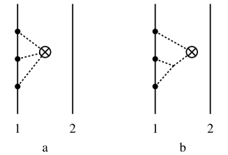
Figure 1: Dangerously divergent diagrams contributing to the 3PN multipole moments. The world-lines of particles 1 and 2 are represented by vertical solid lines, the propagator $\Box^{-1}$ by dotted lines, the source points by bullets, and the $\otimes$ symbol means a multiplication by a multipolar factor, such as $\hat{x}_{L}$, together with a spatial integration $\int d^{d}\mathbf{x}$.

Since the dangerous divergencies associated with the vicinity of the first world-line (say) are entirely contained in the diagrams shown in Fig. 1, they are, therefore, proportional to $m_{1}^{3}$ (i.e., one factor $m_{1}$ per source point), without any explicit  dependence on the second mass $m_{2}$. As a consequence, we can prove [19], because the presence of ambiguity parameters is directly linked with the occurence of poles $\propto 1/\varepsilon$, that the structure of the ambiguous terms in the mass quadrupole moment (4.1) must be such that it is proportional to some factor $m_{1}^{3}$. Now, the definition of the parameter $\kappa$ in Ref. [12] was to parametrize a conceivable a priori static ambiguity appearing in the renormalization of the logarithmic divergencies of the quadrupole moment, and these ambiguities were found in Eq. (4.1) to be of the form $\left(\xi+\kappa\right)\,m_{1}^{3}+\kappa\,m_{1}^{2}\,m_{2}$ (for what concerns the first particle). This shows that the parameter $\kappa$ corresponds to a mixing between diagrams with three legs on the first world-line (as in Fig. 1) and diagrams having two legs on the first world-line and one on the second. Our diagrammatic study has shown that the latter diagrams have no dangerous divergencies, i.e., that they do not introduce any conceivable ambiguity. Therefore we conclude, confirming Eq. (6), that

$$\kappa=0\,.$$ (30)

5 Field generated by a single body

As another application, making use of the explicit surface-integral formula (24), and yielding another check of ambiguity parameters, we wish to compute the source-type multipole moments of a spherically symmetric extended body moving with uniform velocity. Remember that our formalism assumes, in principle, that we are dealing with regular, weakly self-gravitating bodies. We expect, because of the effacing properties of Einstein’s theory [22], that our final physical results, especially when they are expressed as surface integrals like in (24), can be applied to more general sources, such as neutron stars or black holes. Indeed, we are going to confirm this expectation in the simplest possible case, that of an isolated spherically symmetric body which is known, by Birkhoff’s theorem, to generate a universal exterior gravitational field, given by the Schwarzschild solution.

5.1 The boosted Schwarzschild solution

Following Ref. [29] we shall apply our formulas to a boosted Schwarzschild solution (BSS). Actually, in order to justify our use of the BSS (in standard harmonic coordinates), we must dispose of a small technicality. This technicality concerns the non-uniqueness of harmonic coordinates for the Schwarzschild solution, even under the assumption of stationarity (in the rest frame) and spherical symmetry. Indeed, under these assumptions, and starting from the usual Schwarzschild radial coordinate, say $r_{S}$, the (rest frame) radial coordinate of the most general harmonic coordinate system, say $r=k(r_{S})$, must satisfy the differential equation (see, e.g., Weinberg [31], page 181)

$$\frac{d}{dr_{S}}\left[\left(r_{S}^{2}-\frac{2\,GM}{c^{2}}\,r_{S}\right)\frac{dk}{dr_{S}}\right]=2\,k\,.$$ (31)

The standard solution of Eq. (31), which is considered in all textbooks such as [31], reads simply

$$r=k^{\mathrm{standard}}(r_{S})=r_{S}-\frac{GM}{c^{2}}\,.$$ (32)

In the black hole case, the solution (32) is the only one which is regular on the horizon, i.e. when $r_{S}=2GM/c^{2}$. However, in the case of the external metric of an extended spherically symmetric body, regularity on the horizon is not a relevant issue. What is relevant is that the solution of the external problem (31) be smoothly matched to a regular solution of the corresponding internal problem. As usual, this matching determines a unique solution everywhere. In general, this unique, everywhere regular, solution will correspond, in the exterior of the body, to a particular case of the general, two-parameter solution of the second-order differential equation (31). The latter is of the form

$$r=k^{\mathrm{general}}(r_{S})=C_{1}\left(r_{S}-\frac{GM}{c^{2}}\right)+C_{2}\,k_{2}(r_{S})\,,$$ (33)

where $k_{2}(r_{S})$ denotes the (uniquely defined) “radially decaying solution” of Eq. (31), and where $C_{1}$ and $C_{2}$ are two integration constants. Indeed, when considering the flat-space limit of Eq. (31), it is easily seen that there are two independent solutions which behave, when $r_{S}\rightarrow+\infty$, as $r_{S}$ and $r_{S}^{-2}$ respectively. An explicit expression for the decaying solution is 

$$k_{2}(r_{S})=\frac{1}{r_{S}^{2}}\,F\left(2,2,4,\frac{2\,GM}{c^{2}r_{S}}\right)\,.$$ (34)

We can always normalize $C_{1}$ to the value $C_{1}=1$. Then, with the above definitions, $C_{2}$ has the dimension of a length cubed. By considering in more detail the matching of the general solution of the harmonically relaxed Einstein equations at the 2PN level (see, e.g., the book by Fock [32], page 322), one easily finds that the second integration constant is of the order of $C_{2}\sim(GM/c^{2})^{2}\,a$, where $a$ denotes the radius of the extended body under consideration. It is also easily checked that the constant $C_{2}$ parametrizes, at the linearized order, a gauge vector of the form $\varphi^{i}\propto C_{2}\,\partial_{i}(1/r)$, and can thus be referred to as a “gauge parameter”.

Contrarily to the multipole moments of stationary sources, which are geometric invariants (and can be expressed as surface integrals on a sphere at spatial infinity), the source multipole moments defined in Ref. [28] (and re-expressed in Section 3 as surface integrals over spheres in some intermediate region, $a\ll r\ll c\,T$) are probably not geometric invariants. They are useful intermediate constructs, which allow one to compute physically invariant information, but their definition is linked to the choice of harmonic coordinates covering the source. There are also various gauge multipoles (denoted $\mathrm{W}_{L}$, $\mathrm{X}_{L}$, $\mathrm{Y}_{L}$, $\mathrm{Z}_{L}$ in Ref. [28]) which will influence, at some non-linear order, the values of the two sequences of physical multipoles: $\mathrm{I}_{L}$, $\mathrm{J}_{L}$. Therefore, one should expect that, at some non-linear order, the physical multipoles $\mathrm{I}_{L}$, $\mathrm{J}_{L}$ of a boosted general, harmonic-coordinate spherically symmetric metric will start to depend on the value of the gauge parameter $C_{2}$.

Here, we are only interested in computing the quadrupole moment $\mathrm{I}_{ij}$ of a boosted general spherically symmetric metric. We shall see below that the index structure of $\mathrm{I}_{ij}$ will be provided by the STF tensor product of the boost velocity $V^{i}$ with itself, denoted $V^{\langle i}V^{j\rangle}$ (assuming that the origin of the coordinates is at the initial position of the center of symmetry of the BSS). Therefore, any contribution to $\mathrm{I}_{ij}$ coming from the gauge parameter $C_{2}$ must contain, at least, the factors $C_{2}$ and $V^{\langle i}V^{j\rangle}$, and also the total mass $M$. Taking into account the dimensionality of $C_{2}\sim(GM/c^{2})^{2}\,a$, which is that of a length cubed, it is easily seen that there is no way to generate such a contribution to $\mathrm{I}_{ij}$. Therefore, we conclude that the source quadrupole moment of a boosted general, harmonic-coordinate spherically symmetric metric is strictly equal to the source quadrupole moment of a boosted standard harmonic-coordinate Schwarzschild solution, obtained by setting $C_{2}=0$ (and $C_{1}=1$) in (33), i.e. by choosing the standard harmonic radial coordinate (32).

In the following, we shall therefore consider only such a boosted Schwarzschild solution (BSS) in standard form. We shall sometimes refer to the source of this solution as a black hole (though, strictly speaking, one should always have in mind some extended spherical star). For simplicity, we shall translate the origin of the coordinate system so that it is located at the initial position of the black hole at coordinate time $t=0$. With this choice of origin of the coordinates all the current-type moments $\mathrm{J}_{L}$ of the BSS are zero. We shall concentrate our attention on the mass-type quadrupole moment $\mathrm{I}_{ij}$, that we shall compute at the 3PN order.

The BSS metric, written in terms of the Gothic metric deviation $h^{\mu\nu}=\sqrt{-g}\,g^{\mu\nu}-\eta^{\mu\nu}$, satisfying standard harmonic coordinates so $\partial_{\nu}h^{\mu\nu}=0$, is best formulated in a manifestly Lorentz covariant way as

$$h^{\mu\nu}=\left(1-\frac{\left(1+\frac{G\,M}{c^{2}\,r_{\perp}}\right)^{3}}{1-\frac{G\,M}{c^{2}\,r_{\perp}}}\right)u^{\mu}u^{\nu}-\frac{G^{2}\,M^{2}}{c^{4}\,r_{\perp}^{2}}\,n^{\mu}n^{\nu}\,,$$ (35)

where $u^{\mu}$ is the time-like unit four-velocity of the center of symmetry of the BSS, where $n^{\mu}$ is the space-like unit vector pointing from the BSS to the field point along the direction orthogonal (in a Minkowskian sense) to the world line of the BSS, and where $r_{\perp}$ denotes the orthogonal distance to the world line (square root of the interval). However, in our explicit calculations (done with the software Mathematica) it is preferable to employ a more “coordinate-rooted” formulation of the BSS metric, which is of course completely equivalent to (though less elegant than) Eq. (35).

Le us denote by $x^{\mu}=(c\,t,\mathbf{x})$ the global reference frame, in which the black hole is moving, and by $X^{\mu}=(c\,T,\mathbf{X})$ the rest frame of the black hole — both $x^{\mu}$ and $X^{\mu}$ are assumed to be harmonic coordinates. Let $x^{i}(t)$ be the rectilinear and uniform trajectory of the center of symmetry of the BSS in the global coordinates $x^{\mu}$, and $\mathbf{V}=(V^{i})$ be the constant coordinate velocity of the BSS,

$$V^{i}\equiv\frac{dx^{i}(t)}{dt}\,.$$ (36)

The rest frame $X^{\mu}$ is transformed from the global one $x^{\mu}$ by the Lorentz boost,

$$x^{\mu}=\Lambda^{\mu}_{~{}\nu}(\mathbf{V})\,X^{\nu}\,.$$ (37)

For simplicity we consider a pure Lorentz boost $\Lambda^{\mu}_{~{}\nu}(\mathbf{V})$ without rotation of the spatial coordinates. As explained above, we can assume that the metric of the BSS in the rest frame $X^{\mu}$ takes the standard harmonic-coordinate Schwarzschild expression, which we write in terms of the Gothic metric deviation $H^{\mu\nu}$, satisfying $\partial_{\nu}H^{\mu\nu}=0$. Hence,

$$H^{00} = 1-\frac{\left(1+\frac{G\,M}{c^{2}\,R}\right)^{3}}{1-\frac{G\,M}{c^{2}\,R}}\,,$$ (38)

$$H^{i0} = 0\,,$$ (39)

$$H^{ij} = -\frac{G^{2}\,M^{2}}{c^{4}\,R^{2}}\,N^{i}N^{j}\,,$$ (40)

where $M$ is the total mass, $R\equiv|\mathbf{X}|$ and $N^{i}\equiv X^{i}/R$. A well-known feature of the Schwarzschild metric in harmonic coordinates is that the spatial Gothic metric $H^{ij}$ is made of a single quadratic-order term $\propto G^{2}$ as shown in Eq. (40). The Gothic metric deviation transforms like a Lorentz tensor so the metric of the BSS in the global frame $x^{\mu}$ reads as

$$h^{\mu\nu}(x)=\Lambda^{\mu}_{~{}~{}\rho}\Lambda^{\nu}_{~{}~{}\sigma}\,H^{\rho\sigma}(\Lambda^{-1}x)\,,$$ (41)

in which the rest-frame coordinates have been expressed by means of the global ones, i.e. $X^{\mu}(x)=(\Lambda^{-1})^{\mu}_{~{}\nu}x^{\nu}$, using the inverse Lorentz transformation. The only problem is to derive the explicit relations giving the rest-frame radial coordinate $R$ and the unit direction $N^{i}$ as functions of their global-frame counterparts $r$ and $n^{i}$, of the global coordinate time $t$, and of the boost velocity $V^{i}$. For these relations we find

$$R = r\,\biggl{[}1+c^{2}(\gamma^{2}-1)\left(\frac{t}{r}\right)^{2}-2\gamma^{2}(Vn)\left(\frac{t}{r}\right)+\gamma^{2}\frac{(Vn)^{2}}{c^{2}}\biggr{]}^{1/2}\,,$$ (42)

$$N^{i} = \frac{r}{R}\left[n^{i}-\gamma V^{i}\left(\frac{t}{r}\right)+\frac{\gamma^{2}}{\gamma+1}\frac{V^{i}}{c^{2}}(Vn)\right]\,,$$ (43)

where $\gamma\equiv\left(1-V^{2}/c^{2}\right)^{-1/2}$ and $(Vn)\equiv\mathbf{V}\cdot\mathbf{n}=V^{j}n^{j}$ is the usual Euclidean scalar product. The latter formulation of the BSS metric is well adapted to our calculations because we shall have to perform, for computing the source multipole moments, an integration over the coordinate three-dimensional spatial slice $\mathbf{x}\in\mathbb{R}^{3}$, with coordinate time $t=\mathrm{const}$, which is easily done using the explicit relations (42)–(43).

5.2 Quadrupole moment of a boosted Schwarzschild black hole

We compute the quadrupole moment $\mathrm{I}_{ij}$ of the BSS, following the prescriptions defined by Eq. (24). To this end we first expand $h^{\mu\nu}$ when $c\rightarrow+\infty$, taking into account all the $c$’s present both in the expression of the rest frame metric $H^{\mu\nu}$ as well as those coming from the Lorentz transformation (41)–(43). In this process the boost velocity $\mathbf{V}$ is to be considered as a constant, “spectator”, vector. Note in passing that, in the present problem, the characteristic size $a$ of the source at time $t$ is given by the displacement from the origin, $a\sim V\,t$, where $V\equiv|\mathbf{V}|$, while the near-zone corresponds to $r\ll c\,t$. Therefore, the far near-zone, where we read off the multipole moments as some combination of expansion coefficients $\varphi_{a,b}^{\mu\nu}(\mathbf{n},t)$, is the domain $V\,t\ll r\ll c\,t$. We have evidently to assume that $V\ll c$ for this region to exist.

We then first get the near-zone (or PN) expansion of the BSS metric, $\overline{h}^{\mu\nu}$, by expanding in inverse powers of $c$ up to 3PN order. Next we compute the multipolar (or far) re-expansion of each of the PN coefficients when $r\rightarrow+\infty$ with $t=\mathrm{const}$. In this way we obtain what we have denoted by $\mathcal{M}\bigl{(}\overline{h}^{\mu\nu}\bigr{)}$ in Eq. (17). In the BBS case it is evident that the far-zone expansion given by (17) involves simply some powers of $1/r$, without any logarithm of $r$.

With $\mathcal{M}\bigl{(}\overline{h}^{\mu\nu}\bigr{)}$ in hand we have the coefficients of the various powers of $1/r$, and we obtain thereby the needed quantities $\Psi_{k,\ell}^{\mu\nu}$ defined by Eq. (21). It is then a simple matter to compute all the required angular averages present in the formula (24) and to obtain the following 3PN mass quadrupole moment of the BSS,

$$\mathrm{I}_{ij}^{\mathrm{\,BSS}} = M\,t^{2}\,V^{\langle i}V^{j\rangle}\left[1+\frac{9}{14}\,\frac{V^{2}}{c^{2}}+\frac{83}{168}\,\frac{V^{4}}{c^{4}}+\frac{507}{1232}\,\frac{V^{6}}{c^{6}}\right]$$ (44)

$$+ \frac{4}{7}\,\frac{G^{2}\,M^{3}}{c^{6}}\,V^{\langle i}V^{j\rangle}+\mathcal{O}\left(\frac{1}{c^{8}}\right)\,.$$

The first term represents the standard Newtonian expression, augmented here by a bunch of relativistic corrections. (Recall that we have chosen the origin of the coordinate system at the initial location of the BSS at $t=0$.)

The last term in Eq. (44), with coefficient $\mathcal{C}=4/7$, is the most interesting for our purpose. It is purely of 3PN order, and it contains the first occurence of the gravitational constant $G$, which therefore arises in the quadrupole of the BSS only at 3PN order. This term is interesting because it corresponds to one of the regularization ambiguities, due to an incompleteness of Hadamard’s self-field regularization, which appears in the calculation of the mass-type quadrupole moment of point particle binaries at the 3PN order [12, 13]. As we see from Eq. (4.1) the associated ambiguity parameter is $\zeta$, which represents in fact the analogue of the kinetic ambiguity parameter $\omega_{\mathrm{kinetic}}$ in the equations of motion, see Eq. (1). It is now clear that $\zeta$ can be determined from what we shall now call the BSS limit of a binary system, which consists of setting one of the masses of the binary to be exactly zero, say $m_{2}=0$.

We have obtained the BSS limit of the 3PN mass-type quadrupole moment of compact binaries computed for general binary orbits in Refs. [12, 13]. We have also inserted for the position of the first body $y_{1}^{i}=v_{1}^{i}\,t$ in order to conform with our choice for the origin of the coordinates. In this way we get

$$\mathrm{I}_{ij}^{\mathrm{\,BSS\,limit}} = m_{1}\,t^{2}\,v_{1}^{\langle i}v_{1}^{j\rangle}\left[1+\frac{9}{14}\,\frac{v_{1}^{2}}{c^{2}}+\frac{83}{168}\,\frac{v_{1}^{4}}{c^{4}}+\frac{507}{1232}\,\frac{v_{1}^{6}}{c^{6}}\right]$$ (45)

$$+ \biggl{(}\frac{232}{63}+\frac{44}{3}\zeta\biggr{)}\frac{G^{2}\,m_{1}^{3}}{c^{6}}\,v_{1}^{\langle i}v_{1}^{j\rangle}+\mathcal{O}\left(\frac{1}{c^{8}}\right)\,.$$

The comparison of Eqs. (45) and (44) reveals a complete match between the two results if and only if we have the expected agreement between the masses, i.e. $M=m_{1}$, and the velocities, $v_{1}^{i}=V^{i}$ (since the velocity of the body remaining after taking the BSS limit should exactly be the boost velocity), and the ambiguity constant $\zeta$ takes the unique value

$$\zeta=-\frac{7}{33}\,.$$ (46)

Our conclusion, therefore, is that the ambiguity parameter $\zeta$ is uniquely determined by the BSS limit. Because of the close relation between the BSS limit with Lorentz boosts, it is clear that $\zeta$ is linked to the Lorentz-Poincaré invariance of the multipole moment formalism of Ref. [28] as applied to compact binary systems in [12, 13]. This link strongly suggests that the specific value (46) represents the only one for which the expression of the 3PN quadrupole moment is compatible with the Poincaré symmetry. In other words the present calculation indicates that the Poincaré invariance should correctly be incorporated into the laws of transformation of the source-type multipole moments for general extended PN sources as given by Eqs. (10)–(11) or (24)–(25).

Let us finally emphasize that Eq. (46) has been obtained here without using any regularization scheme for curing the divergencies associated with the self field of point particles. However, we find, very nicely, that the value for $\zeta$ is in agreement with the one derived in the problem of point particles binaries at 3PN order by means of the dimensional self-field regularization, Eq. (7). This shows in particular that dimensional regularization is able to correctly keep track of the global Poincaré invariance of the general relativistic description of isolated systems.

References

- [1] C. Cutler, T.A. Apostolatos, L. Bildsten, L.S. Finn, E.E. Flanagan, D. Kennefick, D.M. Markovic, A. Ori, E. Poisson, G.J. Sussman, and K.S. Thorne. The last three minutes: Issues in gravitational-wave measurements of coalescing compact binaries. Phys. Rev. Lett., 70:2984–2987, 1993.
- [2] C. Cutler and E.E. Flanagan. Gravitational waves from merging compact binaries: How accurately can one extract the binary’s parameters from the inspiral waveform? Phys. Rev. D, 49:2658–2697, 1994.
- [3] Luc Blanchet, Thibault Damour, Bala R. Iyer, Clifford M. Will, and Alan. G. Wiseman. Gravitational radiation damping of compact binary systems to second post-newtonian order. Phys. Rev. Lett., 74:3515–3518, 1995.
- [4] Luc Blanchet, Guillaume Faye, Bala R. Iyer, and Benoit Joguet. Gravitational-wave inspiral of compact binary systems to 7/2 post-newtonian order. Phys. Rev. D, 65:061501(R), 2002. Erratum Phys. Rev. D 71, 129902(E) (2005).
- [5] Luc Blanchet, Thibault Damour, Gilles Esposito-Farèse, and Bala R. Iyer. Gravitational radiation from inspiralling compact binaries completed at the third post-newtonian order. Phys. Rev. Lett., 93:091101, 2004.
- [6] P. Jaranowski and G. Schäfer. Third post-newtonian higher order adm hamilton dynamics for two-body point-mass systems. Phys. Rev. D, 57:7274–7291, 1998.
- [7] P. Jaranowski and G. Schäfer. Binary black-hole problem at the third post-newtonian approximation in the orbital motion: Static part. Phys. Rev. D, 60:124003–1–12403–7, 1999.
- [8] Luc Blanchet and Guillaume Faye. Equations of motion of point-particle binaries at the third post-newtonian order. Phys. Lett. A, 271:58, 2000.
- [9] Luc Blanchet and Guillaume Faye. General relativistic dynamics of compact binaries at the third post-newtonian order. Phys. Rev. D, 63:062005, 2001.
- [10] V.C. de Andrade, L. Blanchet, and G. Faye. Third post-newtonian dynamics of compact binaries: Noetherian conserved quantities and equivalence between the harmonic-coordinate and adm-hamiltonian formalisms. Class. Quant. Grav., 18:753–778, 2001.
- [11] Luc Blanchet. Gravitational-wave tails of tails. Class. Quant. Grav., 15:113–141, 1998. Erratum Class. Quant. Grav. 22, 3381 (2005).
- [12] Luc Blanchet, Bala R. Iyer, and Benoit Joguet. Gravitational waves from inspiralling compact binaries: Energy flux to third post-newtonian order. Phys. Rev. D, 65:064005, 2002. Erratum Phys. Rev. D 71, 129903(E) (2005).
- [13] Luc Blanchet and Bala R. Iyer. Hadamard regularization of the third post-newtonian gravitational wave generation of two point masses. Phys. Rev. D, 71:024004, 2004.
- [14] J. Hadamard. Le problème de Cauchy et les équations aux dérivées partielles linéaires hyperboliques. Hermann, Paris, 1932.
- [15] L. Schwartz. Théorie des distributions. Hermann, Paris, 1978.
- [16] G. ’t Hooft and M. Veltman. Nucl. Phys., B44:139, 1972.
- [17] T. Damour, P. Jaranowski, and G. Schäfer. Dimensional regularization of the gravitational interaction of point masses. Phys. Lett. B, 513:147–155, 2001.
- [18] Luc Blanchet, Thibault Damour, and Gilles Esposito-Farèse. Dimensional regularization of the third post-newtonian dynamics of point particles in harmonic coordinates. Phys. Rev. D, 69:124007, 2004.
- [19] Luc Blanchet, Thibault Damour, Gilles Esposito-Farèse, and Bala R. Iyer. Dimensional regularization of the third post-newtonian gravitational wave generation of two point masses. Phys. Rev. D, 71:124004, 2005.
- [20] Luc Blanchet and Guillaume Faye. Hadamard regularization. J. Math. Phys., 41:7675–7714, 2000.
- [21] Luc Blanchet and Guillaume Faye. Lorentzian regularization and the problem of point-like particles in general relativity. J. Math. Phys., 42:4391–4418, 2001.
- [22] T. Damour. Gravitational radiation and the motion of compact bodies. In N. Deruelle and T. Piran, editors, Gravitational Radiation, pages 59–144, Amsterdam, 1983. North-Holland Company.
- [23] S.M. Kopeikin. The equations of motion of extended bodies in general-relativity with conservative corrections and radiation damping taken into account. Astron. Zh., 62:889–904, 1985.
- [24] L.P. Grishchuk and S.M. Kopeikin. Equations of motion for isolated bodies with relativistic corrections including the radiation reaction force. In J. Kovalevsky and V.A. Brumberg, editors, Relativity in Celestial Mechanics and Astrometry, pages 19–33, Dordrecht, 1986. Reidel.
- [25] Yousuke Itoh and Toshifumi Futamase. Phys. Rev. D, 68:121501(R), 2003.
- [26] Yousuke Itoh. Phys. Rev. D, 69:064018, 2004.
- [27] A. Einstein, L. Infeld, and B. Hoffmann. The gravitational equations and the problem of motion. Ann. Math., 39:65–100, 1938.
- [28] Luc Blanchet. On the multipole expansion of the gravitational field. Class. Quant. Grav., 15:1971–1999, 1998.
- [29] Luc Blanchet, Thibault Damour, and Bala R. Iyer. Surface-integral expressions for the multipole moments of post-newtonian sources and the boosted schwarzschild solution. Class. Quant. Grav., 22:155, 2005.
- [30] Thibault Damour and Gilles Esposito-Farèse. Testing gravity to second post-newtonian order: A field theory approach. Phys. Rev. D, 53:5541–5578, 1996.
- [31] S. Weinberg. Gravitation and Cosmology. John Wiley, New York, 1972.
- [32] V.A. Fock. Theory of space, time and gravitation. Pergamon, London, 1959.