An introduction to relativistic hydrodynamics

Abstract

This lecture provides some introduction to perfect fluid dynamics within the framework of general relativity. The presentation is based on the Carter-Lichnerowicz approach. It has the advantage over the more traditional approach of leading very straightforwardly to important conservation laws, such as the relativistic generalizations of Bernoulli’s theorem or Kelvin’s circulation theorem. It also permits to get easily first integrals of motion which are particularly useful for computing equilibrium configurations of relativistic stars in rotation or in binary systems. The presentation is relatively self-contained and does not require any a priori knowledge of general relativity. In particular, the three types of derivatives involved in relativistic hydrodynamics are introduced in detail: this concerns the Lie, exterior and covariant derivatives.

1 Introduction

Relativistic fluid dynamics is an important topic of modern astrophysics in at least three contexts: (i) jets emerging at relativistic speed from the core of active galactic nuclei or from microquasars, and certainly from gamma-ray burst central engines, (ii) compact stars and flows around black holes, and (iii) cosmology. Notice that for items (ii) and (iii) general relativity is necessary, whereas special relativity is sufficient for (i).

We provide here an introduction to relativistic perfect fluid dynamics in the framework of general relativity, so that it is applicable to all themes (i) to (iii). However, we shall make a limited usage of general relativistic concepts. In particular, we shall not use the Riemannian curvature and all the results will be independent of the Einstein equation.

We have chosen to introduce relativistic hydrodynamics via an approach developed originally by Lichnerowicz ([1941], [1955], [1967]) and extended significantly by Carter ([1973], [1979], [1989]). This formulation is very elegant and permits an easy derivation of the relativistic generalizations of all the standard conservation laws of classical fluid mechanics. Despite of this, it is absent from most (all ?) textbooks. The reason may be that the mathematical settings of Carter-Lichnerowicz approach is Cartan’s exterior calculus, which departs from what physicists call “standard tensor calculus”. Yet Cartan’s exterior calculus is simpler than the “standard tensor calculus” for it does not require any specific structure on the spacetime manifold. In particular, it is independent of the metric tensor and its associated covariant derivation, not speaking about the Riemann curvature tensor. Moreover it is well adapted to the computation of integrals and their derivatives, a feature which is obviously important for hydrodynamics.

Here we start by introducing the general relativistic spacetime as a pretty simple mathematical structure (called manifold) on which one can define vectors and multilinear forms. The latter ones map vectors to real numbers, in a linear way. The differential forms on which Cartan’s exterior calculus is based are then simply multilinear forms that are fully antisymmetric. We shall describe this in Sec. 2, where we put a special emphasis on the definition of the three kinds of derivative useful for hydrodynamics: the exterior derivative which acts only on differential forms, the Lie derivative along a given vector field and the covariant derivative which is associated with the metric tensor. Then in Sec. 3 we move to physics by introducing the notions of particle worldline, proper time, 4-velocity and 4-acceleration, as well as Lorentz factor between two observers. The hydrodynamics then starts in Sec. 4 where we introduce the basic object for the description of a fluid: a bilinear form called the stress-energy tensor. In this section, we define also the concept of perfect fluid and that of equation of state. The equations of fluid motion are then deduced from the local conservation of energy and momentum in Sec. 5. They are given there in the standard form which is essentially a relativistic version of Euler equation. From this standard form, we derive the Carter-Lichnerowicz equation of motion in Sec. 6, before specializing it to the case of an equation of state which depends on two parameters: the baryon number density and the entropy density. We also show that the Newtonian limit of the Carter-Lichnerowicz equation is a well known alternative form of the Euler equation, namely the Crocco equation. The power of the Carter-Lichnerowicz approach appears in Sec. 7 where we realize how easy it is to derive conservation laws from it, among which the relativistic version of the classical Bernoulli theorem and Kelvin’s circulation theorem. We also show that some of these conservation laws are useful for getting numerical solutions for rotating relativistic stars or relativistic binary systems.

2 Fields and derivatives in spacetime

It is not the aim of this lecture to provide an introduction to general relativity. For this purpose we refer the reader to two excellent introductory textbooks which have recently appeared: (Hartle [2003]) and (Carrol [2004]). Here we recall only some basic geometrical concepts which are fundamental to a good understanding of relativistic hydrodynamics. In particular we focus on the various notions of derivative on spacetime.

2.1 The spacetime of general relativity

Relativity has performed the fusion of space and time, two notions which were completely distinct in Newtonian mechanics. This gave rise to the concept of spacetime, on which both the special and general theory of relativity are based. Although this is not particularly fruitful (except for contrasting with the relativistic case), one may also speak of spacetime in the Newtonian framework. The Newtonian spacetime $\mathcal{M}$ is then nothing but the affine space $\mathbb{R}^{4}$, foliated by the hyperplanes $\Sigma_{t}$ of constant absolute time $t$: these hyperplanes represent the ordinary 3-dimensional space at successive instants. The foliation $(\Sigma_{t})_{t\in\mathbb{R}}$ is a basic structure of the Newtonian spacetime and does not depend upon any observer. The worldline $\mathcal{L}$ of a particle is the curve in $\mathcal{M}$ generated by the successive positions of the particle. At any point $A\in\mathcal{L}$, the time read on a clock moving along $\mathcal{L}$ is simply the parameter $t$ of the hyperplane $\Sigma_{t}$ that intersects $\mathcal{L}$ at $A$.

The spacetime $\mathcal{M}$ of special relativity is the same mathematical space as the Newtonian one, i.e. the affine space $\mathbb{R}^{4}$. The major difference with the Newtonian case is that there does not exist any privileged foliation $(\Sigma_{t})_{t\in\mathbb{R}}$. Physically this means that the notion of absolute time is absent in special relativity. However $\mathcal{M}$ is still endowed with some absolute structure: the metric tensor $\bm{g}$ and the associated light cones. The metric tensor is a symmetric bilinear form $\bm{g}$ on $\mathcal{M}$, which defines the scalar product of vectors. The null (isotropic) directions of $\bm{g}$ give the worldlines of photons (the light cones). Therefore these worldlines depend only on the absolute structure $\bm{g}$ and not, for instance, on the observer who emits the photon.

The spacetime $\mathcal{M}$ of general relativity differs from both Newtonian and special relativistic spacetimes, in so far as it is no longer the affine space $\mathbb{R}^{4}$ but a more general mathematical structure, namely a manifold. A manifold of dimension 4 is a topological space such that around each point there exists a neighbourhood which is homeomorphic to an open subset of $\mathbb{R}^{4}$. This simply means that, locally, one can label the points of $\mathcal{M}$ in a continuous way by 4 real numbers $(x^{\alpha})_{\alpha\in\{0,1,2,3\}}$ (which are called coordinates). To cover the full $\mathcal{M}$, several different coordinates patches (charts in mathematical jargon) can be required.

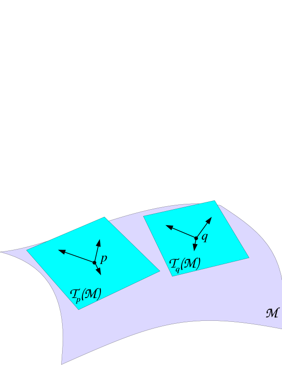
Figure 1: The vectors at two points $p$ and $q$ on the spacetime manifold $\mathcal{M}$ belong to two different vector spaces: the tangent spaces $\mathcal{T}_{p}(\mathcal{M})$ and $\mathcal{T}_{q}(\mathcal{M})$.

Within the manifold structure the definition of vectors is not as trivial as within the affine structure of the Newtonian and special relativistic spacetimes. Indeed, only infinitesimal vectors connecting two infinitely close points can be defined a priori on a manifold. At a given point $p\in\mathcal{M}$, the set of such vectors generates a 4-dimensional vector space, which is called the tangent space at the point $p$ and is denoted by $\mathcal{T}_{p}(\mathcal{M})$. The situation is therefore different from the Newtonian or special relativistic one, for which the very definition of an affine space provides a unique global vector space. On a manifold there are as many vector spaces as points $p$ (cf. Fig. 1).

Given a vector basis $(\vec{\bm{e}}_{\alpha})_{\alpha\in\{0,1,2,3\}}$ of $\mathcal{T}_{p}(\mathcal{M})$, the components of a vector $\vec{\bm{v}}\in\mathcal{T}_{p}(\mathcal{M})$ on this basis are denoted by $v^{\alpha}$: $\vec{\bm{v}}=v^{\alpha}\vec{\bm{e}}_{\alpha}$, where we have employed Einstein’s convention for summation on repeated indices. It happens frequently that the vector basis is associated to a coordinate system $(x^{\alpha})$ on the manifold, in the following way. If $dx^{\alpha}$ is the (infinitesimal) difference of coordinates between $p$ and a neighbouring point $q$, the components of the vector $\overrightarrow{pq}$ with respect to the basis $(\vec{\bm{e}}_{\alpha})$ are exactly $dx^{\alpha}$. The basis that fulfills this property is unique and is called the natural basis associated with the coordinate system $(x^{\alpha})$. It is usually denoted by $(\partial/\partial x^{\alpha})$, which is a reminiscence of the intrinsic definition of vectors on a manifold as differential operators acting on scalar fields.

As for special relativity, the absolute structure given on the spacetime manifold $\mathcal{M}$ of general relativity is the metric tensor $\bm{g}$. It is now a field on $\mathcal{M}$: at each point $p\in\mathcal{M}$, $\bm{g}(p)$ is a symmetric bilinear form acting on vectors in the tangent space $\mathcal{T}_{p}(\mathcal{M})$:

$$\begin{array}[]{rccl}\bm{g}(p):&\mathcal{T}_{p}(\mathcal{M})\times\mathcal{T}_{p}(\mathcal{M})&\longrightarrow&\mathbb{R}\\ &(\vec{\bm{u}},\vec{\bm{v}})&\longmapsto&\bm{g}(\vec{\bm{u}},\vec{\bm{v}})=:\vec{\bm{u}}\cdot\vec{\bm{v}}.\end{array}$$ (1)

It is demanded that the bilinear form $\bm{g}$ is not degenerate and is of signature $(-,+,+,+)$. It thus defines a scalar product on $\mathcal{T}_{p}(\mathcal{M})$, which justifies the notation $\vec{\bm{u}}\cdot\vec{\bm{v}}$ for $\bm{g}(\vec{\bm{u}},\vec{\bm{v}})$. The isotropic directions of $\bm{g}$ give the local light cones: a vector $\vec{\bm{v}}\in\mathcal{T}_{p}(\mathcal{M})$ is tangent to a light cone and called a null or lightlike vector iff $\vec{\bm{v}}\cdot\vec{\bm{v}}=0$. Otherwise, the vector is said to be timelike iff $\vec{\bm{v}}\cdot\vec{\bm{v}}<0$ and spacelike iff $\vec{\bm{v}}\cdot\vec{\bm{v}}>0$.

2.2 Tensors

Let us recall that a linear form at a given point $p\in\mathcal{M}$ is an application

$$\begin{array}[]{rccl}\bm{\omega}:&\mathcal{T}_{p}(\mathcal{M})&\longrightarrow&\mathbb{R}\\ &\vec{\bm{v}}&\longmapsto&\langle\bm{\omega},\vec{\bm{v}}\rangle:=\bm{\omega}(\vec{\bm{v}}),\end{array}$$ (2)

that is linear. The set of all linear forms at $p$ forms a vector space of dimension 4, which is denoted by $\mathcal{T}_{p}(\mathcal{M})^{*}$ and is called the dual of the tangent space $\mathcal{T}_{p}(\mathcal{M})$. In relativistic physics, an abundant use is made of linear forms and their generalizations: the tensors. A tensor of type $(k,\ell)$, also called tensor $k$ times contravariant and $\ell$ times covariant, is an application

$$\begin{array}[]{rccl}\bm{T}:&\underbrace{\mathcal{T}_{p}(\mathcal{M})^{*}\times\cdots\times\mathcal{T}_{p}(\mathcal{M})^{*}}_{k{\ \rm times}}\times\underbrace{\mathcal{T}_{p}(\mathcal{M})\times\cdots\times\mathcal{T}_{p}(\mathcal{M})}_{\ell{\ \rm times}}&\longrightarrow&\mathbb{R}\\ &(\bm{\omega}_{1},\ldots,\bm{\omega}_{k},\vec{\bm{v}}_{1},\ldots,\vec{\bm{v}}_{\ell})&\longmapsto&\bm{T}(\bm{\omega}_{1},\ldots,\bm{\omega}_{k},\\ &&&\ \quad\vec{\bm{v}}_{1},\ldots,\vec{\bm{v}}_{\ell})\end{array}$$ (3)

that is linear with respect to each of its arguments. The integer $k+\ell$ is called the valence of the tensor. Let us recall the canonical duality $\mathcal{T}_{p}(\mathcal{M})^{**}=\mathcal{T}_{p}(\mathcal{M})$, which means that every vector $\vec{\bm{v}}$ can be considered as a linear form on the space $\mathcal{T}_{p}(\mathcal{M})^{*}$, defining the application $\vec{\bm{v}}:\;\mathcal{T}_{p}(\mathcal{M})^{*}\rightarrow\mathbb{R}$, $\bm{\omega}\mapsto\langle\bm{\omega},\vec{\bm{v}}\rangle$. Accordingly a vector is a tensor of type $(1,0)$. A linear form is a tensor of type $(0,1)$ and the metric tensor $\bm{g}$ is a tensor of type $(0,2)$.

Let us consider a vector basis of $\mathcal{T}_{p}(\mathcal{M})$, $(\vec{\bm{e}}_{\alpha})$, which can be either a natural basis (i.e. related to some coordinate system) or not (this is often the case for bases orthonormal with respect to the metric $\bm{g}$). There exists then a unique quadruplet of 1-forms, $(\bm{e}^{\alpha})$, that constitutes a basis of the dual space $\mathcal{T}_{p}(\mathcal{M})^{*}$ and that verifies

$$\langle\bm{e}^{\alpha},\vec{\bm{e}}_{\beta}\rangle=\delta^{\alpha}_{\ \,\beta},$$ (4)

where $\delta^{\alpha}_{\ \,\beta}$ is the Kronecker symbol. Then we can expand any tensor $\bm{T}$ of type $(k,\ell)$ as

$$\framebox{$\displaystyle\bm{T}=T^{\alpha_{1}\ldots\alpha_{k}}_{\qquad\ \;\beta_{1}\ldots\beta_{\ell}}\;\vec{\bm{e}}_{\alpha_{1}}\otimes\ldots\otimes\vec{\bm{e}}_{\alpha_{k}}\otimes\bm{e}^{\beta_{1}}\otimes\ldots\otimes\bm{e}^{\beta_{\ell}}$},$$ (5)

where the tensor product $\vec{\bm{e}}_{\alpha_{1}}\otimes\ldots\otimes\vec{\bm{e}}_{\alpha_{k}}\otimes\bm{e}^{\beta_{1}}\otimes\ldots\otimes\bm{e}^{\beta_{\ell}}$ is the tensor of type $(k,\ell)$ for which the image of $(\bm{\omega}_{1},\ldots,\bm{\omega}_{k},\vec{\bm{v}}_{1},\ldots,\vec{\bm{v}}_{\ell})$ as in (3) is the real number

$$\prod_{i=1}^{k}\langle\bm{\omega}_{i},\vec{\bm{e}}_{\alpha_{i}}\rangle\;\times\;\prod_{j=1}^{\ell}\langle\bm{e}^{\beta_{j}},\vec{\bm{v}}_{j}\rangle.$$ (6)

Notice that all the products in the above formula are simply products in $\mathbb{R}$. The $4^{k+\ell}$ scalar coefficients $T^{\alpha_{1}\ldots\alpha_{k}}_{\qquad\ \;\beta_{1}\ldots\beta_{\ell}}$ in (5) are called the components of the tensor $\bm{T}$ with respect to the basis $(\vec{\bm{e}}_{\alpha})$, or with respect to the coordinates $(x^{\alpha})$ if $(\vec{\bm{e}}_{\alpha})$ is the natural basis associated with these coordinates. These components are unique and fully characterize the tensor $\bm{T}$. Actually, in many studies, a basis is assumed (mostly a natural basis) and the tensors are always represented by their components. This way of presenting things is called the index notation, or the abstract index notation if the basis is not specified (e.g. Wald [1984]). We shall not use it here, sticking to what is called the index-free notation and which is much better adapted to exterior calculus and Lie derivatives.

The notation $v^{\alpha}$ already introduced for the components of a vector $\vec{\bm{v}}$ is of course the particular case $(k=1,\ell=0)$ of the general definition given above. For a linear form $\bm{\omega}$, the components $\omega_{\alpha}$ are such that $\bm{\omega}=\omega_{\alpha}\bm{e}^{\alpha}$ [Eq. (5) with $(k=0,\ell=1)$]. Then

$$\langle\bm{\omega},\vec{\bm{v}}\rangle=\omega_{\alpha}v^{\alpha}.$$ (7)

Similarly the components $g_{\alpha\beta}$ of the metric tensor $\bm{g}$ are defined by $\bm{g}=g_{\alpha\beta}\,\bm{e}^{\alpha}\otimes\bm{e}^{\beta}$ [Eq. (5) with $(k=0,\ell=2)$] and the scalar products are expressed in terms of the components as

$$\bm{g}(\vec{\bm{u}},\vec{\bm{v}})=g_{\alpha\beta}u^{\alpha}v^{\beta}.$$ (8)

2.3 Scalar fields and their gradients

A scalar field on the spacetime manifold $\mathcal{M}$ is an application $f:\ \mathcal{M}\rightarrow\mathbb{R}$. If $f$ is smooth, it gives rise to a field of linear forms (such fields are called 1-forms), called the gradient of $f$ and denoted $\bm{\mathrm{d}}f$. It is defined so that the variation of $f$ between two neighbouring points $p$ and $q$ is

$$df=f(q)-f(p)=\langle\bm{\mathrm{d}}f,\overrightarrow{pq}\rangle.$$ (9)

Let us note that, in non-relativistic physics, the gradient is very often considered as a vector and not as a 1-form. This is because one associates implicitly a vector $\vec{\omega}$ to any 1-form $\omega$ thanks to the Euclidean scalar product of $\mathbb{R}^{3}$, via $\forall\vec{v}\in\mathbb{R}^{3},\ \langle\omega,\vec{v}\rangle=\vec{\omega}\cdot\vec{v}$. Accordingly, the formula (9) is rewritten as $df=\vec{\nabla}f\cdot\overrightarrow{pq}$. But one shall keep in mind that, fundamentally, the gradient is a 1-form and not a vector.

If $(x^{\alpha})$ is a coordinate system on $\mathcal{M}$ and $(\vec{\bm{e}}_{\alpha}=\partial/\partial x^{\alpha})$ the associated natural basis, then the dual basis is constituted by the gradients of the four coordinates: $\bm{e}^{\alpha}=\bm{\mathrm{d}}x^{\alpha}$. The components of the gradient of any scalar field $f$ in this basis are then nothing but the partial derivatives of $f$:

$$\bm{\mathrm{d}}f=(\bm{\mathrm{d}}f)_{\alpha}\,\bm{\mathrm{d}}x^{\alpha}\qquad\mbox{with}\qquad(\bm{\mathrm{d}}f)_{\alpha}=\frac{\partial f}{\partial x^{\alpha}}.$$ (10)

2.4 Comparing vectors and tensors at different spacetime points: various derivatives on $\mathcal{M}$

A basic concept for hydrodynamics is of course that of vector field. On the manifold $\mathcal{M}$, this means the choice of a vector $\vec{\bm{v}}(p)$ in $\mathcal{T}_{p}(\mathcal{M})$ for each $p\in\mathcal{M}$. We denote by $\mathcal{T}(\mathcal{M})$ the space of all smooth vector fields on $\mathcal{M}$ . The derivative of the vector field is to be constructed for the variation $\delta\vec{\bm{v}}$ of $\vec{\bm{v}}$ between two neighbouring points $p$ and $q$. Naively, one would write $\delta\vec{\bm{v}}=\vec{\bm{v}}(q)-\vec{\bm{v}}(p)$, as in (9). However $\vec{\bm{v}}(q)$ and $\vec{\bm{v}}(p)$ belong to different vector spaces: $\mathcal{T}_{q}(\mathcal{M})$ and $\mathcal{T}_{p}(\mathcal{M})$ (cf. Fig. 1). Consequently the subtraction $\vec{\bm{v}}(q)-\vec{\bm{v}}(p)$ is ill defined, contrary of the subtraction of two real numbers in (9). To proceed in the definition of the derivative of a vector field, one must introduce some extra-structure on the manifold $\mathcal{M}$: this can be either another vector field $\vec{\bm{u}}$, leading to the derivative of $\vec{\bm{v}}$ along $\vec{\bm{u}}$ which is called the Lie derivative, or a connection $\bm{\nabla}$ (usually related to the metric tensor $\bm{g}$), leading to the covariant derivative $\bm{\nabla}\vec{\bm{v}}$. These two types of derivative generalize straightforwardly to any kind of tensor field. For the specific kind of tensor fields constituted by differential forms, there exists a third type of derivative, which does not require any extra structure on $\mathcal{M}$: the exterior derivative. We will discuss the latter in Sec. 2.5. In the current section, we shall review successively the Lie and covariant derivatives.

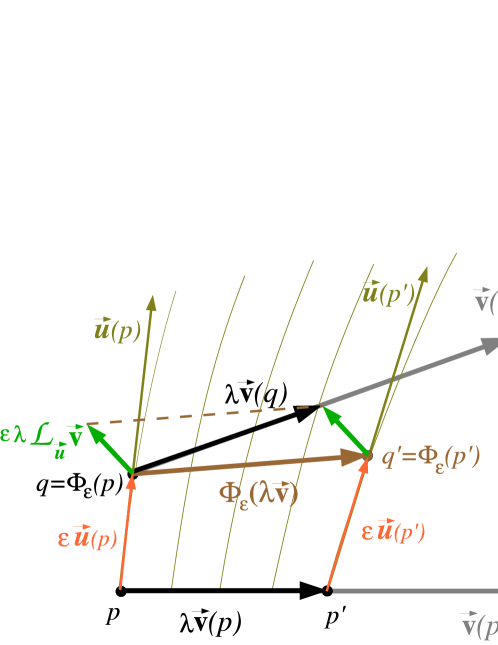
Figure 2: Geometrical construction of the Lie derivative of a vector field: given a small parameter $\lambda$, each extremity of the arrow $\lambda\vec{\bm{v}}$ is dragged by some small parameter $\varepsilon$ along $\vec{\bm{u}}$, to form the vector denoted by $\Phi_{\varepsilon}(\lambda\vec{\bm{v}})$. The latter is then compared with the actual value of $\lambda\vec{\bm{v}}$ at the point $q$, the difference (divided by $\lambda\varepsilon$) defining the Lie derivative $\bm{\mathcal{L}}_{\vec{\bm{u}}}\,\vec{\bm{v}}$.

2.4.1 Lie derivative

The Lie derivative is a very natural operation in the context of fluid mechanics. Indeed, consider a vector field $\vec{\bm{u}}$ on $\mathcal{M}$, called hereafter the flow. Let $\vec{\bm{v}}$ be another vector field on $\mathcal{M}$, the variation of which is to be studied. We can use the flow $\vec{\bm{u}}$ to transport the vector $\vec{\bm{v}}$ from one point $p$ to a neighbouring one $q$ and then define rigorously the variation of $\vec{\bm{v}}$ as the difference between the actual value of $\vec{\bm{v}}$ at $q$ and the transported value via $\vec{\bm{u}}$. More precisely the definition of the Lie derivative of $\vec{\bm{v}}$ with respect to $\vec{\bm{u}}$ is as follows (see Fig. 2). We first define the image $\Phi_{\varepsilon}(p)$ of the point $p$ by the transport by an infinitesimal “distance” $\varepsilon$ along the field lines of $\vec{\bm{u}}$ as $\Phi_{\varepsilon}(p)=q$, where $q$ is the point close to $p$ such that $\overrightarrow{pq}=\varepsilon\vec{\bm{u}}(p)$. Besides, if we multiply the vector $\vec{\bm{v}}(p)$ by some infinitesimal parameter $\lambda$, it becomes an infinitesimal vector at $p$. Then there exists a unique point $p^{\prime}$ close to $p$ such that $\lambda\vec{\bm{v}}(p)=\overrightarrow{pp^{\prime}}$. We may transport the point $p^{\prime}$ to a point $q^{\prime}$ along the field lines of $\vec{\bm{u}}$ by the same “distance” $\varepsilon$ as that used to transport $p$ to $q$: $q^{\prime}=\Phi_{\varepsilon}(p^{\prime})$ (see Fig. 2). $\overrightarrow{qq^{\prime}}$ is then an infinitesimal vector at $q$ and we define the transport by the distance $\varepsilon$ of the vector $\vec{\bm{v}}(p)$ along the field lines of $\vec{\bm{u}}$ according to

$$\Phi_{\varepsilon}(\vec{\bm{v}}(p)):=\frac{1}{\lambda}\,\overrightarrow{qq^{\prime}}.$$ (11)

$\Phi_{\varepsilon}(\vec{\bm{v}}(p))$ is vector in $\mathcal{T}_{q}(\mathcal{M})$. We may then subtract it from the actual value of the field $\vec{\bm{v}}$ at $q$ and define the Lie derivative of $\vec{\bm{v}}$ along $\vec{\bm{u}}$ by

$$\bm{\mathcal{L}}_{\vec{\bm{u}}}\,\vec{\bm{v}}:=\lim_{\varepsilon\rightarrow 0}\frac{1}{\varepsilon}\left[\vec{\bm{v}}(q)-\Phi_{\varepsilon}(\vec{\bm{v}}(p))\right].$$ (12)

If we consider a coordinate system $(x^{\alpha})$ adapted to the field $\vec{\bm{u}}$ in the sense that $\vec{\bm{u}}=\vec{\bm{e}}_{0}$ where $\vec{\bm{e}}_{0}$ is the first vector of the natural basis associated with the coordinates $(x^{\alpha})$, then the Lie derivative is simply given by the partial derivative of the vector components with respect to $x^{0}$:

$$\left(\bm{\mathcal{L}}_{\vec{\bm{u}}}\,\vec{\bm{v}}\right)^{\alpha}=\frac{\partial v^{\alpha}}{\partial x^{0}}.$$ (13)

In an arbitrary coordinate system, this formula is generalized to

$${\mathcal{L}}_{\vec{\bm{u}}}\,v^{\alpha}=u^{\mu}\frac{\partial v^{\alpha}}{\partial x^{\mu}}-v^{\mu}\frac{\partial u^{\alpha}}{\partial x^{\mu}},$$ (14)

where use has been made of the standard notation ${\mathcal{L}}_{\vec{\bm{u}}}\,v^{\alpha}:=\left(\bm{\mathcal{L}}_{\vec{\bm{u}}}\,\vec{\bm{v}}\right)^{\alpha}$.

The Lie derivative is extended to any tensor field by (i) demanding that for a scalar field $f$, $\bm{\mathcal{L}}_{\vec{\bm{u}}}\,f=\langle\bm{\mathrm{d}}f,\vec{\bm{u}}\rangle$ and (ii) using the Leibniz rule. As a result, the Lie derivative $\bm{\mathcal{L}}_{\vec{\bm{u}}}\,\bm{T}$ of a tensor field $\bm{T}$ of type $(k,\ell)$ is a tensor field of the same type, the components of which with respect to a given coordinate system $(x^{\alpha})$ are

$${\mathcal{L}}_{\vec{\bm{u}}}\,T^{\alpha_{1}\ldots\alpha_{k}}_{\qquad\ \;\beta_{1}\ldots\beta_{\ell}} = u^{\mu}\frac{\partial}{\partial x^{\mu}}T^{\alpha_{1}\ldots\alpha_{k}}_{\qquad\ \;\beta_{1}\ldots\beta_{\ell}}-\sum_{i=1}^{k}T^{\alpha_{1}\ldots\!{{{\scriptstyle i\atop\downarrow}\atop\scriptstyle\sigma}\atop\ }\!\!\ldots\alpha_{k}}_{\qquad\ \ \ \ \ \ \beta_{1}\ldots\beta_{\ell}}\;\frac{\partial u^{\alpha_{i}}}{\partial x^{\sigma}}$$ (15)

$$+\sum_{i=1}^{\ell}T^{\alpha_{1}\ldots\alpha_{k}}_{\qquad\ \;\beta_{1}\ldots\!{\ \atop{\scriptstyle\sigma\atop{\uparrow\atop\scriptstyle i}}}\!\!\ldots\beta_{\ell}}\;\frac{\partial u^{\sigma}}{\partial x^{\beta_{i}}}.$$

In particular, for a 1-form,

$${\mathcal{L}}_{\vec{\bm{u}}}\,\omega_{\alpha}=u^{\mu}\frac{\partial\omega_{\alpha}}{\partial x^{\mu}}+\omega_{\mu}\frac{\partial u^{\mu}}{\partial x^{\alpha}}.$$ (16)

2.4.2 Covariant derivative

The variation $\delta\vec{\bm{v}}$ of the vector field $\vec{\bm{v}}$ between two neighbouring points $p$ and $q$ can be defined if some affine connection is given on the manifold $\mathcal{M}$. The latter is an operator

$$\begin{array}[]{cccc}\bm{\nabla}\ :&\mathcal{T}(\mathcal{M})\times\mathcal{T}(\mathcal{M})&\longrightarrow&\mathcal{T}(\mathcal{M})\\ &(\vec{\bm{u}},\vec{\bm{v}})&\longmapsto&\bm{\nabla}_{\vec{\bm{u}}}\,\vec{\bm{v}}\end{array}$$ (17)

that satisfies all the properties of a derivative operator (Leibniz rule, etc…), which we shall not list here (see e.g. Wald [1984]). The variation of $\vec{\bm{v}}$ (with respect to the connection $\bm{\nabla}$) between two neighbouring points $p$ and $q$ is then defined by

$$\delta\vec{\bm{v}}:=\bm{\nabla}_{\overrightarrow{pq}}\,\vec{\bm{v}}.$$ (18)

One says that $\vec{\bm{v}}$ is transported parallelly to itself between $p$ and $q$ iff $\delta\vec{\bm{v}}=0$. From the manifold structure alone, there exists an infinite number of possible connections and none is preferred. Taking account the metric tensor $\bm{g}$ changes the situation: there exists a unique connection, called the Levi-Civita connection, such that the tangent vectors to the geodesics with respect to $\bm{g}$ are transported parallelly to themselves along the geodesics. In what follows, we will make use only of the Levi-Civita connection.

Given a vector field $\vec{\bm{v}}$ and a point $p\in\mathcal{M}$, we can consider the type $(1,1)$ tensor at $p$ denoted by $\bm{\nabla}\vec{\bm{v}}(p)$ and defined by

$$\begin{array}[]{cccc}\bm{\nabla}\vec{\bm{v}}(p)\ :&\mathcal{T}_{p}(\mathcal{M})^{*}\times\mathcal{T}_{p}(\mathcal{M})&\longrightarrow&\mathbb{R}\\ &(\bm{\omega},\vec{\bm{u}})&\longmapsto&\left\langle\bm{\omega},\,(\bm{\nabla}_{\vec{\bm{u}}_{\rm c}}\,\vec{\bm{v}})(p)\right\rangle\end{array},$$ (19)

where $\vec{\bm{u}}_{\rm c}$ is a vector field that performs some extension of the vector $\vec{\bm{u}}$ in the neighbourhood of $p$: $\vec{\bm{u}}_{\rm c}(p)=\vec{\bm{u}}$. It can be shown that the map (19) is independent of the choice of $\vec{\bm{u}}_{\rm c}$. Therefore $\bm{\nabla}\vec{\bm{v}}(p)$ is a type $(1,1)$ tensor at $p$ which depends only on the vector field $\vec{\bm{v}}$. By varying $p$ we get a type $(1,1)$ tensor field denoted $\bm{\nabla}\vec{\bm{v}}$ and called the covariant derivative of $\vec{\bm{v}}$.

As for the Lie derivative, the covariant derivative is extended to any tensor field by (i) demanding that for a scalar field $\bm{\nabla}f=\bm{\mathrm{d}}f$ and (ii) using the Leibniz rule. As a result, the covariant derivative of a tensor field $\bm{T}$ of type $(k,\ell)$ is a tensor field $\bm{\nabla}\bm{T}$ of type $(k,\ell+1)$. Its components with respect a given coordinate system $(x^{\alpha})$ are denoted

$$\nabla_{\gamma}T^{\alpha_{1}\ldots\alpha_{k}}_{\qquad\ \;\beta_{1}\ldots\beta_{\ell}}:=(\bm{\nabla}\bm{T})^{\alpha_{1}\ldots\alpha_{k}}_{\qquad\ \;\beta_{1}\ldots\beta_{\ell}\gamma}$$ (20)

(notice the position of the index $\gamma$ !) and are given by

$$\nabla_{\gamma}T^{\alpha_{1}\ldots\alpha_{k}}_{\qquad\ \;\beta_{1}\ldots\beta_{\ell}} = \frac{\partial}{\partial x^{\gamma}}T^{\alpha_{1}\ldots\alpha_{k}}_{\qquad\ \;\beta_{1}\ldots\beta_{\ell}}+\sum_{i=1}^{k}\Gamma^{\alpha_{i}}_{\ \,\gamma\sigma}\;T^{\alpha_{1}\ldots\!{{{\scriptstyle i\atop\downarrow}\atop\scriptstyle\sigma}\atop\ }\!\!\ldots\alpha_{k}}_{\qquad\ \ \ \ \ \ \beta_{1}\ldots\beta_{\ell}}$$ (21)

$$-\sum_{i=1}^{\ell}\Gamma^{\sigma}_{\ \,\gamma\beta_{i}}\;T^{\alpha_{1}\ldots\alpha_{k}}_{\qquad\ \;\beta_{1}\ldots\!{\ \atop{\scriptstyle\sigma\atop{\uparrow\atop\scriptstyle i}}}\!\!\ldots\beta_{\ell}},$$

where the coefficients $\Gamma^{\alpha}_{\ \,\gamma\beta}$ are the Christoffel symbols of the metric $\bm{g}$ with respect to the coordinates $(x^{\alpha})$. They are expressible in terms of the partial derivatives of the components of the metric tensor, via

$$\Gamma^{\alpha}_{\ \,\gamma\beta}:=\frac{1}{2}g^{\alpha\sigma}\left(\frac{\partial g_{\sigma\beta}}{\partial x^{\gamma}}+\frac{\partial g_{\gamma\sigma}}{\partial x^{\beta}}-\frac{\partial g_{\gamma\beta}}{\partial x^{\sigma}}\right).$$ (22)

A distinctive feature of the Levi-Civita connection is that

$$\framebox{$\displaystyle\bm{\nabla}\bm{g}=0$}.$$ (23)

Given a vector field $\vec{\bm{u}}$ and a tensor field $\bm{T}$ of type $(k,\ell)$, we define the covariant derivative of $\bm{T}$ along $\vec{\bm{u}}$ as the generalization of (17):

$$\bm{\nabla}_{\vec{\bm{u}}}\,\bm{T}:=\bm{\nabla}\bm{T}(\underbrace{.,\ldots,.}_{k+\ell\ {\rm slots}},\vec{\bm{u}}).$$ (24)

Notice that $\bm{\nabla}_{\vec{\bm{u}}}\,\bm{T}$ is a tensor of the same type $(k,\ell)$ as $\bm{T}$ and that its components are

$$\left(\bm{\nabla}_{\vec{\bm{u}}}\,\bm{T}\right)^{\alpha_{1}\ldots\alpha_{k}}_{\qquad\ \;\beta_{1}\ldots\beta_{\ell}}=u^{\mu}\nabla_{\mu}T^{\alpha_{1}\ldots\alpha_{k}}_{\qquad\ \;\beta_{1}\ldots\beta_{\ell}}.$$ (25)

2.5 Differential forms and exterior derivatives

The differential forms or $n$-forms are type $(0,n)$ tensor fields that are antisymmetric in all their arguments. Otherwise stating, at each point $p\in\mathcal{M}$, they constitute antisymmetric multilinear forms on the vector space $\mathcal{T}_{p}(\mathcal{M})$). They play a special role in the theory of integration on a manifold. Indeed the primary definition of an integral over a manifold of dimension $n$ is the integral of a $n$-form. The 4-dimensional volume element associated with the metric $\bm{g}$ is a 4-form, called the Levi-Civita alternating tensor. Regarding physics, it is well known that the electromagnetic field is fundamentally a 2-form (the Faraday tensor $\bm{F}$); besides, we shall see later that the vorticity of a fluid is described by a 2-form, which plays a key role in the Carter-Lichnerowicz formulation.

Being tensor fields, the $n$-forms are subject to the Lie and covariant derivations discussed above. But, in addition, they are subject to a third type of derivation, called exterior derivation. The exterior derivative of a $n$-form $\bm{\omega}$ is a $(n+1)$-form which is denoted $\bm{\mathrm{d}}\bm{\omega}$. In terms of components with respect to a given coordinate system $(x^{\alpha})$, $\bm{\mathrm{d}}\bm{\omega}$ is defined by

0-form (scalar field) $$: (\bm{\mathrm{d}}\bm{\omega})_{\alpha}=\frac{\partial\omega}{\partial x^{\alpha}}$$ (26)

1-form $$: (\bm{\mathrm{d}}\bm{\omega})_{\alpha\beta}=\frac{\partial\omega_{\beta}}{\partial x^{\alpha}}-\frac{\partial\omega_{\alpha}}{\partial x^{\beta}}$$ (27)

2-form $$: (\bm{\mathrm{d}}\bm{\omega})_{\alpha\beta\gamma}=\frac{\partial\omega_{\beta\gamma}}{\partial x^{\alpha}}+\frac{\partial\omega_{\gamma\alpha}}{\partial x^{\beta}}+\frac{\partial\omega_{\alpha\beta}}{\partial x^{\gamma}}$$ (28)

etc… (29)

It can be easily checked that these formulæ, although expressed in terms of partial derivatives of components in a coordinate system, do define tensor fields. Moreover, the result is clearly antisymmetric (assuming that $\bm{\omega}$ is), so that we end up with $(n+1)$-forms. Notice that for a scalar field (0-form), the exterior derivative is nothing but the gradient 1-form $\bm{\mathrm{d}}f$ already defined in Sec. 2.3. Notice also that the definition of the exterior derivative appeals only to the manifold structure. It does not depend upon the metric tensor $\bm{g}$, nor upon any other extra structure on $\mathcal{M}$. We may also notice that all partial derivatives in the formulæ (26)-(28) can be replaced by covariant derivatives (thanks to the symmetry of the Christoffel symbols).

A fundamental property of the exterior derivation is to be nilpotent:

$$\framebox{$\displaystyle\bm{\mathrm{d}}\bm{\mathrm{d}}\bm{\omega}=0$}.$$ (30)

A $n$-form $\bm{\omega}$ is said to be closed iff $\bm{\mathrm{d}}\bm{\omega}=0$, and exact iff there exists a $(n-1)$-form $\bm{\sigma}$ such that $\bm{\omega}=\bm{\mathrm{d}}\bm{\sigma}$. From property (30), an exact $n$-form is closed. The Poincaré lemma states that the converse is true, at least locally.

The exterior derivative enters in the well known Stokes’ theorem: if $\mathcal{D}$ is a submanifold of $\mathcal{M}$ of dimension $d$ ($d\in\{1,2,3,4\}$) that has a boundary (denoted $\partial\mathcal{D}$), then for any $(d-1)$-form $\bm{\omega}$,

$$\oint_{\partial\mathcal{D}}\bm{\omega}=\int_{\mathcal{D}}\bm{\mathrm{d}}\bm{\omega}.$$ (31)

Note that $\partial\mathcal{D}$ is a manifold of dimension $d-1$ and $\bm{\mathrm{d}}\bm{\omega}$ is a $d$-form, so that each side of (31) is (of course !) a well defined quantity, as the integral of a $n$-form over a $n$-dimensional manifold.

Another very important formula where the exterior derivative enters is the Cartan identity, which states that the Lie derivative of a $n$-form $\bm{\omega}$ along a vector field $\vec{\bm{u}}$ is expressible as

$$\framebox{$\displaystyle\bm{\mathcal{L}}_{\vec{\bm{u}}}\,\bm{\omega}=\vec{\bm{u}}\cdot\bm{\mathrm{d}}\bm{\omega}+\bm{\mathrm{d}}(\vec{\bm{u}}\cdot\bm{\omega})$}.$$ (32)

In the above formula, a dot denotes the contraction on adjacent indices, i.e. $\vec{\bm{u}}\cdot\bm{\omega}$ is the $(n-1)$-form $\bm{\omega}(\vec{\bm{v}},.,\ldots,.)$, with the $n-1$ last slots remaining free. Notice that in the case where $\bm{\omega}$ is a 1-form, Eq. (32) is readily obtained by combining Eqs. (16) and (27). In this lecture, we shall make an extensive use of the Cartan identity.

3 Worldlines in spacetime

3.1 Proper time, 4-velocity and 4-acceleration

A particle or “point mass” is fully described by its mass $m>0$ and its worldline $\mathcal{L}$ in spacetime. The latter is postulated to be timelike, i.e. such that any tangent vector is timelike. This means that $\mathcal{L}$ lies always inside the light cone (see Fig. 3). The proper time $d\tau$ corresponding to an elementary displacement $d\vec{\bm{x}}$ along $\mathcal{L}$ is nothing but the length, as given by the metric tensor, of the vector $d\vec{\bm{x}}$ (up to a $c$ factor) :

$$c\,d\tau=\sqrt{-\bm{g}(d\vec{\bm{x}},d\vec{\bm{x}})}.$$ (33)

The 4-velocity of the particle is then the vector defined by

$$\framebox{$\displaystyle\vec{\bm{u}}:=\frac{1}{c}\frac{d\vec{\bm{x}}}{d\tau}$}.$$ (34)

By construction, $\vec{\bm{u}}$ is a vector tangent to the worldline $\mathcal{L}$ and is a unit vector with respect to the metric $\bm{g}$:

$$\vec{\bm{u}}\cdot\vec{\bm{u}}=-1.$$ (35)

Actually, $\vec{\bm{u}}$ can be characterized as the unique unit tangent vector to $\mathcal{L}$ oriented toward the future. Let us stress that the 4-velocity is intrinsic to the particle under consideration: contrary to the “ordinary” velocity, it is not defined relatively to some observer.

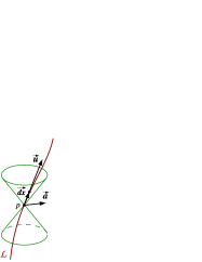
Figure 3: Worldline $\mathcal{L}$ of a particle, with the 4-velocity $\vec{\bm{u}}=c^{-1}d\vec{\bm{x}}/d\tau$ and the 4-acceleration $\vec{\bm{a}}$.

The 4-acceleration of the particle is the covariant derivative of the 4-velocity along itself:

$$\framebox{$\displaystyle\vec{\bm{a}}:=\bm{\nabla}_{\vec{\bm{u}}}\,\vec{\bm{u}}$}.$$ (36)

Since $\vec{\bm{u}}$ is a unit vector, it follows that

$$\vec{\bm{u}}\cdot\vec{\bm{a}}=0,$$ (37)

i.e. $\vec{\bm{a}}$ is orthogonal to $\vec{\bm{u}}$ with respect to the metric $\bm{g}$ (cf. Fig. 3). In particular, $\vec{\bm{a}}$ is a spacelike vector. Again, the 4-acceleration is not relative to any observer, but is intrinsic to the particle.

3.2 Observers, Lorentz factors and relative velocities

Let us consider an observer $\mathcal{O}_{0}$ (treated as a point mass particle) of worldline $\mathcal{L}_{0}$. Let us recall that, following Einstein’s convention for the definition of simultaneity, the set of events that are considered by $\mathcal{O}_{0}$ as being simultaneous to a given event $p$ on his worldline is a hypersurface of $\mathcal{M}$ which is orthogonal (with respect to $\bm{g}$) to $\mathcal{L}_{0}$ at $p$.

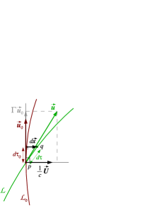
Figure 4: Relative velocity $\vec{\bm{U}}=d\vec{\bm{x}}/d\tau_{0}$ of a particle of 4-velocity $\vec{\bm{u}}$ with respect to an observer of 4-velocity $\vec{\bm{u}}_{0}$. $\vec{\bm{U}}$ enters in the orthogonal decomposition of $\vec{\bm{u}}$ with respect to $\vec{\bm{u}}_{0}$, via $\vec{\bm{u}}=\Gamma(\vec{\bm{u}}_{0}+c^{-1}\,\vec{\bm{U}})$. NB: contrary to what the figure might suggest, $d\tau_{0}>d\tau$.

Let $\mathcal{O}$ be another observer, whose worldline $\mathcal{L}$ intersects that of $\mathcal{O}_{0}$ at $p$. Let us denote by $\tau_{0}$ (resp. $\tau$) the proper time of $\mathcal{O}_{0}$ (resp. $\mathcal{O}$). After some infinitesimal proper time $d\tau$, $\mathcal{O}$ is located at the point $q$ (cf. Fig. 4). Let then $\tau_{0}+d\tau_{0}$ be the date attributed by $\mathcal{O}_{0}$ to the event $q$ according to the simultaneity convention recalled above. The relation between the proper time intervals $d\tau_{0}$ and $d\tau$ is

$$d\tau_{0}=\Gamma d\tau,$$ (38)

where $\Gamma$ is the Lorentz factor between the observers $\mathcal{O}_{0}$ and $\mathcal{O}$. We can express $\Gamma$ in terms of the 4-velocities $\vec{\bm{u}}_{0}$ and $\vec{\bm{u}}$ of $\mathcal{O}_{0}$ and $\mathcal{O}$. Indeed, let $d\vec{\bm{x}}$ the infinitesimal vector that is orthogonal to $\vec{\bm{u}}_{0}$ and links $\mathcal{L}_{0}$ to $q$ (cf. Fig. 4). Since $\vec{\bm{u}}_{0}$ and $\vec{\bm{u}}$ are unit vectors, the following equality holds:

$$c\,d\tau\vec{\bm{u}}=c\,d\tau_{0}\vec{\bm{u}}_{0}+d\vec{\bm{x}}.$$ (39)

Taking the scalar product with $\vec{\bm{u}}_{0}$, and using (38) as well as $\vec{\bm{u}}_{0}\cdot d\vec{\bm{x}}=0$ results in

$$\framebox{$\displaystyle\Gamma=-\vec{\bm{u}}_{0}\cdot\vec{\bm{u}}$}.$$ (40)

Hence from a geometrical point of view, the Lorentz factor is nothing but (minus) the scalar product of the unit vectors tangent to the two observers’ worldlines.

The velocity of $\mathcal{O}$ relative to $\mathcal{O}_{0}$ is simply the displacement vector $d\vec{\bm{x}}$ divided by the elapsed proper time of $\mathcal{O}_{0}$, $d\tau_{0}$:

$$\vec{\bm{U}}:=\frac{d\vec{\bm{x}}}{d\tau_{0}}.$$ (41)

$\vec{\bm{U}}$ is the “ordinary” velocity, by opposition to the 4-velocity $\vec{\bm{u}}$. Contrary to the latter, which is intrinsic to $\mathcal{O}$, $\vec{\bm{U}}$ depends upon the observer $\mathcal{O}_{0}$. Geometrically, $\vec{\bm{U}}$ can be viewed as the part of $\vec{\bm{u}}$ that is orthogonal to $\vec{\bm{u}}_{0}$, since by combining (38) and (39), we get

$$\framebox{$\displaystyle\vec{\bm{u}}=\Gamma\left(\vec{\bm{u}}_{0}+\frac{1}{c}\,\vec{\bm{U}}\right)$},\qquad\mbox{with}\quad\vec{\bm{u}}_{0}\cdot\vec{\bm{U}}=0.$$ (42)

Notice that Eq. (40) is a mere consequence of the above relation. The scalar square of Eq. (42), along with the normalization relations $\vec{\bm{u}}\cdot\vec{\bm{u}}=-1$ and $\vec{\bm{u}}_{0}\cdot\vec{\bm{u}}_{0}=-1$, leads to

$$\Gamma=\left(1-\frac{1}{c^{2}}\vec{\bm{U}}\cdot\vec{\bm{U}}\right)^{-1/2},$$ (43)

which is identical to the well-known expression from special relativity.

4 Fluid stress-energy tensor

4.1 General definition of the stress-energy tensor

The stress-energy tensor $\bm{T}$ is a tensor field on $\mathcal{M}$ which describes the matter content of spacetime, or more precisely the energy and momentum of matter, at a macroscopic level. $\bm{T}$ is a tensor field of type $(0,2)$ that is symmetric (this means that at each point $p\in\mathcal{M}$, $\bm{T}$ is a symmetric bilinear form on the vector space $\mathcal{T}_{p}(\mathcal{M})$) and that fulfills the following properties: given an observer $\mathcal{O}_{0}$ of 4-velocity $\vec{\bm{u}}_{0}$,

• the matter energy density as measured by $\mathcal{O}_{0}$ is

  $$E=\bm{T}(\vec{\bm{u}}_{0},\vec{\bm{u}}_{0});$$ (44)

• the matter momentum density as measured by $\mathcal{O}_{0}$ is

  $$\vec{\bm{p}}=-\frac{1}{c}\bm{T}(\vec{\bm{u}}_{0},\vec{\bm{e}}_{i})\,\vec{\bm{e}}_{i},$$ (45)

  where $(\vec{\bm{e}}_{i})$ is an orthonormal basis of the hyperplane orthogonal to $\mathcal{O}_{0}$’s worldline (rest frame of $\mathcal{O}_{0}$);

• the matter stress tensor as measured by $\mathcal{O}_{0}$ is

  $$S_{ij}=\bm{T}(\vec{\bm{e}}_{i},\vec{\bm{e}}_{j}),$$ (46)

  i.e. $\bm{T}(\vec{\bm{e}}_{i},\vec{\bm{e}}_{j})$ is the force in the direction $\vec{\bm{e}}_{i}$ acting on the unit surface whose normal is $\vec{\bm{e}}_{j}$.

4.2 Perfect fluid stress-energy tensor

The perfect fluid model of matter relies on a field of 4-velocities $\vec{\bm{u}}$, giving at each point the 4-velocity of a fluid particle. Moreover the perfect fluid is characterized by an isotropic pressure in the fluid frame (i.e. $S_{ij}=p\,\delta_{ij}$ for the observer whose 4-velocity is $\vec{\bm{u}}$). More precisely, the perfect fluid model is entirely defined by the following stress-energy tensor:

$$\framebox{$\displaystyle\bm{T}=(\rho c^{2}+p)\,\underline{\bm{u}}\otimes\underline{\bm{u}}+p\,\bm{g}$},$$ (47)

where $\rho$ and $p$ are two scalar fields, representing respectively the matter energy density (divided by $c^{2}$) and the pressure, both measured in the fluid frame, and $\underline{\bm{u}}$ is the 1-form associated to the 4-velocity $\vec{\bm{u}}$ by the metric tensor $\bm{g}$:

$$\begin{array}[]{cccl}\underline{\bm{u}}\ :&\mathcal{T}_{p}(\mathcal{M})&\longrightarrow&\mathbb{R}\\ &\vec{\bm{v}}&\longmapsto&\bm{g}(\vec{\bm{u}},\vec{\bm{v}})=\vec{\bm{u}}\cdot\vec{\bm{v}}.\end{array}$$ (48)

In terms of components with respect to a given basis $(\vec{\bm{e}}_{\alpha})$, if $\vec{\bm{u}}=u^{\alpha}\vec{\bm{e}}_{\alpha}$ and if $(\bm{e}^{\alpha})$ is the 1-form basis dual to $(\vec{\bm{e}}_{\alpha})$ (cf. Sec. 2.2), then $\underline{\bm{u}}=u_{\alpha}\bm{e}^{\alpha}$, with $u_{\alpha}=g_{\alpha\beta}u^{\beta}$. In Eq. (47), the tensor product $\underline{\bm{u}}\otimes\underline{\bm{u}}$ stands for the bilinear form $(\vec{\bm{v}},\vec{\bm{w}})\mapsto\langle\underline{\bm{u}},\vec{\bm{v}}\rangle\langle\underline{\bm{u}},\vec{\bm{w}}\rangle=(\vec{\bm{u}}\cdot\vec{\bm{v}})(\vec{\bm{u}}\cdot\vec{\bm{w}})$ [cf. (6)].

According to Eq. (44) the fluid energy density as measured by an observer $\mathcal{O}_{0}$ of 4-velocity $\vec{\bm{u}}_{0}$ is $E=\bm{T}(\vec{\bm{u}}_{0},\vec{\bm{u}}_{0})=(\rho c^{2}+p)(\vec{\bm{u}}\cdot\vec{\bm{u}}_{0})^{2}+p\bm{g}(\vec{\bm{u}}_{0},\vec{\bm{u}}_{0})$. Since $\vec{\bm{u}}\cdot\vec{\bm{u}}_{0}=-\Gamma$, where $\Gamma$ is the Lorentz factor between the fluid and $\mathcal{O}_{0}$ [Eq. (40)], and $\bm{g}(\vec{\bm{u}}_{0},\vec{\bm{u}}_{0})=-1$, we get

$$E=\Gamma^{2}(\rho c^{2}+p)-p.$$ (49)

The reader familiar with the formula $E=\Gamma mc^{2}$ may be puzzled by the $\Gamma^{2}$ factor in (49). However he should remind that $E$ is not an energy, but an energy per unit volume: the extra $\Gamma$ factor arises from “length contraction” in the direction of motion.

Similarly, by applying formula (45), we get the fluid momentum density as measured by the observer $\mathcal{O}_{0}$: $c\vec{\bm{p}}=-\bm{T}(\vec{\bm{u}}_{0},\vec{\bm{e}}_{i})\,\vec{\bm{e}}_{i}=-[(\rho c^{2}+p)(\vec{\bm{u}}\cdot\vec{\bm{u}}_{0})(\vec{\bm{u}}\cdot\vec{\bm{e}}_{i})+p\bm{g}(\vec{\bm{u}}_{0},\vec{\bm{e}}_{i})]\,\vec{\bm{e}}_{i}$, with $\vec{\bm{u}}\cdot\vec{\bm{u}}_{0}=-\Gamma$, $\bm{g}(\vec{\bm{u}}_{0},\vec{\bm{e}}_{i})=0$ and $(\vec{\bm{u}}\cdot\vec{\bm{e}}_{i})\,\vec{\bm{e}}_{i}$ being the projection of $\vec{\bm{u}}$ orthogonal to $\vec{\bm{u}}_{0}$: according to (42), $(\vec{\bm{u}}\cdot\vec{\bm{e}}_{i})\,\vec{\bm{e}}_{i}=\Gamma/c\,\vec{\bm{U}}$, where $\vec{\bm{U}}$ is the fluid velocity relative to $\mathcal{O}_{0}$. Hence

$$\vec{\bm{p}}=\Gamma^{2}\left(\rho+\frac{p}{c^{2}}\right)\vec{\bm{U}}.$$ (50)

Finally, by applying formula (46), we get the stress tensor as measured by the observer $\mathcal{O}_{0}$: $S_{ij}=\bm{T}(\vec{\bm{e}}_{i},\vec{\bm{e}}_{j})=(\rho c^{2}+p)(\vec{\bm{u}}\cdot\vec{\bm{e}}_{i})(\vec{\bm{u}}\cdot\vec{\bm{e}}_{j})+p\bm{g}(\vec{\bm{e}}_{i},\vec{\bm{e}}_{j})$, with $\vec{\bm{u}}\cdot\vec{\bm{e}}_{i}=\Gamma/c\,\vec{\bm{e}}_{i}\cdot\vec{\bm{U}}$ [thanks to Eq. (42) and $\vec{\bm{e}}_{i}\cdot\vec{\bm{u}}_{0}=0$] and $\bm{g}(\vec{\bm{e}}_{i},\vec{\bm{e}}_{j})=\delta_{ij}$. Hence

$$S_{ij}=p\,\delta_{ij}+\Gamma^{2}\left(\rho+\frac{p}{c^{2}}\right)U^{i}U^{j},$$ (51)

where $U^{i}$ is the $i$-th component of the velocity $\vec{\bm{U}}$ with respect to the orthonormal triad $(\vec{\bm{e}}_{i})$: $\vec{\bm{U}}=U^{i}\vec{\bm{e}}_{i}$.

Notice that if the observer $\mathcal{O}_{0}$ is comoving with the fluid, then $\vec{\bm{u}}_{0}=\vec{\bm{u}}$, $\Gamma=1$, $\vec{\bm{U}}=0$ and Eqs. (49), (50) and (51) reduce to

$$E=\rho c^{2},\quad\vec{\bm{p}}=0,\quad S_{ij}=p\,\delta_{ij}.$$ (52)

We thus recover the interpretation of the scalar fields $\rho$ and $p$ given above.

4.3 Concept of equation of state

Let us assume that at the microscopic level, the perfect fluid is constituted by $N$ species of particles ($N\geq 1$), so that the energy density $\rho c^{2}$ is a function of the number densities $n_{A}$ of particles of species $A$ ($A\in\{1,2,\ldots,N\}$) in the fluid rest frame (proper number density) and of the entropy density $s$ in the fluid rest frame:

$$\framebox{$\displaystyle\rho c^{2}=\varepsilon(s,n_{1},n_{2},\ldots,n_{N})$}.$$ (53)

The function $\varepsilon$ is called the equation of state (EOS) of the fluid. Notice that $\varepsilon$ is the total energy density, including the rest-mass energy: denoting by $m^{A}$ the individual mass of particles of species $A$, we may write

$$\varepsilon=\sum_{A}m^{A}n_{A}c^{2}+\varepsilon_{\rm int},$$ (54)

where $\varepsilon_{\rm int}$ is the “internal” energy density, containing the microscopic kinetic energy of the particles and the potential energy resulting from the interactions between the particles.

The first law of thermodynamics in a fixed small comobile volume $V$ writes

$$d\mathcal{E}=T\,dS+\sum_{A}\mu^{A}\,dN_{A},$$ (55)

where

• $\mathcal{E}$ is the total energy in volume $V$: $\mathcal{E}=\varepsilon V$,

• $S$ is the total entropy in $V$: $S=sV$,

• $N_{A}$ is the number of particles of species $A$ in $V$: $N_{A}=n_{A}V$,

• $T$ is the thermodynamical temperature,

• $\mu^{A}$ is the relativistic chemical potential of particles of particles of species $A$; it differs from the standard (non-relativistic) chemical potential ${\tilde{\mu}}^{A}$ by the mass $m^{A}$: $\mu^{A}={\tilde{\mu}}^{A}+m^{A}$, reflecting the fact that $\mathcal{E}$ includes the rest-mass energy.

Replacing $\mathcal{E}$, $S$ and $N_{A}$ by their expression in terms of $\varepsilon$, $s$, $n_{A}$ and $V$ leads to $d(\varepsilon V)=T\,d(sV)+\sum_{A}\mu^{A}\,d(n_{A}V)$. Since $V$ is held fixed, the first law of thermodynamics becomes

$$\framebox{$\displaystyle d\varepsilon=T\,ds+\sum_{A}\mu^{A}\,dn_{A}$}.$$ (56)

Consequently, $T$ and $\mu^{A}$ can be expressed as partial derivatives of the equation of state (53):

$$T=\left(\frac{\partial\varepsilon}{\partial s}\right)_{n_{A}}\qquad\mbox{and}\qquad\mu^{A}=\left(\frac{\partial\varepsilon}{\partial n_{A}}\right)_{s,n_{B\not=A}}.$$ (57)

Actually these relations can be taken as definitions for the temperature $T$ and chemical potential $\mu^{A}$. This then leads to the relation (56), which we will call hereafter the first law of thermodynamics.

5 Conservation of energy and momentum

5.1 General form

We shall take for the basis of our presentation of relativistic hydrodynamics the law of local conservation of energy and momentum of the fluid, which is assumed to be isolated:

$$\framebox{$\displaystyle\bm{\nabla}\cdot\bm{T}=0$}.$$ (58)

$\bm{\nabla}\cdot\bm{T}$ stands for the covariant divergence of the fluid stress-energy tensor $\bm{T}$. This is a 1-form, the components of which in a given basis are

$$(\bm{\nabla}\cdot\bm{T})_{\alpha}=\nabla^{\mu}T_{\mu\alpha}=g^{\mu\nu}\nabla_{\nu}T_{\mu\alpha}.$$ (59)

For a self-gravitating fluid, Eq. (58) is actually a consequence of the fundamental equation of general relativity, namely the Einstein equation. Indeed the latter relates the curvature associated with the metric $\bm{g}$ to the matter content of spacetime, according to

$$\bm{G}=\frac{8\pi G}{c^{4}}\bm{T},$$ (60)

where $\bm{G}$ is the so-called Einstein tensor, which represents some part of the Riemann curvature tensor of $(\mathcal{M},\bm{g})$. A basic property of the Einstein tensor is $\bm{\nabla}\cdot\bm{G}=0$ (this follows from the so-called Bianchi identities, which are pure geometric identities regarding the Riemann curvature tensor). Thus it is immediate that the Einstein equation (60) implies the energy-momentum conservation equation (58). Note that in this respect the situation is different from that of Newtonian theory, for which the gravitation law (Poisson equation) does not imply the conservation of energy and momentum of the matter source. We refer the reader to § 22.2 of (Hartle [2003]) for a more extended discussion of Eq. (58), in particular of the fact that it corresponds only to a local conservation of energy and momentum.

Let us mention that there exist formulations of relativistic hydrodynamics that do not use (58) as a starting point, but rather a variational principle. These Hamiltonian formulations have been pioneered by Taub ([1954]) and developed, among others, by Carter ([1973], [1979], [1989]), as well as Comer & Langlois ([1993]).

5.2 Application to a perfect fluid

Substituting the perfect fluid stress-energy tensor (47) in the energy-momentum conservation equation (58), and making use of (23) results in

$$\bm{\nabla}\cdot\bm{T}=0\ \iff\ \left[\bm{\nabla}_{\vec{\bm{u}}}(\varepsilon+p)+(\varepsilon+p)\bm{\nabla}\cdot\vec{\bm{u}}\right]\underline{\bm{u}}+(\varepsilon+p)\underline{\bm{a}}+\bm{\nabla}p=0,$$ (61)

where $\underline{\bm{a}}$ is the 1-form associated by the metric duality [cf. Eq. (48) with $\vec{\bm{u}}$ replaced by $\vec{\bm{a}}$] to the fluid 4-acceleration $\vec{\bm{a}}=\bm{\nabla}_{\vec{\bm{u}}}\,\vec{\bm{u}}$ [Eq. (36)]. The scalar $\bm{\nabla}\cdot\vec{\bm{u}}$ is the covariant divergence of the 4-velocity vector: it is the trace of the covariant derivative $\bm{\nabla}\vec{\bm{u}}$, the latter being a type $(1,1)$ tensor: $\bm{\nabla}\cdot\vec{\bm{u}}=\nabla_{\sigma}u^{\sigma}$. Notice that $\bm{\nabla}p$ in Eq. (61) is nothing but the gradient of the pressure field: $\bm{\nabla}p=\bm{\mathrm{d}}p$ (cf. item (i) in Sec. 2.4.2).

5.3 Projection along $\vec{\bm{u}}$

Equation (61) is an identity involving 1-forms. If we apply it to the vector $\vec{\bm{u}}$, we get a scalar field. Taking into account $\langle\underline{\bm{u}},\vec{\bm{u}}\rangle=\vec{\bm{u}}\cdot\vec{\bm{u}}=-1$ and $\langle\underline{\bm{a}},\vec{\bm{u}}\rangle=\vec{\bm{a}}\cdot\vec{\bm{u}}=0$ [Eq. (37)], the scalar equation becomes

$$\langle\bm{\nabla}\cdot\bm{T},\vec{\bm{u}}\rangle=0\ \iff\ \bm{\nabla}_{\vec{\bm{u}}}\,\varepsilon=-(\varepsilon+p)\bm{\nabla}\cdot\vec{\bm{u}}.$$ (62)

Notice that $\bm{\nabla}_{\vec{\bm{u}}}\,\varepsilon=\langle\bm{\mathrm{d}}\varepsilon,\vec{\bm{u}}\rangle=\bm{\mathcal{L}}_{\vec{\bm{u}}}\,\varepsilon$ (cf. item (i) at the end of Sec. 2.4.1). Now, the first law of thermodynamics (56) yields

$$\bm{\nabla}_{\vec{\bm{u}}}\,\varepsilon=T\bm{\nabla}_{\vec{\bm{u}}}\,s+\sum_{A}\mu^{A}\bm{\nabla}_{\vec{\bm{u}}}\,n_{A},$$ (63)

so that Eq. (62) can be written as

$$\langle\bm{\nabla}\cdot\bm{T},\vec{\bm{u}}\rangle=0 \iff T\bm{\nabla}\cdot(s\vec{\bm{u}})+\sum_{A}\mu^{A}\bm{\nabla}\cdot(n_{A}\vec{\bm{u}})$$ (64)

$$\ \quad+\left(\varepsilon+p-Ts-\sum_{A}\mu^{A}n_{A}\right)\bm{\nabla}\cdot\vec{\bm{u}}=0.$$

Now, we recognize in $\mathcal{G}:=\varepsilon+p-Ts$ the free enthalpy (also called Gibbs free energy) per unit volume. It is well known that the free enthalpy $G=\mathcal{G}V=E+PV-TS$ (where $V$ is some small volume element) obeys the thermodynamic identity

$$G=\sum_{A}\mu^{A}N_{A},$$ (65)

from which we get $\mathcal{G}=\sum_{A}\mu^{A}n_{A}$, i.e.

$$\framebox{$\displaystyle p=Ts+\sum_{A}\mu^{A}n_{A}-\varepsilon$}.$$ (66)

This relation shows that $p$ is a function of $(s,n_{1},\ldots,n_{N})$ which is fully determined by $\varepsilon(s,n_{1},\ldots,n_{N})$ [recall that $T$ and $\mu^{A}$ are nothing but partial derivatives of the latter, Eq. (57)]. Another way to get the identity (66) is to start from the first law of thermodynamics in the form (55), but allowing for the volume $V$ to vary, i.e. adding the term $-p\,dV$ to it:

$$d\mathcal{E}=T\,dS-p\,dV+\sum_{A}\mu^{A}\,dN_{A}.$$ (67)

Substituting $\mathcal{E}=\varepsilon V$, $S=sV$ and $N_{A}=n_{A}V$ is this formula and using (56) leads to (66).

For our purpose the major consequence of the thermodynamic identity (66) is that Eq. (64) simplifies substantially:

$$\langle\bm{\nabla}\cdot\bm{T},\vec{\bm{u}}\rangle=0\ \iff\ \framebox{$\displaystyle T\bm{\nabla}\cdot(s\vec{\bm{u}})+\sum_{A}\mu^{A}\bm{\nabla}\cdot(n_{A}\vec{\bm{u}})=0$}.$$ (68)

In this equation, $c\bm{\nabla}\cdot(s\vec{\bm{u}})$ is the entropy creation rate (entropy created per unit volume and unit time in the fluid frame) and $c\bm{\nabla}\cdot(n_{A}\vec{\bm{u}})$ is the particle creation rate of species $A$ (number of particles created par unit volume and unit time in the fluid frame). This follows from

$$c\bm{\nabla}\cdot(n_{A}\vec{\bm{u}})=c(\bm{\nabla}_{\vec{\bm{u}}}n_{A}+n_{A}\bm{\nabla}\cdot\vec{\bm{u}})=\frac{dn_{A}}{d\tau}+n_{A}\frac{1}{V}\frac{dV}{d\tau}=\frac{1}{V}\frac{d(n_{A}V)}{d\tau},$$ (69)

where $\tau$ is the fluid proper time and where we have used the expansion rate formula

$$\bm{\nabla}\cdot\vec{\bm{u}}=\frac{1}{cV}\frac{dV}{d\tau},$$ (70)

$V$ being a small volume element dragged along by $\vec{\bm{u}}$. Equation (68) means that in a perfect fluid, the only process that may increase the entropy is the creation of particles.

5.4 Projection orthogonally to $\vec{\bm{u}}$: relativistic Euler equation

Let us now consider the projection of (61) orthogonally to the 4-velocity. The projector orthogonal to $\vec{\bm{u}}$ is the operator $\bm{P}:=\bm{1}+\vec{\bm{u}}\otimes\underline{\bm{u}}$:

$$\begin{array}[]{cccl}\bm{P}\ :&\mathcal{T}_{p}(\mathcal{M})&\longrightarrow&\mathcal{T}_{p}(\mathcal{M})\\ &\vec{\bm{v}}&\longmapsto&\vec{\bm{v}}+(\vec{\bm{u}}\cdot\vec{\bm{v}})\vec{\bm{u}}.\end{array}$$ (71)

Combining $\bm{P}$ to the 1-form (61), and using $\underline{\bm{u}}\circ\bm{P}=0$ as well as $\underline{\bm{a}}\circ\bm{P}=\underline{\bm{a}}$, leads to the 1-form equation

$$(\bm{\nabla}\cdot\bm{T})\circ\bm{P}=0\ \iff\ \framebox{$\displaystyle(\varepsilon+p)\underline{\bm{a}}=-\bm{\nabla}p-(\bm{\nabla}_{\vec{\bm{u}}}\,p)\underline{\bm{u}}$}.$$ (72)

This is clearly an equation of the type “ $m\vec{a}=\vec{F}$ ”, although the gravitational “force” is hidden in the covariant derivative in the derivation of $\vec{\bm{a}}$ from $\vec{\bm{u}}$. We may consider that (72) is a relativistic version of the classical Euler equation.

Most textbooks stop at this point, considering that (72) is a nice equation. However, as stated in the Introduction, there exists an alternative form for the equation of motion of a perfect fluid, which turns out to be much more useful than (72), especially regarding the derivation of conservation laws: it is the Carter-Lichnerowicz form, to which the rest of this lecture is devoted.

6 Carter-Lichnerowicz equation of motion

6.1 Derivation

In the right hand-side of the relativistic Euler equation (72) appears the gradient of the pressure field: $\bm{\nabla}p=\bm{\mathrm{d}}p$. Now, by deriving the thermodynamic identity (66) and combining with the first law (56), we get the relation

$$\framebox{$\displaystyle dp=s\,dT+\sum_{A}n_{A}d\mu^{A}$},$$ (73)

which is known as the Gibbs-Duhem relation. We may use this relation to express $\bm{\nabla}p$ in terms of $\bm{\nabla}T$ and $\bm{\nabla}\mu^{A}$ in Eq. (72). Also, by making use of (66), we may replace $\varepsilon+p$ by $Ts+\sum_{A}\mu^{A}n_{A}$. Hence Eq. (72) becomes

$$\left(Ts+\sum_{A}\mu^{A}n_{A}\right)\underline{\bm{a}}=-s\bm{\nabla}T-\sum_{A}n_{A}\bm{\nabla}\mu^{A}-\left(s\bm{\nabla}_{\vec{\bm{u}}}\,T+\sum_{A}n_{A}\bm{\nabla}_{\vec{\bm{u}}}\,\mu^{A}\right)\underline{\bm{u}}.$$ (74)

Writing $\underline{\bm{a}}=\vec{\bm{\nabla}}_{\vec{\bm{u}}}\underline{\bm{u}}$ and reorganizing slightly yields

$$s\left[\bm{\nabla}_{\vec{\bm{u}}}(T\underline{\bm{u}})+\bm{\nabla}T\right]+\sum_{A}n_{A}\left[\bm{\nabla}_{\vec{\bm{u}}}(\mu^{A}\underline{\bm{u}})+\bm{\nabla}\mu^{A}\right]=0.$$ (75)

The next step amounts to noticing that

$$\bm{\nabla}_{\vec{\bm{u}}}(T\underline{\bm{u}})=\bm{\mathcal{L}}_{\vec{\bm{u}}}\,(T\underline{\bm{u}}).$$ (76)

This is easy to establish, starting from expression (16) for the Lie derivative of a 1-form, in which we may replace the partial derivatives by covariant derivatives [thanks to the symmetry of the Christoffel symbols, cf. Eq. (21)]:

$${\mathcal{L}}_{\vec{\bm{u}}}\,(Tu_{\alpha})=u^{\mu}\nabla_{\mu}(Tu_{\alpha})+Tu_{\mu}\nabla_{\alpha}u^{\mu},$$ (77)

i.e.

$$\bm{\mathcal{L}}_{\vec{\bm{u}}}\,(T\underline{\bm{u}})=\bm{\nabla}_{\vec{\bm{u}}}(T\underline{\bm{u}})+T\,\vec{\bm{u}}\cdot\bm{\nabla}\vec{\bm{u}}.$$ (78)

Now, from $\vec{\bm{u}}\cdot\vec{\bm{u}}=-1$, we get $\vec{\bm{u}}\cdot\bm{\nabla}\vec{\bm{u}}=0$, which establishes (76).

On the other side, the Cartan identity (32) yields

$$\bm{\mathcal{L}}_{\vec{\bm{u}}}\,(T\underline{\bm{u}})=\vec{\bm{u}}\cdot\bm{\mathrm{d}}(T\underline{\bm{u}})+\bm{\mathrm{d}}[T\underbrace{\langle\underline{\bm{u}},\vec{\bm{u}}\rangle}_{=-1}]=\vec{\bm{u}}\cdot\bm{\mathrm{d}}(T\underline{\bm{u}})-\bm{\mathrm{d}}T.$$ (79)

Combining this relation with (76) (noticing that $\bm{\mathrm{d}}T=\bm{\nabla}T$), we get

$$\bm{\nabla}_{\vec{\bm{u}}}(T\underline{\bm{u}})+\bm{\nabla}T=\vec{\bm{u}}\cdot\bm{\mathrm{d}}(T\underline{\bm{u}}).$$ (80)

Similarly,

$$\bm{\nabla}_{\vec{\bm{u}}}(\mu^{A}\underline{\bm{u}})+\bm{\nabla}\mu^{A}=\vec{\bm{u}}\cdot\bm{\mathrm{d}}(\mu^{A}\underline{\bm{u}}).$$ (81)

According to the above two relations, the equation of motion (75) can be re-written as

$$s\,\vec{\bm{u}}\cdot\bm{\mathrm{d}}(T\underline{\bm{u}})+\sum_{A}n_{A}\,\vec{\bm{u}}\cdot\bm{\mathrm{d}}(\mu^{A}\underline{\bm{u}})=0.$$ (82)

In this equation, appears the 1-form

$$\framebox{$\displaystyle\bm{\pi}^{A}:=\mu^{A}\underline{\bm{u}}$},$$ (83)

which is called the momentum 1-form of particles of species $A$. It is called momentum because in the Hamiltonian formulations mentioned in Sec. 5.1, this 1-form is the conjugate of the number density current $n_{A}\vec{\bm{u}}$.

Actually, it is the exterior derivative of $\bm{\pi}^{A}$ which appears in Eq. (82):

$$\framebox{$\displaystyle\bm{w}^{A}:=\bm{\mathrm{d}}\bm{\pi}^{A}$}.$$ (84)

This 2-form is called the vorticity 2-form of particles of species $A$. With this definition, Eq. (82) becomes

$$\framebox{$\displaystyle\sum_{A}n_{A}\,\vec{\bm{u}}\cdot\bm{w}^{A}+s\,\vec{\bm{u}}\cdot\bm{\mathrm{d}}(T\underline{\bm{u}})=0$}.$$ (85)

This is the Carter-Lichnerowicz form of the equation of motion for a multi-constituent perfect fluid. It has been considered by Lichnerowicz ([1967]) in the case of a single-constituent fluid ($N=1$) and generalized by Carter ([1979], [1989]) to the multi-constituent case. Let us stress that this is an equation between 1-forms. For instance $\vec{\bm{u}}\cdot\bm{w}^{A}$ is the 1-form $\bm{w}^{A}(\vec{\bm{u}},.)$, i.e. at each point $p\in\mathcal{M}$, this is the linear application $\mathcal{T}_{p}\rightarrow\mathbb{R}$, $\vec{\bm{v}}\mapsto\bm{w}^{A}(\vec{\bm{u}},\vec{\bm{v}})$. Since $\bm{w}^{A}$ is antisymmetric (being a 2-form), $\bm{w}^{A}(\vec{\bm{u}},\vec{\bm{u}})=0$. Hence the Carter-Lichnerowicz equation (85) is clearly a non-trivial equation only in the three dimensions orthogonal to $\vec{\bm{u}}$.

6.2 Canonical form for a simple fluid

Let us define a simple fluid as a fluid for which the EOS (53) takes the form

$$\framebox{$\displaystyle\varepsilon=\varepsilon(s,n)$},$$ (86)

where $n$ is the baryon number density in the fluid rest frame. The simple fluid model is valid in two extreme cases:

• when the reaction rates between the various particle species are very low: the composition of matter is then frozen: all the particle number densities can be deduced from the baryon number: $n_{A}=Y_{A}n$, with a fixed species fraction $Y_{A}$;

• when reaction rates between the various particle species are very high, ensuring a complete chemical (nuclear) equilibrium. In this case, all the $n_{A}$ are uniquely determined by $n$ and $s$, via $n_{A}=Y_{A}^{\rm eq}(s,n)\,n$.

A special case of a simple fluid is that of barotropic fluid, for which

$$\varepsilon=\varepsilon(n).$$ (87)

This subcase is particularly relevant for cold dense matter, as in white dwarfs and neutron stars.

Thanks to Eq. (86), a simple fluid behaves as if it contains a single particle species: the baryons. All the equations derived previously apply, setting $N=1$ (one species) and $A=1$.

Since $n$ is the baryon number density, it must obey the fundamental law of baryon conservation:

$$\framebox{$\displaystyle\bm{\nabla}\cdot(n\vec{\bm{u}})=0$}.$$ (88)

That this equation does express the conservation of baryon number should be obvious after the discussion in Sec. 5.3, from which it follows that $c\bm{\nabla}\cdot(n\vec{\bm{u}})$ is the number of baryons created per unit volume and unit time in a comoving fluid element.

The projection of $\bm{\nabla}\cdot\bm{T}=0$ along $\vec{\bm{u}}$, Eq. (68) then implies

$$\framebox{$\displaystyle\bm{\nabla}\cdot(s\vec{\bm{u}})=0$}.$$ (89)

This means that the evolution of a (isolated) simple fluid is necessarily adiabatic.

On the other side, the Carter-Lichnerowicz equation (85) reduces to

$$n\,\vec{\bm{u}}\cdot\bm{w}^{\rm b}+s\,\vec{\bm{u}}\cdot\bm{\mathrm{d}}(T\underline{\bm{u}})=0,$$ (90)

where we have used the label ${\rm b}$ (for baryon) instead of the running letter $A$: $\bm{w}^{\rm b}=\bm{\mathrm{d}}(\mu\underline{\bm{u}})$ [Eqs. (83) and (84)], $\mu$ being the chemical potentials of baryons:

$$\mu:=\left(\frac{\partial\varepsilon}{\partial n}\right)_{s}.$$ (91)

Let us rewrite Eq. (90) as

$$\vec{\bm{u}}\cdot\left[\bm{\mathrm{d}}(\mu\underline{\bm{u}})+{\bar{s}}\,\bm{\mathrm{d}}(T\underline{\bm{u}})\right]=0,$$ (92)

where we have introduced the entropy per baryon:

$$\framebox{$\displaystyle\bar{s}:=\frac{s}{n}$}.$$ (93)

In view of Eq. (92), let us define the fluid momentum per baryon 1-form by

$$\bm{\pi}:=(\mu+T{\bar{s}})\underline{\bm{u}}$$ (94)

and the fluid vorticity 2-form as its exterior derivative:

$$\framebox{$\displaystyle\bm{w}:=\bm{\mathrm{d}}\bm{\pi}$}.$$ (95)

Notice that $\bm{w}$ is not equal to the baryon vorticity: $\bm{w}=\bm{w}^{\rm b}+\bm{\mathrm{d}}({\bar{s}}T\underline{\bm{u}})$. Since in the present case the thermodynamic identity (66) reduces to $p=Ts+\mu n-\varepsilon$, we have

$$\framebox{$\displaystyle\mu+T{\bar{s}}=\frac{\varepsilon+p}{n}=:h$},$$ (96)

where $h$ is the enthalpy per baryon. Accordingly the fluid momentum per baryon 1-form is simply

$$\framebox{$\displaystyle\bm{\pi}=h\,\underline{\bm{u}}$}.$$ (97)

By means of formula (27), we can expand the exterior derivative $\bm{\mathrm{d}}({\bar{s}}T\underline{\bm{u}})$ as

$$\bm{\mathrm{d}}({\bar{s}}T\underline{\bm{u}})=\bm{\mathrm{d}}{\bar{s}}\wedge(T\underline{\bm{u}})+{\bar{s}}\,\bm{\mathrm{d}}(T\underline{\bm{u}})=T\bm{\mathrm{d}}{\bar{s}}\wedge\underline{\bm{u}}+{\bar{s}}\,\bm{\mathrm{d}}(T\underline{\bm{u}}),$$ (98)

where the symbol $\wedge$ stands for the exterior product: for any pair $(\bm{a},\bm{b})$ of 1-forms, $\bm{a}\wedge\bm{b}$ is the 2-form defined as $\bm{a}\wedge\bm{b}=\bm{a}\otimes\bm{b}-\bm{b}\otimes\bm{a}$. Thanks to (98), the fluid vorticity 2-form, given by Eqs. (95) and (94), can be written as

$$\bm{w}=\bm{\mathrm{d}}(\mu\underline{\bm{u}})+{\bar{s}}\,\bm{\mathrm{d}}(T\underline{\bm{u}})+T\bm{\mathrm{d}}{\bar{s}}\wedge\underline{\bm{u}}.$$ (99)

Therefore, we may rewrite (92) by letting appear $\bm{w}$, to get successively

$$\vec{\bm{u}}\cdot(\bm{w}-T\bm{\mathrm{d}}{\bar{s}}\wedge\underline{\bm{u}})=0,$$

$$\vec{\bm{u}}\cdot\bm{w}-T\vec{\bm{u}}\cdot(\bm{\mathrm{d}}{\bar{s}}\wedge\underline{\bm{u}})=0,$$

$$\vec{\bm{u}}\cdot\bm{w}-T\left[\langle\bm{\mathrm{d}}{\bar{s}},\vec{\bm{u}}\rangle\,\underline{\bm{u}}-\langle\underline{\bm{u}},\vec{\bm{u}}\rangle\bm{\mathrm{d}}{\bar{s}}\right]=0,$$

$$\vec{\bm{u}}\cdot\bm{w}-T\left[(\bm{\nabla}_{\vec{\bm{u}}}\,{\bar{s}})\,\underline{\bm{u}}+\bm{\mathrm{d}}{\bar{s}}\right]=0.$$ (100)

Now from the baryon number and entropy conservation equations (88) and (89), we get

$$\framebox{$\displaystyle\bm{\nabla}_{\vec{\bm{u}}}\,{\bar{s}}=0$},$$ (101)

i.e. the entropy per baryon is conserved along the fluid lines. Reporting this property in Eq. (100) leads to the equation of motion

$$\framebox{$\displaystyle\framebox{$\displaystyle\vec{\bm{u}}\cdot\bm{w}=T\bm{\mathrm{d}}{\bar{s}}$}$}.$$ (102)

This equation was first obtained by Lichnerowicz ([1967]). In the equivalent form (assuming $T\not=0$),

$$\vec{\bm{u}}^{\prime}\cdot\bm{w}=\bm{\mathrm{d}}{\bar{s}},\qquad\mbox{with}\quad\vec{\bm{u}}^{\prime}:=\frac{1}{T}\vec{\bm{u}},$$ (103)

it has been called a canonical equation of motion by Carter ([1979]), who has shown that it can be derived from a variational principle.

Owing to its importance, let us make (102) explicit in terms of components [cf. (26) and (27)]:

$$u^{\mu}\left[\frac{\partial}{\partial x^{\mu}}(h\,u_{\alpha})-\frac{\partial}{\partial x^{\alpha}}(h\,u_{\mu})\right]=T\frac{\partial{\bar{s}}}{\partial x^{\alpha}}.$$ (104)

6.3 Isentropic case (barotropic fluid)

For an isentropic fluid, ${\bar{s}}={\rm const}$. The EOS is then barotropic, i.e. it can be cast in the form (87). For this reason, the isentropic simple fluid is also called a single-constituent fluid. In this case, the gradient $\bm{\mathrm{d}}{\bar{s}}$ vanishes and the Carter-Lichnerowicz equation of motion (102) reduces to

$$\framebox{$\displaystyle\vec{\bm{u}}\cdot\bm{w}=0$}.$$ (105)

This equation has been first exhibited by Synge ([1937]). Its simplicity is remarkable, especially if we compare it to the equivalent Euler form (72). Indeed it should be noticed that the assumption of a single-constituent fluid leaves the relativistic Euler equation as it is written in (72), whereas it leads to the simple form (105) for the Carter-Lichnerowicz equation of motion.

In the isentropic case, there is a useful relation between the gradient of pressure and that of the enthalpy per baryon. Indeed, from Eq. (96), we have $d\varepsilon+dp=d(nh)=n\,dh+h\,dn$. Substituting Eq. (56) for $d\varepsilon$ yields $T\,ds+\mu\,dn+dp=n\,dh+h\,dn$. But $T\,ds=T\,d(n{\bar{s}})=T{\bar{s}}\,dn$ since $d{\bar{s}}=0$. Using Eq. (96) again then leads to

$$dp=n\,dh,$$ (106)

or equivalently,

$$\frac{dp}{\varepsilon+p}=d\ln h.$$ (107)

If we come back to the relativistic Euler equation (72), the above relation shows that in the isentropic case, it can be written as the fluid 4-acceleration being the orthogonal projection (with respect to $\vec{\bm{u}}$) of a pure gradient (that of $-\ln h$):

$$\underline{\bm{a}}=-\bm{\mathrm{d}}\ln h-\langle\bm{\mathrm{d}}\ln h,\vec{\bm{u}}\rangle\,\underline{\bm{u}}.$$ (108)

6.4 Newtonian limit: Crocco equation

Let us go back to the non isentropic case and consider the Newtonian limit of the Carter-Lichnerowicz equation (102). For this purpose let us assume that the gravitational field is weak and static. It is then always possible to find a coordinate system $(x^{\alpha})=(x^{0}=ct,x^{i})$ such that the metric components take the form

$$g_{\alpha\beta}dx^{\alpha}dx^{\beta}=-\left(1+2\frac{\Phi}{c^{2}}\right)\,c^{2}dt^{2}+\left(1-2\frac{\Phi}{c^{2}}\right)f_{ij}dx^{i}dx^{j},$$ (109)

where $\Phi$ is the Newtonian gravitational potential (solution of $\Delta\Phi=4\pi G\rho$) and $f_{ij}$ is the flat metric in the usual 3-dimensional Euclidean space. For a weak gravitational field (Newtonian limit), $|\Phi|/c^{2}\ll 1$. The components of the fluid 4-velocity are deduced from Eq. (34): $u^{\alpha}=c^{-1}dx^{\alpha}/d\tau$, $\tau$ being the fluid proper time. Thus (recall that $x^{0}=ct$)

$$u^{\alpha}=\left(u^{0},u^{0}\frac{v^{i}}{c}\right),\quad\mbox{with}\quad u^{0}=\frac{dt}{d\tau}\quad\mbox{and}\quad v^{i}:=\frac{dx^{i}}{dt}.$$ (110)

At the Newtonian limit, the $v^{i}$’s are of course the components of the fluid velocity $\vec{v}$ with respect to the inertial frame defined by the coordinates $(x^{\alpha})$. That the coordinates $(x^{\alpha})$ are inertial in the Newtonian limit is obvious from the form (109) of the metric, which is clearly Minkowskian when $\Phi\rightarrow 0$. Consistent with the Newtonian limit, we assume that $|\vec{v}|/c\ll 1$. The normalization relation $g_{\alpha\beta}u^{\alpha}u^{\beta}=-1$ along with (110) enables us to express $u^{0}$ in terms of $\Phi$ and $\vec{v}$. To the first order in $\Phi/c^{2}$ and $\vec{v}\cdot\vec{v}/c^{2}=v_{j}v^{j}/c^{2}$ (), we get

$$u^{0}\simeq 1-\frac{\Phi}{c^{2}}+\frac{v_{j}v^{j}}{2c^{2}}.$$ (111)

To that order of approximation, we may set $u^{0}\simeq 1$ in the spatial part of $u^{\alpha}$ and rewrite (110) as

$$u^{\alpha}\simeq\left(u^{0},\frac{v^{i}}{c}\right)\simeq\left(1-\frac{\Phi}{c^{2}}+\frac{v_{j}v^{j}}{2c^{2}},\ \frac{v^{i}}{c}\right).$$ (112)

The components of $\underline{\bm{u}}$ are obtained from $u_{\alpha}=g_{\alpha\beta}u^{\beta}$, with $g_{\alpha\beta}$ given by (109). One gets

$$u_{\alpha}\simeq\left(u_{0},\frac{v_{i}}{c}\right)\simeq\left(-1-\frac{\Phi}{c^{2}}-\frac{v_{j}v^{j}}{2c^{2}},\ \frac{v_{i}}{c}\right).$$ (113)

To form the fluid vorticity $\bm{w}$ we need the enthalpy per baryon $h$. By combining Eq. (96) with Eq. (54) written as $\varepsilon=m_{\rm b}nc^{2}+\varepsilon_{\rm int}$ (where $m_{\rm b}$ is the mean mass of one baryon: $m_{\rm b}\simeq 1.66\times 10^{-27}{\rm\ kg}$), we get

$$h=m_{\rm b}c^{2}\left(1+\frac{H}{c^{2}}\right),$$ (114)

where $H$ is the non-relativistic (i.e. excluding the rest-mass energy) specific enthalpy (i.e. enthalpy per unit mass):

$$H:=\frac{\varepsilon_{\rm int}+p}{m_{\rm b}n}.$$ (115)

From (104), we have, for $i\in\{1,2,3\}$,

$$u^{\mu}w_{\mu i} = u^{\mu}\left[\frac{\partial}{\partial x^{\mu}}(h\,u_{i})-\frac{\partial}{\partial x^{i}}(h\,u_{\mu})\right]$$ (116)

$$= u^{0}\left[\frac{1}{c}\frac{\partial}{\partial t}(h\,u_{i})-\frac{\partial}{\partial x^{i}}(h\,u_{0})\right]+u^{j}\left[\frac{\partial}{\partial x^{j}}(h\,u_{i})-\frac{\partial}{\partial x^{i}}(h\,u_{j})\right].$$

Plugging Eqs. (112), (113) and (114) yields

$$\frac{u^{\mu}w_{\mu i}}{m_{\rm b}} = u^{0}\left\{\frac{\partial}{\partial t}\left[\left(1+\frac{H}{c^{2}}\right)v_{i}\right]-\frac{\partial}{\partial x^{i}}\left[(c^{2}+H)u_{0}\right]\right\}$$ (117)

$$+v^{j}\left\{\frac{\partial}{\partial x^{j}}\left[\left(1+\frac{H}{c^{2}}\right)v_{i}\right]-\frac{\partial}{\partial x^{i}}\left[\left(1+\frac{H}{c^{2}}\right)v_{j}\right]\right\}.$$

At the Newtonian limit, the terms $u^{0}$ and $H/c^{2}$ in the above equation can be set to respectively $1$ and $0$. Moreover, thanks to (113),

$$\frac{\partial}{\partial x^{i}}\left[(c^{2}+H)u_{0}\right] = -\frac{\partial}{\partial x^{i}}\left[(c^{2}+H)\left(1+\frac{\Phi}{c^{2}}+\frac{v_{j}v^{j}}{2c^{2}}\right)\right]$$ (118)

$$\simeq -\frac{\partial}{\partial x^{i}}\left(\Phi+\frac{1}{2}v_{j}v^{j}+H\right).$$

Finally we get

$$\frac{u^{\mu}w_{\mu i}}{m_{\rm b}}=\frac{\partial v_{i}}{\partial t}+\frac{\partial}{\partial x^{i}}\left(H+\frac{1}{2}v_{j}v^{j}+\Phi\right)+v^{j}\left(\frac{\partial v_{i}}{\partial x^{j}}-\frac{\partial v_{j}}{\partial x^{i}}\right).$$ (119)

The last term can be expressed in terms of the cross product between $\vec{v}$ and its the (3-dimensional) curl:

$$v^{j}\left(\frac{\partial v_{i}}{\partial x^{j}}-\frac{\partial v_{j}}{\partial x^{i}}\right)=-\left(\vec{v}\times\mathrm{curl}\,\vec{v}\right)_{i}.$$ (120)

In view of (119) and (120), we conclude that the Newtonian limit of the Carter-Lichnerowicz canonical equation (102) is

$$\frac{\partial v_{i}}{\partial t}+\frac{\partial}{\partial x^{i}}\left(H+\frac{1}{2}v_{j}v^{j}+\Phi\right)-\left(\vec{v}\times\mathrm{curl}\,\vec{v}\right)_{i}=T\frac{\partial{\tilde{s}}}{\partial x^{i}},$$ (121)

where ${\tilde{s}}:={\bar{s}}/m_{\rm b}$ is the specific entropy (i.e. entropy per unit mass). Equation (121) is known as the Crocco equation [see e.g. (Rieutord [1997])]. It is of course an alternative form of the classical Euler equation in the gravitational potential $\Phi$.

7 Conservation theorems

In this section, we illustrate the power of the Carter-Lichnerowicz equation by deriving from it various conservation laws in a very easy way. We consider a simple fluid, i.e. the EOS depends only on the baryon number density and the entropy density [Eq. (86)].

7.1 Relativistic Bernoulli theorem

7.1.1 Conserved quantity associated with a spacetime symmetry

Let us suppose that the spacetime $(\mathcal{M},\bm{g})$ has some symmetry described by the invariance under the action of a one-parameter group $\mathcal{G}$: for instance $\mathcal{G}=(\mathbb{R},+)$ for stationarity (invariance by translation along timelike curves) or $\mathcal{G}=\mathrm{SO(2)}$ for axisymmetry (invariance by rotation around some axis). Then one can associate to $\mathcal{G}$ a vector field $\vec{\bm{\xi}}$ such that an infinitesimal transformation of parameter $\epsilon$ in the group $\mathcal{G}$ corresponds to the infinitesimal displacement $\epsilon\vec{\bm{\xi}}$. In particular the field lines of $\vec{\bm{\xi}}$ are the trajectories (also called orbits) of $\mathcal{G}$. $\vec{\bm{\xi}}$ is called a generator of the symmetry group $\mathcal{G}$ or a Killing vector of spacetime. That the metric tensor $\bm{g}$ remains invariant under $\mathcal{G}$ is then expressed by the vanishing of the Lie derivative of $\bm{g}$ along $\vec{\bm{\xi}}$:

$$\framebox{$\displaystyle\bm{\mathcal{L}}_{\vec{\bm{\xi}}}\,\bm{g}=0$}.$$ (122)

Expressing the Lie derivative via Eq. (15) with the partial derivatives replaced by covariant ones [cf. remark below Eq. (76)], we immediately get that (122) is equivalent to the following requirement on the 1-form $\underline{\bm{\xi}}$ associated to $\vec{\bm{\xi}}$ by the metric duality:

$$\nabla_{\alpha}\xi_{\beta}+\nabla_{\beta}\xi_{\alpha}=0.$$ (123)

Equation (123) is called the Killing equation. It fully characterizes Killing vectors in a given spacetime.

The invariance of the fluid under the symmetry group $\mathcal{G}$ amounts to the vanishing of the Lie derivative along $\vec{\bm{\xi}}$ of all the tensor fields associated with matter. In particular, for the fluid momentum per baryon 1-form $\bm{\pi}$ introduced in Sec. 6.2:

$$\bm{\mathcal{L}}_{\vec{\bm{\xi}}}\,\bm{\pi}=0.$$ (124)

By means of the Cartan identity (32), this equation is recast as

$$\vec{\bm{\xi}}\cdot\bm{w}+\bm{\mathrm{d}}\langle\bm{\pi},\vec{\bm{\xi}}\rangle=0,$$ (125)

where we have replaced the exterior derivative $\bm{\mathrm{d}}\bm{\pi}$ by the vorticity 2-form $\bm{w}$ [cf. Eq. (95)] and we have written $\vec{\bm{\xi}}\cdot\bm{\pi}=\langle\bm{\pi},\vec{\bm{\xi}}\rangle$ (scalar field resulting from the action of the 1-form $\bm{\pi}$ on the vector $\vec{\bm{\xi}}$). The left-hand side of Eq. (125) is a 1-form. Let us apply it to the vector $\vec{\bm{u}}$:

$$\bm{w}(\vec{\bm{\xi}},\vec{\bm{u}})+\bm{\nabla}_{\vec{\bm{u}}}\langle\bm{\pi},\vec{\bm{\xi}}\rangle=0$$ (126)

Now, since $\bm{w}$ is antisymmetric, $\bm{w}(\vec{\bm{\xi}},\vec{\bm{u}})=-\bm{w}(\vec{\bm{u}},\vec{\bm{\xi}})$ and we may use the Carter-Lichnerowicz equation of motion (102) which involves $\bm{w}(\vec{\bm{u}},.)=\vec{\bm{u}}\cdot\bm{w}$ to get

$$-T\langle\bm{\mathrm{d}}{\bar{s}},\vec{\bm{\xi}}\rangle+\bm{\nabla}_{\vec{\bm{u}}}\langle\bm{\pi},\vec{\bm{\xi}}\rangle=0.$$ (127)

But $\langle\bm{\mathrm{d}}{\bar{s}},\vec{\bm{\xi}}\rangle=\bm{\mathcal{L}}_{\vec{\bm{\xi}}}\,{\bar{s}}$ and, by the fluid symmetry under $\mathcal{G}$, $\bm{\mathcal{L}}_{\vec{\bm{\xi}}}\,{\bar{s}}=0$. Therefore there remains

$$\bm{\nabla}_{\vec{\bm{u}}}\langle\bm{\pi},\vec{\bm{\xi}}\rangle=0,$$ (128)

which, thanks to Eq. (97), we may rewrite as

$$\framebox{$\displaystyle\bm{\nabla}_{\vec{\bm{u}}}(h\,\vec{\bm{\xi}}\cdot\vec{\bm{u}})=0$}.$$ (129)

We thus have established that if $\vec{\bm{\xi}}$ is a symmetry generator of spacetime, the scalar field $h\,\vec{\bm{\xi}}\cdot\vec{\bm{u}}$ remains constant along the flow lines.

The reader with a basic knowledge of relativity must have noticed the similarity with the existence of conserved quantities along the geodesics in symmetric spacetimes: if $\vec{\bm{\xi}}$ is a Killing vector, it is well known that the quantity $\vec{\bm{\xi}}\cdot\vec{\bm{u}}$ is conserved along any timelike geodesic ($\vec{\bm{u}}$ being the 4-velocity associated with the geodesic) [see e.g. Chap. 8 of (Hartle [2003])]. In the present case, it is not the quantity $\vec{\bm{\xi}}\cdot\vec{\bm{u}}$ which is conserved along the flow lines but $h\,\vec{\bm{\xi}}\cdot\vec{\bm{u}}$. The “correcting factor” $h$ arises because the fluid worldlines are not geodesics due to the pressure in the fluid. As shown by the relativistic Euler equation (72), they are geodesics ($\underline{\bm{a}}=0$) only if $p$ is constant (for instance $p=0$).

7.1.2 Stationary case: relativistic Bernoulli theorem

In the case where the Killing vector $\vec{\bm{\xi}}$ is timelike, the spacetime is said to be stationary and Eq. (129) constitutes the relativistic generalization of the classical Bernoulli theorem. It was first established by Lichnerowicz ([1940]) (see also Lichnerowicz [1941]), the special relativistic subcase (flat spacetime) having been obtained previously by Synge ([1937]).

By means of the formulæ established in Sec. 6.4, it is easy to see that at the Newtonian limit, Eq. (129) does reduce to the well-known Bernoulli theorem. Indeed, considering the coordinate system $(x^{\alpha})$ given by Eq. (109), the Killing vector $\vec{\bm{\xi}}$ corresponds to the invariance by translation in the $t$ direction, so that we have $\vec{\bm{\xi}}={\partial/\partial x^{0}}=c^{-1}{\partial/\partial t}$. The components of $\vec{\bm{\xi}}$ with respect to the coordinates $(x^{\alpha})$ are thus simply

$$\xi^{\alpha}=(1,0,0,0).$$ (130)

Accordingly

$$h\,\vec{\bm{\xi}}\cdot\vec{\bm{u}}=h\,u_{\alpha}\xi^{\alpha}=h\,u_{0}\simeq-m_{\rm b}c^{2}\left(1+\frac{H}{c^{2}}\right)\left(1+\frac{\Phi}{c^{2}}+\frac{v_{j}v^{j}}{2c^{2}}\right),$$ (131)

where we have used Eq. (114) for $h$ and Eq. (113) for $u_{0}$. Expanding (131) to first order in $c^{-2}$, we get

$$h\,\vec{\bm{\xi}}\cdot\vec{\bm{u}}\simeq-m_{\rm b}\left(c^{2}+H+\frac{1}{2}v_{j}v^{j}+\Phi\right).$$ (132)

Since thanks to Eq. (112),

$$\bm{\nabla}_{\vec{\bm{u}}}(h\,\vec{\bm{\xi}}\cdot\vec{\bm{u}})=u^{\alpha}\frac{\partial}{\partial x^{\alpha}}(h\,\vec{\bm{\xi}}\cdot\vec{\bm{u}})=\frac{u^{0}}{c}\underbrace{\frac{\partial}{\partial t}(h\,\vec{\bm{\xi}}\cdot\vec{\bm{u}})}_{=0}+\frac{v^{i}}{c}\frac{\partial}{\partial x^{i}}(h\,\vec{\bm{\xi}}\cdot\vec{\bm{u}}),$$ (133)

we conclude that the Newtonian limit of Eq (129) is

$$v^{i}\frac{\partial}{\partial x^{i}}\left(H+\frac{1}{2}v_{j}v^{j}+\Phi\right)=0,$$ (134)

i.e. we recover the classical Bernoulli theorem for a stationary flow.

7.1.3 Axisymmetric flow

In the case where the spacetime is axisymmetric (but not necessarily stationary), there exists a coordinate system of spherical type $x^{\alpha}=(x^{0}=ct,r,\theta,\varphi)$ such that the Killing vector is

$$\vec{\bm{\xi}}=\frac{\partial}{\partial\varphi}$$ (135)

The conserved quantity $h\,\vec{\bm{\xi}}\cdot\vec{\bm{u}}$ is then interpretable as the angular momentum per baryon. Indeed its Newtonian limit is

$$h\,\vec{\bm{\xi}}\cdot\vec{\bm{u}}=h\,u_{\alpha}\xi^{\alpha}=h\,u_{\varphi}\simeq m_{\rm b}c^{2}\left(1+\frac{H}{c^{2}}\right)\frac{v_{\phi}}{c}\simeq m_{\rm b}cv_{\varphi},$$ (136)

where we have used Eq. (113) to replace $u_{\varphi}$ by $v_{\varphi}/c$. In terms of the components $v_{(i)}$ of the fluid velocity in an orthonormal frame, one has $v_{\varphi}=r\sin\theta\,v_{(\varphi)}$, so that

$$h\,\vec{\bm{\xi}}\cdot\vec{\bm{u}}=c\times r\sin\theta\,m_{\rm b}v_{(\varphi)}.$$ (137)

Hence, up to a factor $c$, the conserved quantity is the $z$-component of the angular momentum of one baryon.

7.2 Irrotational flow

A simple fluid is said to be irrotational iff its vorticity 2-form vanishes identically:

$$\framebox{$\displaystyle\bm{w}=0$}.$$ (138)

It is easy to see that this implies the vanishing of the kinematical vorticity vector $\vec{\bm{\omega}}$ defined by

$$\omega^{\alpha}:=\frac{1}{2}\epsilon^{\alpha\mu\rho\sigma}u_{\mu}\nabla_{\rho}u_{\sigma}=\frac{1}{2}\epsilon^{\alpha\mu\rho\sigma}u_{\mu}\frac{\partial u_{\sigma}}{\partial x^{\rho}}.$$ (139)

In this formula, $\epsilon^{\alpha\mu\rho\sigma}$ stands for the components of the alternating type-$(4,0)$ tensor $\bm{\bar{\epsilon}}$ that is related to the volume element 4-form $\bm{\epsilon}$ associated with $\bm{g}$ by $\epsilon^{\alpha\beta\gamma\delta}\epsilon_{\alpha\beta\gamma\delta}=-4!$. Equivalently, $\bm{\bar{\epsilon}}$ is such that for any basis of 1-forms $(\bm{e}^{\alpha})$ dual to a right-handed orthonormal vector basis $(\vec{\bm{e}}_{\alpha})$, then $\bm{\bar{\epsilon}}(\bm{e}^{0},\bm{e}^{1},\bm{e}^{2},\bm{e}^{3})=1$. Notice that the second equality in Eq. (139) results from the antisymmetry of $\bm{\bar{\epsilon}}$ combined with the symmetry of the Christoffel symbols in their lower indices. From the alternating character of $\bm{\bar{\epsilon}}$, the kinematical vorticity vector $\vec{\bm{\omega}}$ is by construction orthogonal to the 4-velocity:

$$\vec{\bm{u}}\cdot\vec{\bm{\omega}}=0.$$ (140)

Moreover, at the non-relativistic limit, $\vec{\bm{\omega}}$ is nothing but the curl of the fluid velocity:

$$\vec{\bm{\omega}}\simeq\frac{1}{c}\mathrm{curl}\,\vec{v}.$$ (141)

That $\bm{w}=0$ implies $\vec{\bm{\omega}}=0$, as stated above, results from the relation

$$\omega^{\alpha}=\frac{1}{4h}\epsilon^{\alpha\mu\rho\sigma}u_{\mu}w_{\rho\sigma},$$ (142)

which is an easy consequence of $w_{\rho\sigma}=\partial(h\,u_{\sigma})/\partial{x^{\rho}}-\partial(h\,u_{\sigma})/\partial{x^{\sigma}}$ [Eq. (95)]. From a geometrical point of view, the vanishing of $\vec{\bm{\omega}}$ implies that the fluid worldlines are orthogonal to a family of (spacelike) hypersurfaces (submanifolds of $\mathcal{M}$ of dimension 3).

The vanishing of the vorticity 2-form for an irrotational fluid, Eq. (138), means that that the fluid momentum per baryon 1-form $\bm{\pi}$ is closed: $\bm{\mathrm{d}}\bm{\pi}=0$. By Poincaré lemma (cf. Sec. 2.5), there exists then a scalar field $\Psi$ such that

$$\framebox{$\displaystyle\bm{\pi}=\bm{\mathrm{d}}\Psi$},\qquad\mbox{i.e.}\qquad\framebox{$\displaystyle h\,\underline{\bm{u}}=\bm{\mathrm{d}}\Psi$}.$$ (143)

The scalar field $\Psi$ is called the potential of the flow. Notice the difference with the Newtonian case: a relativistic irrotational flow is such that $h\,\underline{\bm{u}}$ is a gradient, not $\underline{\bm{u}}$ alone. Of course at the Newtonian limit $h\rightarrow m_{\rm b}c^{2}={\rm const}$, so that the two properties coincide.

For an irrotational fluid, the Carter-Lichnerowicz equation of motion (102) reduces to

$$T\bm{\mathrm{d}}{\bar{s}}=0.$$ (144)

Hence the fluid must either have a zero temperature or be isentropic. The constraint on $\Psi$ arises from the baryon number conservation, Eq. (88). Indeed, we deduce from Eq. (143) that

$$\vec{\bm{u}}=\frac{1}{h}\vec{\bm{\nabla}}\Psi,$$ (145)

where $\vec{\bm{\nabla}}\Psi$ denotes the vector associated to the gradient 1-form $\bm{\mathrm{d}}\Psi=\bm{\nabla}\Psi$ by the standard metric duality, the components of $\vec{\bm{\nabla}}\Psi$ being $\nabla^{\alpha}\Psi=g^{\alpha\mu}\nabla_{\mu}\Psi$. Inserting (145) into the baryon number conservation equation (88) yields

$$\frac{n}{h}\square\Psi+\bm{\nabla}\left(\frac{n}{h}\right)\cdot\vec{\bm{\nabla}}\Psi=0,$$ (146)

where $\square$ is the d’Alembertian operator associated with the metric $\bm{g}$: $\square:=\bm{\nabla}\cdot\vec{\bm{\nabla}}=\nabla_{\mu}\nabla^{\mu}=g^{\mu\nu}\nabla_{\mu}\nabla_{\nu}$.

Let us now suppose that the spacetime possesses some symmetry described by the Killing vector $\vec{\bm{\xi}}$. Then Eq. (125) applies. Since $\bm{w}=0$ in the present case, it reduces to

$$\bm{\mathrm{d}}\langle\bm{\pi},\vec{\bm{\xi}}\rangle=0.$$ (147)

We conclude that the scalar field $\langle\bm{\pi},\vec{\bm{\xi}}\rangle$ is constant, or equivalently

$$\framebox{$\displaystyle h\,\vec{\bm{\xi}}\cdot\vec{\bm{u}}={\rm const.}$}$$ (148)

Hence for an irrotational flow, the quantity $h\,\vec{\bm{\xi}}\cdot\vec{\bm{u}}$ is a global constant, and not merely a constant along each fluid line which may vary from a fluid line to another one. One says that $h\,\vec{\bm{\xi}}\cdot\vec{\bm{u}}$ is a first integral of motion. This property of irrotational relativistic fluids was first established by Lichnerowicz ([1941]), the special relativistic subcase (flat spacetime) having been proved previously by Synge ([1937]).

Figure 5: Velocity with respect to a co-orbiting observer for irrotational binary relativistic stars. The figure is drawn in the orbital plane. The velocity field has been obtained by numerically solving Eq. (146) for the fluid potential $\Psi$. The first integral of motion (148) provided by the helical Killing vector has been used to get the enthalpy per baryon $h$. The density profile in the stars is then deduced from the EOS [from (Gourgoulhon et al. [2001])].

As an illustration of the use of the integral of motion (148), let us consider the problem of equilibrium configurations of irrotational relativistic stars in binary systems. This problem is particularly relevant for describing the last stages of the slow inspiral of binary neutron stars, which are expected to be one of the strongest sources of gravitational waves for the interferometric detectors LIGO, GEO600, and VIRGO (see Baumgarte & Shapiro ([2003]) for a review about relativistic binary systems). Indeed the shear viscosity of nuclear matter is not sufficient to synchronize the spin of each star with the orbital motion within the short timescale of the gravitational radiation-driven inspiral. Therefore contrary to ordinary stars, close binary system of neutron stars are not in synchronized rotation. Rather if the spin frequency of each neutron star is initially low (typically $1{\rm\ Hz}$), the orbital frequency in the last stages is so high (in the kHz regime), that it is a good approximation to consider that the fluid in each star is irrotational. Besides, the spacetime containing an orbiting binary system has a priori no symmetry, due to the emission of gravitational wave. However, in the inspiral phase, one may approximate the evolution of the system by a sequence of equilibrium configurations consisting of exactly circular orbits. Such a configuration possesses a Killing vector, which is helical, being of the type $\vec{\bm{\xi}}=\partial/\partial t+\Omega\partial/\partial\varphi$, where $\Omega$ is the orbital angular velocity (see Friedman et al. [2002] for more details). This Killing vector provides the first integral of motion (148) which permits to solve the problem (cf. Fig. 5). It is worth noticing that the derivation of the first integral of motion directly from the relativistic Euler equation (72), i.e. without using the Carter-Lichnerowicz equation, is quite lengthy (Shibata [1998], Teukolsky [1998]).

7.3 Rigid motion

Another interesting case in which there exists a first integral of motion is that of a rigid isentropic flow. We say that the fluid is in rigid motion iff (i) there exists a Killing vector $\vec{\bm{\xi}}$ and (ii) the fluid 4-velocity is collinear to that vector:

$$\framebox{$\displaystyle\vec{\bm{u}}=\lambda\,\vec{\bm{\xi}}$},$$ (149)

where $\lambda$ is some scalar field (not assumed to be constant). Notice that this relation implies that the Killing vector $\vec{\bm{\xi}}$ is timelike in the region occupied by the fluid. Moreover, the normalization relation $\vec{\bm{u}}\cdot\vec{\bm{u}}=-1$ implies that $\lambda$ is related to the scalar square of $\vec{\bm{\xi}}$ via

$$\lambda=\left(-\vec{\bm{\xi}}\cdot\vec{\bm{\xi}}\right)^{1/2}.$$ (150)

The denomination rigid stems from the fact that (149) in conjunction with the Killing equation (123) implies that both the expansion rate $\theta:=\bm{\nabla}\cdot\vec{\bm{u}}$ [cf. Eq. (70)] and the shear tensor (see e.g. Ehlers [1961])

$$\sigma_{\alpha\beta}:=\frac{1}{2}(\nabla_{\mu}u_{\nu}+\nabla_{\nu}u_{\mu})P^{\mu}_{\ \,\alpha}P^{\nu}_{\ \,\beta}-\frac{1}{3}\theta P_{\alpha\beta}$$ (151)

vanish identically for such a fluid.

Equation (125) along with Eq. (149) results in

$$\frac{1}{\lambda}\vec{\bm{u}}\cdot\bm{w}+\bm{\mathrm{d}}\langle\bm{\pi},\vec{\bm{\xi}}\rangle=0.$$ (152)

Then, the Carter-Lichnerowicz equation (102) yields

$$\frac{T}{\lambda}\bm{\mathrm{d}}{\bar{s}}+\bm{\mathrm{d}}\langle\bm{\pi},\vec{\bm{\xi}}\rangle=0.$$ (153)

If we assume that the fluid is isentropic, $\bm{\mathrm{d}}{\bar{s}}=0$ and we get the same first integral of motion than in the irrotational case:

$$\framebox{$\displaystyle h\,\vec{\bm{\xi}}\cdot\vec{\bm{u}}={\rm const.}$}$$ (154)

This first integral of motion has been massively used to compute stationary and axisymmetric configurations of rotating stars in general relativity (see Stergioulas [2003] for a review). In this case, the Killing vector $\vec{\bm{\xi}}$ is

$$\vec{\bm{\xi}}=\vec{\bm{\xi}}_{\rm station}+\Omega\,\vec{\bm{\xi}}_{\rm axisym},$$ (155)

where $\vec{\bm{\xi}}_{\rm station}$ and $\vec{\bm{\xi}}_{\rm axisym}$ are the Killing vectors associated with respectively stationarity and axisymmetry. Note that the isentropic assumption is excellent for neutron stars which are cold objects.

7.4 First integral of motion in symmetric spacetimes

The irrotational motion in presence of a Killing vector $\vec{\bm{\xi}}$ and the isentropic rigid motion treated above are actually subcases of flows that satisfy the condition

$$\framebox{$\displaystyle\vec{\bm{\xi}}\cdot\bm{w}=0$},$$ (156)

which is necessary and sufficient for $\langle\bm{\pi},\vec{\bm{\xi}}\rangle=h\,\vec{\bm{\xi}}\cdot\vec{\bm{u}}$ to be a first integral of motion. This property follows immediately from Eq. (125) (i.e. the symmetry property $\bm{\mathcal{L}}_{\vec{\bm{\xi}}}\,\bm{\pi}=0$ re-expressed via the Cartan identity) and was first noticed by Lichnerowicz ([1955]). For an irrotational motion, Eq. (156) holds trivially because $\bm{w}=0$, whereas for an isentropic rigid motion it holds thanks to the isentropic Carter-Lichnerowicz equation of motion (105) with $\vec{\bm{u}}=\lambda\vec{\bm{\xi}}$.

7.5 Relativistic Kelvin theorem

Here we do no longer suppose that the spacetime has any symmetry. The only restriction that we set is that the fluid must be isentropic, as discussed in Sec. 6.3. The Carter-Lichnerowicz equation of motion (105) leads then very easily to a relativistic generalization of Kelvin theorem about conservation of circulation. Indeed, if we apply Cartan identity (32) to express the Lie derivative of the fluid vorticity 2-form $\bm{w}$ along the vector $\alpha\vec{\bm{u}}$ (where $\alpha$ is any non-vanishing scalar field), we get

$$\bm{\mathcal{L}}_{\alpha\vec{\bm{u}}}\,\bm{w}=\alpha\vec{\bm{u}}\cdot\underbrace{\bm{\mathrm{d}}\bm{w}}_{=0}+\bm{\mathrm{d}}(\alpha\underbrace{\vec{\bm{u}}\cdot\bm{w}}_{=0}).$$ (157)

The first “$=0$” results from $\bm{\mathrm{d}}\bm{w}=\bm{\mathrm{d}}\bm{\mathrm{d}}\bm{\pi}=0$ [nilpotent character of the exterior derivative, cf. Eq. (30)], whereas the second “$=0$” is the isentropic Carter-Lichnerowicz equation (105). Hence

$$\framebox{$\displaystyle\bm{\mathcal{L}}_{\alpha\vec{\bm{u}}}\,\bm{w}=0$}.$$ (158)

This constitutes a relativistic generalization of Helmholtz’s vorticity equation

$$\frac{\partial\vec{\omega}}{\partial t}=\vec{\omega}\cdot\vec{\nabla}\vec{v}-\vec{v}\cdot\vec{\nabla}\vec{\omega}-(\mathrm{div}\,\vec{v})\,\vec{\omega},$$ (159)

which governs the evolution of $\vec{\omega}:=\mathrm{curl}\,\vec{v}$ [cf. Eq. (141)].

The fluid circulation around a closed curve $C\subset\mathcal{M}$ is defined as the integral of the fluid momentum per baryon along $C$:

$$\framebox{$\displaystyle\mathcal{C}(C):=\int_{C}\bm{\pi}$}.$$ (160)

Let us recall that $C$ being a 1-dimensional manifold and $\bm{\pi}$ a 1-form the above integral is well defined, independently of any length element on $C$. However to make the link with traditional notations in classical hydrodynamics, we may write $\bm{\pi}=h\,\underline{\bm{u}}$ [Eq. (97)] and let appear the vector $\vec{\bm{u}}$ (4-velocity) associated to the 1-form $\underline{\bm{u}}$ by the standard metric duality. Hence we can rewrite (160) as

$$\mathcal{C}(C)=\int_{C}h\,\vec{\bm{u}}\cdot d\vec{\bm{\ell}}.$$ (161)

This writing makes an explicit use of the metric tensor $\bm{g}$ (in the scalar product between $\vec{\bm{u}}$ and the small displacement $d\vec{\bm{\ell}}$).

Let $S$ be a (2-dimensional) compact surface the boundary of which is $C$: $C=\partial S$. Then by the Stokes theorem (31) and the definition of $\bm{w}$,

$$\mathcal{C}(C)=\int_{S}\bm{\mathrm{d}}\bm{\pi}=\int_{S}\bm{w}.$$ (162)

We consider now that the loop $C$ is dragged along the fluid worldlines. This means that we consider a 1-parameter family of loops $C(\lambda)$ that is generated from a initial loop $C(0)$ nowhere tangent to $\vec{\bm{u}}$ by displacing each point of $C(0)$ by some distance along the field lines of $\vec{\bm{u}}$. We consider as well a family of surfaces $S(\lambda)$ such that $\partial S(\lambda)=C(\lambda)$. We can parametrize each fluid worldline that is cut by $S(\lambda)$ by the parameter $\lambda$ instead of the proper time $\tau$. The corresponding tangent vector is then $\vec{\bm{v}}=\alpha\vec{\bm{u}}$, where $\alpha:=d\tau/d\lambda$ (the derivative being taken along a given fluid worldline). From the very definition of the Lie derivative (cf. Sec. 2.4.1 where the Lie derivative of a vector has been defined from the dragging of the vector along the flow lines),

$$\frac{d}{d\lambda}\mathcal{C}(C)=\frac{d}{d\lambda}\int_{S}\bm{w}=\int_{S}\bm{\mathcal{L}}_{\alpha\vec{\bm{u}}}\,\bm{w}.$$ (163)

From Eq. (158), we conclude

$$\framebox{$\displaystyle\frac{d}{d\lambda}\mathcal{C}(C)=0$}.$$ (164)

This is the relativistic Kelvin theorem. It is very easy to show that in the Newtonian limit it reduces to the classical Kelvin theorem. Indeed, choosing $\lambda=\tau$, the non-relativistic limit yields $\tau=t$, where $t$ is the absolute time of Newtonian physics. Then each curve $C(t)$ lies in the hypersurface $t={\rm const}$ (the “space” at the instant $t$, cf. Sec. 2.1). Consequently, the scalar product $\vec{\bm{u}}\cdot d\vec{\bm{\ell}}$ in (161) involves only the spatial components of $\vec{\bm{u}}$, which according to Eq. (112) are $u^{i}\simeq v^{i}/c$. Moreover the Newtonian limit of $h$ is $m_{\rm b}c^{2}$ [cf. Eq. (114)], so that (161) becomes

$$\mathcal{C}(C)\simeq m_{\rm b}c\int_{C}\vec{v}\cdot d\vec{\ell}.$$ (165)

Up to the constant factor $m_{\rm b}c$ we recognize the classical expression for the fluid circulation around the circuit $C$. Equation (164) reduces than to the classical Kelvin theorem expressing the constancy of the fluid circulation around a closed loop which is comoving with the fluid.

7.6 Other conservation laws

The Carter-Lichnerowicz equation enables one to get easily other relativistic conservation laws, such as the conservation of helicity or the conservation of enstrophy. We shall not discuss them in this introductory lecture and refer the reader to articles by Carter ([1979], [1989]), Katz ([1984]) or Bekenstein ([1987]).

8 Conclusions

The Carter-Lichnerowicz formulation is well adapted to a first course in relativistic hydrodynamics. Among other things, it uses a clear separation between what is a vector and what is a 1-form, which has a deep physical significance (as could also be seen from the variational formulations of hydrodynamics mentioned in Sec. 5.1). For instance, velocities are fundamentally vectors, whereas momenta are fundamentally 1-forms. On the contrary, the “standard” tensor calculus mixes very often the concepts of vector and 1-form, via an immoderate use of the metric tensor. Moreover, we hope that the reader is now convinced that the Carter-Lichnerowicz approach greatly facilitates the derivation of conservation laws. It must also be said that, although we have not discussed it here, this formulation can be applied directly to non-relativistic hydrodynamics, by introducing exterior calculus on the Newtonian spacetime, and turns out to be very fruitful (Carter & Gaffet [1988]; Prix [2004]; Carter & Chamel [2004]; Chamel [2004]). Besides, it is worth to mention that the Carter-Lichnerowicz approach can also be extended to relativistic magnetohydrodynamics (Lichnerowicz [1967] and Sec. 9 of Carter et al. [2006]).

In this introductory lecture, we have omitted important topics, among which relativistic shock waves (see e.g. Martí  & Müller [2003]; Font [2003], Anile [1989]), instabilities in rotating relativistic fluids (see e.g. Stergioulas [2003]; Andersson [2003]; Villain [2006]), and superfluidity (see e.g. Carter & Langlois [1998], Prix et al. [2005]). Also we have not discussed much astrophysical applications. We may refer the interested reader to the review article by Font ([2003]) for relativistic hydrodynamics in strong gravitational fields, to Shibata et al. ([2005]) for some recent application to the merger of binary neutron stars, and to Baiotti et al. ([2005]), Dimmelmeier et al. ([2005]), and Shibata & Sekiguchi ([2005]) for applications to gravitational collapse. Regarding the treatment of relativistic jets, which requires only special relativity, we may mention Sauty et al. ([2004]) and Martí & Müller ([2003]) for reviews of respectively analytical and numerical approaches, as well as Alloy & Rezzola ([2006]) for an example of recent work.