Reconstructing Quantum Geometry from Quantum Information:
Area Renormalisation, Coarse-Graining and Entanglement on Spin Networks

Abstract

ABSTRACT

After a brief review of spin networks and their interpretation as wave functions for the (space) geometry, we discuss the renormalisation of the area operator in loop quantum gravity. In such a background independent framework, we propose to probe the structure of a surface through the analysis of the coarse-graining and renormalisation flow(s) of its area. We further introduce a procedure to coarse-grain spin network states and we quantitatively study the decrease in the number of degrees of freedom during this process. Finally, we use these coarse-graining tools to define the correlation and entanglement between parts of a spin network and discuss their potential interpretation as a natural measure of distance in such a state of quantum geometry.

I Introduction

Loop Quantum Gravity (LQG) proposes a background independent framework for a theory of quantum general relativity lqg . It realizes a canonical quantization of general relativity in 3+1 space-time dimensions and defines the Hilbert space of quantum states of 3d space geometry and their dynamics (through a Hamiltonian constraint). Background independence means that there is no assumed background metric at all and that the quantum state of geometry describes the whole metric of space(-time) and not simply the perturbations of the metric field around a fixed background metric. The whole geometry of the space(-time) needs to be reconstructed from the quantum state: all geometric notions, such as the distance, need to be constructed from scratch since you can not rely on a background geometry to define, for instance, a reference notion of distance that you could use to describe the metric perturbations.

The states of 3d space geometry are (superpositions) of spin networks. These are equivalence classes of labelled graphs under spatial diffeomorphism. The labels come from the representation theory of the gauge group $\mathrm{SU}(2)$, representation labels on the edges and invariant tensors (or singlet states) at the vertices. These spin networks thus contained both algebraic (or combinatorial) data and topological data such as winding numbers of the edges of the graph. In the present paper, we will neglect this topological information and work with abstract spin networks which are purely algebraic objects. This erases all traces of the topology of the original 3d space manifold which we quantize. This is an open issue in LQG: whether the quantum states of geometry describe both the metric and topology of space or whether they should only describe the metric state in some fixed background (space) topology. The standard LQG framework fixes the background topology, uses embedded spin networks and thus forbids topology changes, whereas the more recent spin foam framework (see for example spinfoam ), which proposes a path integral formalism for LQG, uses abstract spin networks and allows transitions between different spatial topologies. More generally, it seems possible to extract some topological information from the algebraic data encoded in the spin network (see for example flo ). However, on the other hand, the topological degrees of freedom allowed in spin networks leads to interesting proposals, such as a possible inclusion of the standard model for particles in LQG sundance .

It is essential to better understand the quantum geometry defined by spin networks and how a classical metric can emerge. A first step would be to develop the concept of distance on a spin network. Since we are in a completely background independent context and that the spin network ought to define the (quantum) state of geometry, the algebraic and combinatorial structures of the spin networks must induce a (natural) notion of distance on the “quantum manifold” defined by the spin network. Moreover, since there is no background metric defining a reference frame, there is no concept of the “position” of a part of the spin network and we have to deal with relations between parts of the spin network. It is therefore natural to try to reconstruct a notion of distance between two parts of the spin network as a function of the correlations between these parts, as suggested in flo .

Developing a notion of distance, close and far, is a necessary tool to defining a proper coarse-graining procedure of the spin network, which would not rely on an assumed embedding of the spin network in a fixed background manifold but solely on the spin network state itself. The goal is not to assume but to derive the embedding of the spin network into a classical manifold, which would define its semi-classical limit. Such coarse-graining would thus allow to study the emergence of a classical metric in LQG and the semi-classical dynamics of the theory.

In the next section, we introduce the mathematics of the spin networks and we describe the quantum states of geometry defined by LQG. We insist that the spin networks are wave functions of the geometry/metric and we remind their interpretation as probability amplitudes.

In section III, we remind the definition of surfaces in LQG and describe the (quantum) surface states. Surfaces can be thought as made of elementary quantum surfaces patched up together. We define a coarse-graining of these quantum surfaces in the spirit of the area renormalisation introduced in ourbh . We explain how renormalisation flow reflects the structure of surface i.e how the elementary surfaces are patched together to form the big surface.

In section IV, we introduce a notion of coarse-grained state of a bounded region of the spin network and we discuss the properties of the coarse-grained state. More details on the relation between the coarse-graining and the usual operation of partial tracing is presented in appendix. In section V, we use that tool in order to define the entanglement and correlation between two parts of the spin network. Finally in section VI, we argue that these correlations define a natural notion of distance between parts of the spin network. This distance would be determined solely from the algebraic structure of the spin network and would not rely on any background structure. Such a relationship between geometrical quantities (such as the distance or the metric) and informational concepts (such correlations) supports the growing link between (loop) quantum gravity and quantum information flo ; ourbh ; fotini ; dt .

II Spin Networks et cetera

II.1 Quantum states of geometry and intertwiner space

Loop quantum gravity is a canonical formulation of general relativity, describing the (quantum) evolution of the 3d metric $h_{ij}(x)$ on a spatial slice $\Sigma$ of space-time. The Ashtekar-Barbero variables describing the 3d geometry are a $\mathrm{SU}(2)$-connection $A_{i}^{a}(x)$ and a triad $E_{i}^{a}(x)$ ($\mathfrak{su}(2)$-valued 1-form) which is its canonical momentum. The connection $A$ describes the parallel transport in the 3d space, while $E$ defines the 3d metric via $h_{ij}=E_{i}^{a}E_{j}^{a}$. In these variables, general relativity becomes a $\mathrm{SU}(2)$ gauge theory, with Gauss constraints insuring the $\mathrm{SU}(2)$ gauge invariance and other constraints implementing the invariance under (space-time) diffeomorphisms.

Loop quantum gravity chooses the $A$-polarization. We define wave functions $\psi(A)$ and $E$ acts as a derivation operator. We select cylindrical functions, which depend on the field $A$ through a finite number of parameters. A cylindrical function is defined with respect to an oriented (closed) graph $\Gamma$ (embedded in $\Sigma$). Let us construct the holonomies $U_{e}[A]\in\mathrm{SU}(2)$ of the connection $A$ along the edges $e$ of $\Gamma$. A cylindrical function on $\Gamma$ is defined as a function of these holonomies:

$$\psi_{\Gamma}(A)=\psi(U_{e}[A]),\quad e\in\Gamma.$$

Moreover, we require that these functions are $\mathrm{SU}(2)$ gauge invariant i.e invariant under gauge transformations of the connection $A\rightarrow g^{-1}Ag+g^{-1}{\rm d}g$ for $g(x)\in\mathrm{SU}(2)$. This translates into the requirement of $\mathrm{SU}(2)$ invariance at every vertex $v$ of the graph $\Gamma$:

$$\psi(U_{e}[A])=\psi(g_{s(e)}^{-1}U_{e}[A]g_{t(e)}),\quad\forall g_{v}\in\mathrm{SU}(2),$$ (1)

where $s(e)$ and $t(e)$ denote the source and target vertices of the edge $e$. Therefore, for a fixed graph $\Gamma$, we are looking at the space of functions over $\mathrm{SU}(2)^{E}/\mathrm{SU}(2)^{V}$ where $E$ and $V$ are the number of edges and vertices of $\Gamma$ respectively. This space is provided with the Haar measure on $\mathrm{SU}(2)^{E}$, which defines the kinematical scalar product of LQG. This measure defines a Hilbert space $H_{\Gamma}=L^{2}(\mathrm{SU}(2)^{E}/\mathrm{SU}(2)^{V})$ of wave functions associated to the graph $\Gamma$. The invariance of the theory under spatial diffeomorphisms is taken into account by considering equivalence classes of graphs on $\Sigma$ under diffeomorphisms. The (kinematical) Hilbert space of LQG, $H_{\rm kin}$, is then constructed as the projective limit of the $L^{2}$ spaces associated to each (equivalence class of) graph, which implements a sum over all possible graphs. For more details, the interested reader can refer to lqg .

A basis of $H_{\Gamma}=L^{2}(\mathrm{SU}(2)^{E}/\mathrm{SU}(2)^{V})$ is provided by the so-called spin network functionals. These are constructed as follows. To each edge $e\in\Gamma$, we associate a $\mathrm{SU}(2)$ representation labelled by a half-integer $j_{e}\in\mathbb{N}/2$ called spin. The representation (Hilbert) space is denoted $V^{j_{e}}$ and has a dimension $d_{j_{e}}=2j_{e}+1$. To each vertex $v$, we attach an intertwiner ${\cal I}_{v}$, which is $\mathrm{SU}(2)$-invariant map between the representation spaces $V^{j_{e}}$ associated to all the edges $e$ meeting at the vertex $v$:

$${\cal I}_{v}:\,\bigotimes_{e\,{\rm ingoing}}V_{j_{e}}\rightarrow\bigotimes_{e\,{\rm outgoing}}V_{j_{e}}.$$

Since the conjugate representation $\overline{V_{j}}$ is isomorphic to the original $V_{j}$, we can alternatively consider ${\cal I}_{v}$ as a map from $\bigotimes_{e\ni v}V^{j_{e}}$ to $\mathbb{C}\cong V^{0}$. Then one can also call the intertwiner ${\cal I}_{v}$ an invariant tensor or a singlet state. Once the $j_{e}$’s are fixed, the intertwiners at the vertex $v$ actually form a Hilbert space, which we will call ${\rm Int}_{v}\equiv{\rm Int}(\bigotimes_{e\ni v}V_{j_{e}}\rightarrow\mathbb{C})$. Moreover, considering the decomposition into irreducible representations of the tensor product $\bigotimes_{e}V_{j_{e}}$,

$$\bigotimes_{e\ni v}V_{j_{e}}=\bigoplus_{j}\alpha_{j}^{\{j_{e}\}}V^{j},$$

where the $\alpha_{j}$ are degeneracy coefficients depending on the $j_{e}$’s, we call ${\cal H}^{j}_{v}$ the subspace corresponding to the spin $j$ component of the tensor decomposition. Then ${\rm Int}_{v}$ is actually the space of singlets ${\cal H}^{0}_{v}$ corresponding to the spin $j=0$ component.

A spin network state $|\Gamma,\{j_{e}\},\{{\cal I}_{v}\}\rangle$ is defined as the assignment of representation labels $j_{e}$ to each edge and the choice of a vector $|\{{\cal I}_{v}\}\rangle\in\bigotimes_{v}{\rm Int}_{v}$ for the vertices. To shorten the expressions, we may omit the indices and use vectorial notations, $|\Gamma,\vec{\jmath},{\vec{{\cal I}}}\rangle$. The spin network state defines a wave function on the space of discrete connections $\mathrm{SU}(2)^{E}/\mathrm{SU}(2)^{V}$,

$$\phi_{\vec{\jmath},{\vec{{\cal I}}}}[g_{e}]=\langle g_{e}|{\cal I}_{v}\rangle\equiv{\rm tr}\,\bigotimes_{e}D^{j_{e}}(g_{e})\otimes\bigotimes_{v}{\cal I}_{v},$$ (2)

where we contract the intertwiners ${\cal I}_{v}$ with the (Wigner) representation matrices of the group elements $g_{e}$ in the chosen representations $j_{e}$. Using the orthogonality of the representation matrices for the Haar measure,

$$\int_{\mathrm{SU}(2)}dg\,\overline{D^{j}_{ab}(g)}D^{k}_{cd}(g)=\frac{\delta_{jk}}{d_{j}}\delta_{ac}\delta_{bd},$$

we can directly compute the scalar product between two spin network states:

$$\langle\Gamma,\vec{k},{\vec{{\cal J}}}|\Gamma,\vec{\jmath},{\vec{{\cal I}}}\rangle\,=\,\prod_{e}\frac{\delta_{j_{e}k_{e}}}{d_{j_{e}}}\,\prod_{v}\langle{\cal J}_{v}|{\cal I}_{v}\rangle.$$ (3)

Therefore, upon choosing a basis of intertwiners for every assignment of representations $\{j_{e}\}$, the spin networks provide a basis of the space $H_{\Gamma}=L^{2}(\mathrm{SU}(2)^{E}/\mathrm{SU}(2)^{V})$. Summing over all graphs $\Gamma$, we then define the spin network basis of LQG.

Considering that the triad $E$ allows to reconstruct the metric $g\sim E^{2}$ and implementing $E$ as a derivation operator on the wave functions, one can compute the action of geometrical operators such as the area and the volume on the spin network basis.

For instance, considering a graph $\Gamma$ and a spin network state $|\Gamma,\vec{\jmath},{\vec{{\cal I}}}\rangle$, the area of an elementary surface ${\cal S}_{e}$ transversal to a given edge $e$ (and not intersecting any other edges of the graph) will have a quantized spectrum:

$$\widehat{{\cal A}}_{{\cal S}_{e}}\,|\Gamma,\vec{\jmath},{\vec{{\cal I}}}\rangle\,=\,l_{P}^{2}S(j_{e})|\Gamma,\vec{\jmath},{\vec{{\cal I}}}\rangle,$$ (4)

where $S(j)=\sqrt{j(j+1)}$ or $\tilde{S}(j)=j$ upon a choice of ordering in the quantization. Note that $S(j)=\sqrt{j(j+1)}$ is the value of the Casimir operator $\sqrt{\vec{J}^{2}}$ in the representation $V^{j}$, while $\tilde{S}(j)=j=\sqrt{\vec{J}^{2}+\frac{1}{4}}-\frac{1}{2}$. One can also investigate the action of the volume operator and it would be seen to act only at the vertices of the graph and depend on the intertwiners ${\cal I}_{v}$. To sum up the situation, the representation labels can be considered as the quantum numbers for the area while the intertwiners would be the quantum numbers for the (3d) volume. This provides the spin network states with an interpretation as discrete geometries.

We conclude this review section with a few points on the representation theory of $\mathrm{SU}(2)$. For a given representation $V^{j}$, the trace of the representation matrices $D(g)$ defines the character $\chi_{j}:\mathrm{SU}(2)\rightarrow\mathbb{C}$,

$$\chi_{j}(g)\,=\,{\rm tr}\,_{j}\left(D^{j}(g)\right)=\frac{\sin(2j+1)\theta}{\sin\theta},$$

where $g=\exp(i\theta\hat{u}.\vec{\sigma})=\cos\theta\,{\mathbbm{1}}+i\sin\theta\,\hat{u}.\vec{\sigma}$, $\theta\in[0,2\pi]$ is half the angle of the rotation, $\hat{u}\in{\cal S}^{2}$ is a unit vector on the 2-sphere indicating the axis of the rotation and $\vec{\sigma}$ are the standard Pauli matrices. We will write in the following $g=(\theta,\hat{u})$. Note that the $\chi_{j}$’s are invariant under conjugation $g\rightarrow h^{-1}gh$.

In these variables, the normalized Haar measure on $\mathrm{SU}(2)$ reads:

$$\int_{\mathrm{SU}(2)}dg\,f(g)=\,\frac{1}{2\pi^{2}}\int_{0}^{\pi}\sin^{2}\theta\,d\theta\,\int_{{\cal S}^{2}}d^{2}\hat{u}\,f(\theta,\hat{u}).$$

Note that $g(\theta,\hat{u})=g(-\theta,-\hat{u})$ and that the angle $\theta$ is defined modulo $2\pi$.

Finally, we remark that the following operator is actually the identity on the intertwiner space ${\rm Int}(j_{1}\otimes..\otimes j_{n})$:

$$\int_{\mathrm{SU}(2)}dg\,\bigotimes_{i=1}^{n}D^{j_{i}}(g)\,=\,{\mathbbm{1}}.$$ (5)

This defines the maximally mixed state on the singlet space ${\rm Int}(j_{1}\otimes..\otimes j_{n})$ up to a normalization factor.

II.2 Spin networks as probability amplitudes

Even though spin network states diagonalize geometrical operators such as areas and volumes, one must not forget their definition as wave functions: they define probability distributions on the space on (discrete) connections. More precisely, a normalized cylindrical function $\psi_{\Gamma}$ defines a probability measure on $\mathrm{SU}(2)^{E}/\mathrm{SU}(2)^{V}$:

$$p(\{g_{e},e\in\Gamma\})\,\prod_{e}dg_{e}\,\equiv\,|\psi_{\Gamma}(g_{e})|^{2}\,\prod_{e}dg_{e},\qquad\int_{\mathrm{SU}(2)^{E}}\prod_{e}dg_{e}\,|\psi_{\Gamma}(g_{e})|^{2}=1.$$ (6)

This way, spin networks also contain information about the parallel transport on the 3d manifold.

We give two simple examples to illustrate the use of the spin network as a probability amplitude.

Example 1.

Consider the simplest spin network graph based on a single closed loop (with a single vertex). The spin network wave function is labelled by a single representation label $j$ (and no intertwiner is needed) and is defined as:

$$W_{j}(g)=D^{j}_{mn}(g)\delta_{mn}=\chi_{j}(g).$$ (7)

$W_{j}(g)$ is invariant under conjugation and the only gauge invariant data is the angle $\theta$ of the rotation defined by $g$. Actually $W_{j}$ is the usual Wilson loop.

The character is already normalized $\int dg\,|\chi_{j}(g)|^{2}=1$ so that $W_{j}$ define the following probability distribution:

$$p(\theta)\,d\theta\,=\,\sin^{2}\theta\,|\chi_{j}(\theta)|^{2}=\sin^{2}(2j+1)\theta,$$ (8)

where the $\sin^{2}\theta$ factor comes from the Haar measure. This probability distribution is $\pi$-periodic. Its maxima -the most probable parallel transport along the loop- are given by $\theta=(\pi/2+n\pi)/d_{j}$, $n\in\mathbb{Z}$. On the other hand, $p(\theta)$ vanishes for $\theta=n\pi/d_{j}$ and in particular for the flat connection $\theta=0$.

The states $W_{j}$ diagonalize the area of an elementary surface transversal to the loop. The area spectrum is $S(j)\,l_{P}^{2}$ as states above. These states are in a sense completely delocalized in $\theta$. On the other hand, one can write states $\delta_{\theta}(g)$ localizing the rotation angle of the holonomy $g$ defined as the following distributions:

$$\int dg\,\delta_{\theta}(g)f(g)=\frac{1}{4\pi}\int_{{\cal S}^{2}}d^{2}\hat{u}f((\theta,\hat{u})).$$

We can decompose these states in the $W_{j}$ basis:

$$\delta_{\theta}(g)\,=\,\sum_{j\in\mathbb{N}/2}\chi_{j}(\theta)\chi_{j}(g).$$ (9)

They have an infinite expansion in the spin network basis and are not normalisable. One could write normalized states defined by Gaussian packets centered around fixed values of $\theta$ to smooth out the state or by adding some regularization factors like $\exp(-\kappa d_{j})$, and study their $j$-average and their properties, but this is not the purpose of the present paper.

Example 2.

The $\Theta$ diagram has a more interesting structure of maxima. Its has two vertices linked by three edges. Its spin network wave functional is determined by three representation labels $j_{1},j_{2},j_{3}$ and is defined as:

$$\Theta_{j_{1},j_{2},j_{3}}(g_{1},g_{2},g_{3})\,\equiv\,\sqrt{d_{j_{1}}d_{j_{2}}d_{j_{3}}}\,C^{j_{1}j_{2}j_{3}}_{m_{1}m_{2}m_{3}}C^{j_{1}j_{2}j_{3}}_{n_{1}n_{2}n_{3}}\,\prod_{i=1}^{3}D^{j_{i}}_{m_{i}n_{i}}(g_{i}),$$ (10)

where the $C$’s are the (normalized) Clebsh-Gordan coefficients of the recoupling theory of $\mathrm{SU}(2)$ representations. We can re-write this expression in terms of the characters:

$$\Theta_{j_{1},j_{2},j_{3}}(g_{1},g_{2},g_{3})\,=\,\sqrt{d_{j_{1}}d_{j_{2}}d_{j_{3}}}\,\int_{\mathrm{SU}(2)}dh\,\prod_{i=1}^{3}\chi_{j_{i}}(g_{i}h).$$ (11)

It is straightforward to check that the norm of $\Theta$ is $||\Theta_{j_{i}}||^{2}=\int dh\,\prod_{i}\chi_{j_{i}}(h)$, which is either 1 is the $j_{i}$’s satisfy the triangular inequality (so that $C^{j_{1}j_{2}j_{3}}\neq 0$) or 0 otherwise.

$\Theta$ is invariant under diagonal (left and right) $\mathrm{SU}(2)$ multiplication:

$$\Theta(g_{1},g_{2},g_{3})=\Theta(hg_{1},hg_{2},hg_{3})=\Theta(g_{1}h,g_{2}h,g_{3}h),\,\forall h.$$

Using this $\mathrm{SU}(2)$ gauge invariance, we can define the loop variables $\widetilde{g}_{1,2}=g_{1,2}g_{3}^{-1}$ and we have:

$$\Theta(g_{1},g_{2},g_{3})=\Theta(\widetilde{g}_{1},\widetilde{g}_{2},{\mathbbm{1}})=\sqrt{d_{j_{1}}d_{j_{2}}d_{j_{3}}}\,\int_{\mathrm{SU}(2)}dh\,\chi_{j_{1}}(\widetilde{g}_{1}h)\chi_{j_{2}}(\widetilde{g}_{2}h)\chi_{j_{3}}(h).$$

Writing $\widetilde{g}_{1}=(\theta_{1},\hat{u}_{1})$ and $\widetilde{g}_{2}=(\theta_{2},\hat{u}_{2})$, it is easyto notice that the previous expression only depends on $\theta_{1},\theta_{2}$ and the angle $\varphi$ between $\hat{u}_{1}$ and $\hat{u}_{2}$. The angles $(\theta_{1},\theta_{2},\varphi)$ represent all the gauge-invariant data for the discrete connections $(g_{1},g_{2},g_{3})$ defined on the $\Theta$-graph. Taking into account the Haar measure and the measure on ${\cal S}^{2}$, the probability distribution on the gauge-invariant space is:

$$p(\theta_{1},\theta_{2},\varphi)\,d\theta_{1}d\theta_{2}d\varphi\,=\,\frac{1}{8\pi^{2}}|\Theta(\widetilde{g}_{1},\widetilde{g}_{2},{\mathbbm{1}})|^{2}\sin^{2}\theta_{1}\sin^{2}\theta_{2}\sin\varphi\,d\theta_{1}d\theta_{2}d\varphi.$$ (12)

The resulting probability distributions in the case of $j_{1}=j_{2}=j_{3}=2,3,4,6$ are shown on figs. 1-3.

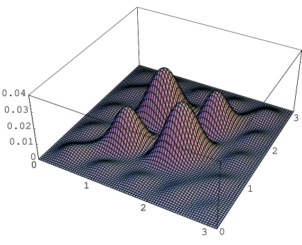
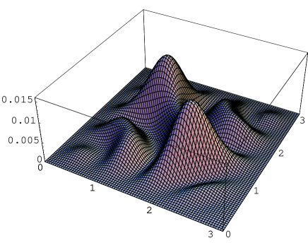
Figure 1: Probability distribution $p(\theta_{1},\theta_{2},\varphi=\pi/2)$ and $p(\theta_{1},\theta_{2},\varphi=\pi/21)$ for $j_{1}=j_{2}=j_{3}=2$.

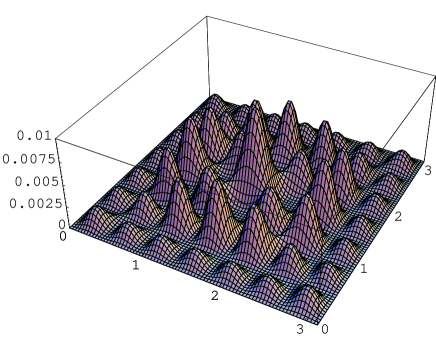
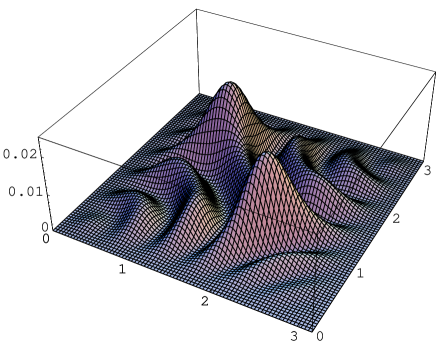
Figure 2: Probability distribution $p(\theta_{1},\theta_{2},\varphi=\pi/2)$ and $p(\theta_{1},\theta_{2},\varphi=\pi/21)$ for $j_{1}=j_{2}=j_{3}=3$.

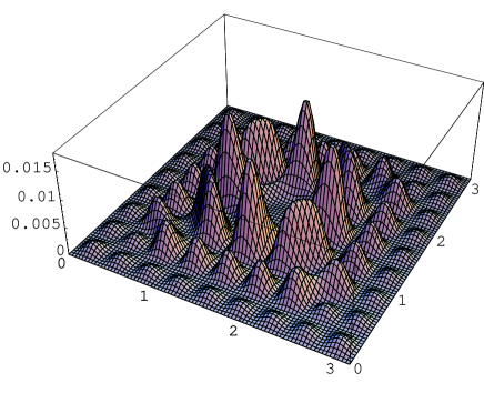
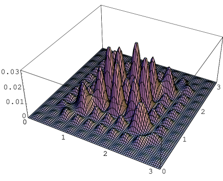
Figure 3: Probability distribution $p(\theta_{1},\theta_{2},\varphi=\pi/2)$ for $j_{1}=j_{2}=j_{3}=4$ and $j_{1}=j_{2}=j_{3}=6$.

In general, more complicated spin networks will have more complex probability graphs. A generic feature though is that the flat connection $\forall e\in\Gamma,\,g_{e}={\mathbbm{1}}$ will have a vanishing probability (density). Nevertheless, when the spins $j_{e}$ grows to $\infty$, it is likely that we obtain maxima arbitrarily close to the flat configuration (like in the case of a single Wilson loop).

Let us emphasize that these are only “kinematical” probabilities, based on the kinematical scalar product. “Physical” probabilities would be based on the physical scalar product taken into account the projection onto the kernel of the Hamiltonian constraint. The kinematical probabilities describe the unconstrained 3d space geometry, whereas the physical probabilities should implement the canonical constraints imposed by general relativity on the 3d geometry and should reflect the dynamical transition amplitudes induced by the Hamiltonian constraint.

In the present work, we aim to understand the geometry and structure of the quantum 3d geometry states, or spin networks, at the kinematical level. Indeed, before implementing the Hamiltonian constraints or the Einstein equations at the classical level, we first have to grasp the notion of metric. Here, we would like to understand the notion of quantum metric, before studying the solutions to the quantum constraint which should implement quantum gravity.

III Surface States and Area Renormalisation

Let us consider a surface ${\cal S}$ in the 3d space $\Sigma$ and a spin network state $|\Gamma,\vec{\jmath},{\vec{{\cal I}}}\rangle$ based on the graph $\Gamma$ considered as embedded in $\Sigma$. The surface intersects the graph at a certain number of points ${\cal S}\cap\Gamma=\{P_{1},..,P_{n}\}$ belonging to the graph edges $P_{i}\in e_{i}$. We then cut the surface ${\cal S}$ in elementary patches ${\cal S}_{i}$ intersecting $\Gamma$ at the points $P_{i}$: ${\cal S}=\coprod_{i}{\cal S}_{i}$ with ${\cal S}_{i}\cap\Gamma=P_{i}$. The area (operator) of ${\cal S}$ is defined as the sum of the areas (operators) of the elementary patches:

$$\widehat{{\cal A}}_{\cal S}\,|\Gamma,\vec{\jmath},{\vec{{\cal I}}}\rangle\,\equiv\,l_{P}^{2}\sum_{i}S(j_{e_{i}})\,|\Gamma,\vec{\jmath},{\vec{{\cal I}}}\rangle.$$ (13)

This simple definition of the area operator of a surface ${\cal S}$ in LQG raises two natural issues, due to the background independence of the theory. The first question is the definition of the surface itself in the diffeomorphism-invariant framework of LQG. Indeed, forgetting about the embedding of ${\cal S}$ and $\Gamma$ in the space manifold $\Sigma$, the surface ${\cal S}$ is defined on the spin network state $|\Gamma,\vec{\jmath},{\vec{{\cal I}}}\rangle$ only through its intersections $P_{i}$ with the graph $\Gamma$. Starting with a quantum geometry defined solely from the state $|\Gamma,\vec{\jmath},{\vec{{\cal I}}}\rangle$, independently from any metric or embedding or reference to $\Sigma$, one can define a (quantum) surface as a set of edges $e_{1},..,e_{n}$ of the graph $\Gamma$: the surface is then definedas the union of elementary patches ${\cal S}_{i}$ transversal to each edge $e_{i}$. However, how can we know that these patches are close to each over and that they do form a smooth continuous surface? The second question is related and concerns the semi-classical limit of such a quantum surface. More precisely, we would like to know how the surface is folded, i.e how the elementary patches are organized with respect to each other. Since these elementary patches might be crumpled giving a fractal-like structure to the surface, we would like to be able to coarse-grain the surface, define its macroscopic structure and its macroscopic area.

Following the preliminary ideas in ourbh , we will propose a framework of area renormalisation to address these issues and we will define coarse-grain area operators to probe the quantum structure of a surface.

Let us fix a graph $\Gamma$ and an arbitrary quantum state defined as the cylindrical function $\psi_{\Gamma}(g_{e})$. Let us consider the quantum surface defined as the set of edges $\{e_{1},..,e_{n}\}$. The area operator $\widehat{{\cal A}}_{i}$ of the elementary surface ${\cal S}_{i}$ transversal to the edge $e_{i}$ is defined as the Casimir operator of the following $\mathrm{SU}(2)$ action on $\psi_{\Gamma}(g_{e})$:

$$(g_{e_{i}},g_{e\neq e_{i}})\,\underset{g\in\,\mathrm{SU}(2)}{\longrightarrow}\,(gg_{e_{i}},g_{e\neq e_{i}}).$$ (14)

In this simple case, it doesn’t matter whether we act by left or right multiplication. It is natural to generalize this area operator to collections of elementary surfaces. Indeed, let us group together the edges $e_{1}$ and $e_{2}$. We define the coarse-grained area operator $\widehat{{\cal A}}_{(12)}$ as the Casimir operator of the diagonal $\mathrm{SU}(2)$ action:

$$(g_{e_{1}},g_{e_{2}},g_{e\neq e_{1},e_{2}})\,\underset{g\in\,\mathrm{SU}(2)}{\longrightarrow}\,(gg_{e_{1}},gg_{e_{2}},g_{e}).$$ (15)

This is easily generalized to any collection of edges. For example, the complete coarse-grained area operator $\widehat{{\cal A}}_{1..n}$ of the surface ${\cal S}$ is defined as the Casimir operator of the diagonal $\mathrm{SU}(2)$ action:

$$(g_{e_{1}},g_{e_{2}},..,g_{e_{n}},g_{e\neq e_{1},..,e_{n}})\,\underset{g\in\,\mathrm{SU}(2)}{\longrightarrow}\,(gg_{e_{1}},gg_{e_{2}},..,gg_{e_{n}},g_{e}).$$ (16)

It is now necessary to distinguish the left and right multiplication. We actually define $2^{n}$ different operators. Not only we can define the two operators, $\widehat{{\cal A}}_{(12)}^{(L)}$ and $\widehat{{\cal A}}_{(12)}^{(R)}$, corresponding to the actions $(g_{1},g_{2})\rightarrow(gg_{1},gg_{2})$ and $(g_{1},g_{2})\rightarrow(g_{1}g,g_{2}g)$, but we must also consider the two other actions $(g_{1},g_{2})\rightarrow(gg_{1},g_{2}g^{-1})$ and $(g_{1},g_{2})\rightarrow(g_{1}g^{-1},gg_{2})$.

The key point is that $\widehat{{\cal A}}_{(12)}\,\psi_{\Gamma}\neq\left(\widehat{{\cal A}_{1}}+\widehat{{\cal A}_{2}}\right)\,\psi_{\Gamma}$ and this results in a non-trivial flow of the area of a surface under coarse-graining. Let us consider the simple example of a spin network state with the edges $e_{1,2}$ labelled with the representations $j_{1}=1000$ and $j_{2}=1007$. The microscopic area of the surface ${\cal S}\equiv\{e_{1},e_{2}\}$ is ${\cal A}_{\rm micro}=S(1000)+S(1007)$ in Planck unit. Now assuming that these two edges meet at a 3-valent vertex as in fig. 4 and that the third edge is labelled with the representation $j=12$, then the macroscopic (coarse-grained) area of the same surface ${\cal S}$ will be ${\cal A}_{\rm macro}=S(12)$ which is substantially different.

\psfrag{j}{$j=12$}\psfrag{j1}{$j_{1}=1000$}\psfrag{j2}{$j_{2}=1007$}\psfrag{S}{${\cal S}$}\includegraphics[width=142.26378pt]{1000to12.eps}

Figure 4: Considering a surface ${\cal S}=\{e_{1},e_{2}\}$ made of two spin network edges labelled by spins $j_{1}=1000$ and $j_{2}=1007$, the microscopic area is $S(1000)+S(1007)$ while the coarse-grained area $S(12)$ is much smaller and takes into account the nearby intertwiner describing the coupling between the two representations $j_{1}$ and $j_{2}$.

We propose to use the coarse-graining flow, or renormalisation flow, of the surface area to probe the structure of the surface. A possible coarse-graining of the surface ${\cal S}=\{e_{1},..,e_{n}\}$ is summarized by a tree $T$ which describes how we group the edges together: each level of the tree defines a partition of $\{e_{1},..,e_{n}\}$ which is coarser than the previous level, from the initial point with individual edges to the final point when all the edges are grouped together. The coarse-grained area (operator) of the surface ${\cal S}$ at each level depends on the partition and is defined as the sum of the area operators of each collection of edges of the given partition. Then each tree $T$ describes a possible coarse-graining of the surface ${\cal S}$ from the microscopic realm to the macroscopic level. Given a state of geometry $\psi_{\Gamma}$, we can analyze the renormalisation flow of the expectation value of the area for each coarse-graining tree $T$.

For some trees the flow may be smooth, meaning that transitions from a level to a neighboring lead to small changes in area in Planck units, while it might be jumpy for the other trees. We expect that if there does not exist any tree with smooth flow, then the set of chosen edges can not describe a true surface in the macroscopic limit and that these edges are likely to be far from each other in the geometry defined by the state $\psi_{\Gamma}$. On the other hand, a tree with a smooth flow should give us the right way to put the elementary surfaces together grouping them by closest neighbors. Moreover, we expect that such a (smooth) area flow tells us more about the properties of the surface such as its curvature. For example, a (nearly) flat surface should have a almost trivial constant area flow.

This proposes an explicit relationship between the geometry of a spin network state and its renormalisation properties. This will be investigated in more details through specific examples in future work elisa . A similar analysis of the volume renormalisation flow should carry even more information about the geometry of the quantum state $\psi_{\Gamma}$.

This is to be compared with theories on the lattice. Renormalisation à la Wilson is defined through coarse-graining the lattice and deriving the flow of the Hamiltonian and of the various observables under that coarse-graining operation. Usually, the lattice is embedded in flat space and the coarse-graining defined through the resulting notion of nearest neighbor. In our quantum gravity context, spin networks can be thought as a lattice. However, there are provided without any embedding into a space manifold. Our proposal is to consider all the possible renormalisation flow of geometrical observables (such as the area) and to reconstruct a “correct” embedding by identifying the “good” renormalisation flow(s). The whole issue is then to define what we mean by “good”. The simplest criteria is the smoothness of the flow. However, this should be studied in more details.

In the case of a (pure) spin network state $\psi_{\Gamma}=\,|\Gamma,\vec{\jmath},{\vec{{\cal I}}}\rangle$, we can give a simple expression of the expectation value of a coarse-grained area operator. Let us consider the collection of edges $\{e_{1},..,e_{n}\}$ and the Casimir operator of the diagonal $\mathrm{SU}(2)$ action $(g_{e_{1}},g_{e_{2}},..,g_{e_{n}})\rightarrow(gg_{e_{1}},gg_{e_{2}},..,gg_{e_{n}})$ where we act at the source vertex of all edges. Considering the action where $g$ sometimes acts at the target vertex would not change much to the following.

Using the kinematical scalar product on the spin networks defined by the integration with the Haar measure, we show that the area expectation value is given by:

$$\langle\widehat{{\cal A}}_{(e_{1},..,e_{n})}\rangle_{\psi}\,=\,\frac{{\rm tr}\,\,\vec{J}^{2}\,\rho}{{\rm tr}\,\rho},$$ (17)

where $\rho$ is a density matrix describing the state of the surface $e_{1},..,e_{n}$ in the Hilbert space $\otimes_{i}V^{j_{e_{i}}}$. $\rho$ is defined in terms of the intertwiners ${\cal I}_{v}$ of the spin network at the vertices where we act with $g$, i.e $v=s(e_{1}),..,s(e_{n})$:

$$\rho_{a_{1}..a_{n}b_{1}..b_{n}}\,\equiv\,\prod_{i}{\rm tr}\,\left[\overline{{\cal I}_{v=s(e_{i})}}{}^{a_{i}}\,{\cal I}_{v=s(e_{i})}{}^{b_{i}}\right],$$ (18)

where $a_{i},b_{i}$ label a basis of the representation space $V^{j_{e_{i}}}$. The trace is over the representation space associated to the edges $e$ not belonging to the surface $\{e_{1},..,e_{n}\}$. An example is given in fig. 5. $\rho$ is hermitian and generically represents a mixed state.

\psfrag{1}{$e_{1}$}\psfrag{2}{$e_{2}$}\psfrag{3}{$e_{3}$}\psfrag{S}{${\cal S}$}\psfrag{A}{$A$}\psfrag{B}{$B$}\includegraphics[width=142.26378pt]{3edgesurf.eps}

Figure 5: Considering a surface ${\cal S}=\{e_{1},e_{2},e_{3}\}$ made of three spin network edges labelled by representations $j_{1,2,3}$, the surface state relevant for the (coarse-grained) area expectation values is the mixed state on the Hilbert space $V^{j_{1}}\otimes V^{j_{2}}\otimes V^{j_{3}}$ defined by the density matrix $\rho_{a_{i}b_{i}}=\overline{{\cal I}_{A}}^{a_{1}a_{2}\alpha}{\cal I}_{A}^{b_{1}b_{2}\alpha}\overline{{\cal I}_{B}}^{a_{3}\beta\gamma}{\cal I}_{B}^{b_{3}\beta\gamma}$. It depends on the intertwiners living at the vertices $A$ and $B$ at the source of the edges $e_{1,2,3}$.

From the above expression for the surface state, it is clear that the coarse-graining procedure probes the structure of the spin network around the considered surface, for instance the intertwiners attached to the vertex adjacent to the surface. These intertwiners describe how the surface is folded, i.e the ”position” of the elementary patches with respect to each other. If we were to use a more complicated scalar product between spin network states, taking into account some dynamical effect and propagation of the geometry degrees of freedom, it is likely that the coarse-grained area expectation value would involve intertwiners attached to further vertices and would depend in a more complex way on the spin network geometry.

We conclude this section with a simple example of area renormalisation. We consider three edges $e_{1,2,3}$ all labelled by the fundamental representation $j=\frac{1}{2}$. The representation space $V^{1/2}$ is two-dimensional and we write the two basis vector of maximal and minimal weights as $|\uparrow\rangle,|\downarrow\rangle$. Let us consider the surface state defined as the pure state $\rho=|\uparrow\uparrow\downarrow\rangle\langle\uparrow\uparrow\downarrow|$. Then the microscopic area in Planck unit is obviously:

$$\langle\widehat{{\cal A}}_{123}\rangle=3\,S\left(\frac{1}{2}\right)\sim 2.598,$$

where the numerical value is computed using the spectrum $S(j)=\sqrt{j(j+1)}$. The coarse-grained areas, the one grouping the edges 1,2 together and the other grouping the edges 2,3 together are easily computed:

$$\langle\widehat{{\cal A}}_{(12)3}\rangle=S(1)+S\left(\frac{1}{2}\right)\sim 2.280,$$

$$\langle\widehat{{\cal A}}_{1(23)}\rangle=S\left(\frac{1}{2}\right)+\frac{1}{2}\left(S(1)+S\left(\frac{1}{2}\right)\right)\sim 2.006.$$

Finally the totally coarse-grained area grouping all three edges 1,2,3 together is given by:

$$\langle\widehat{{\cal A}}_{(123)}\rangle=\frac{1}{3}S\left(\frac{1}{2}\right)+\frac{2}{3}S\left(\frac{1}{2}\right)\sim 1.223.$$

We can not really introduce a notion of smooth flow for such a small surface with so few edges. We would need a much larger surface, for which the state $\rho$ would inevitably be much more complicated and analytical computations more involved elisa . Nevertheless, there is one state which can easily studied. It is the pure state for $n$ edges, $\rho=|\uparrow..\uparrow\rangle\langle\uparrow..\uparrow|$. Its renormalisation flow is practically constant. If we partition/group the set of $n$ edges into packets of size $\alpha_{i}$, $\sum_{i}\alpha_{i}=n$, then the corresponding coarse-grained area is:

$$\langle\widehat{{\cal A}}_{\{\alpha_{i}\}}\rangle=\sum_{i}S\left(\frac{\alpha_{i}}{2}\right).$$

The microscopic area is $\langle\widehat{{\cal A}}_{\rm micro}\rangle=nS(\frac{1}{2})$ while the macroscopic area is $\langle\widehat{{\cal A}}_{\rm micro}\rangle=S(\frac{n}{2})$. If we use the simpler spectrum $\widetilde{S}(j)=j$, the renormalisation is actually exactly constant.

IV Coarse-Graining: from Bulk to Boundary

Considering a bounded region $A$ of a spin network state, we are interested by the boundary state(s) on $\partial A$ induced by the quantum state of geometry of the bulk of $A$ (or by the region outside the region $A$). We will see the boundary state can be considered as a coarse-graining of the geometry state of $A$ and be constructed from partial tracing of the bulk degrees of freedom.

IV.1 Coarse-graining: definition

Let us consider quantum states based on a fixed given graph $\Gamma$, which we assume closed and connected, and a bounded connected region $A$ of this spin network which we define as a set of vertices in $\Gamma$.

An edge $e$ is considered in $A$ if both its source and target vertices are in $A$, $s(e),t(e)\in A$. We define the boundary $\partial A$ of the region $A$ as the set of edges with one vertex in $A$ and one vertex outside $A$. For every couple of vertices $v_{1},v_{2}$ in $A$ there exists a path of edges in $A$ linking them. Moreover, if one cuts in two all the edges in the boundary $\partial A$, then one cuts the graph $\Gamma$ in two connected open graphs. We will call $\Gamma_{A}$ the connected open graph with all the vertices in $A$ and ending at the boundary $\partial A$. Finally, we call $\breve{A}$ the exterior of $A$ i.e the set of vertices and edges who do not belong to $A$ and its boundary $\partial A$.

For the sake of the simplicity of the notations, we assume in the following that all the edges $e\in\partial A$ on the boundary are identically oriented outward, with $s(e)\in A$ and $t(e)\notin A$.

The boundary state of $A$ is the state of the edges $e\in\partial A$ irrespectively of the details of the structure of the graph $\Gamma_{A}$ inside the region $A$. We can therefore think about it as the coarse-grained state of $A$ once we coarse-grain the whole interior graph of $A$ to a single vertex. Let us thus define the graph $\Gamma[A]$ where we have removes the whole graph $\Gamma_{A}$ from $\Gamma$ and replaced it by a single vertex, as in Fig.6.

Figure 6: Coarse-graining the region $A$ to a single vertex: from the graph $\Gamma$ to the reduced graph $\Gamma[A]$.

We then define the following coarse-graining map.

Definition 1.

We define a coarse-graining map $\Theta:H_{\Gamma}\rightarrow H_{\Gamma[A]}$ taking cylindrical functions defined on the full graph $\Gamma$ to cylindrical functions defined on the reduced graph $\Gamma[A]$:

$$(\Theta\,\psi)(\{g_{e},e\in\Gamma[A]\})\,\equiv\,\int_{\mathrm{SU}(2)}dg\,\psi(\{g_{e\in\breve{A}},gg_{e\in\partial A},g^{(0)}_{e\in A}\}).$$ (19)

The integration over $g$ is to ensure the proper gauge invariance of the resulting functional. The map $\Theta$ actually depends on the group elements $g^{(0)}_{e\in A}\in\mathrm{SU}(2)$, which need to be fixed. We call them the coarse-graining data. We call the trivial or canonical coarse-graining map the one defined by $g^{(0)}_{e\in A}={\mathbbm{1}}$. For this canonical choice, the integration over $\mathrm{SU}(2)$ is irrelevant and we can drop it.

Due to the gauge invariance of the initial functional $\psi$, the coarse-graining data $g^{(0)}_{e\in A}$ is actually defined up to $\mathrm{SU}(2)$ actions at each vertex of $A$. As a result, the coarse-graining data lives in the quotient space $X_{A}\,\equiv\,\mathrm{SU}(2)^{E_{A}}/\mathrm{SU}(2)^{W_{A}+1}$, where $W_{A}$ is the number of vertices in $A$ who do not have any edge on the boundary.

It is useful to look at this coarse-graining procedure in the case of a (pure) spin network state. The spin network state labels each edge $e$ of the graph with a (irreducible) representation $j_{e}$. The state of the bulk of the region $A$ is given by the intertwiners attached to the vertices of $A$, and lives in the Hilbert space ${\cal H}_{A}\,\equiv\,\otimes_{v\in A}{\rm Int}_{v}$. The state of the boundary $\partial A$ lives in the tensor product $\otimes_{e\in\partial A}V^{j_{e}}$. We require it to be $\mathrm{SU}(2)$ invariant so that the boundary Hilbert space is ${\cal H}_{\partial A}\,\equiv\,{\rm Int}(\otimes_{e\in\partial A}j_{e})$. The coarse-graining is a map from ${\cal H}_{A}$ to ${\cal H}_{\partial A}$: we glue the intertwiners inside $A$ together in order to obtain an intertwiner solely between the edges on the boundary of $A$. This procedure is equivalent to the construction described above and effectively reduces the whole interior graph of $A$ to a single vertex.

More precisely, given some fixed holonomies along the edges of $A$, we can define the coarse-grained intertwiner as follow.

Definition 2.

Given the coarse-graining data $\{g^{(0)}_{e\in A}\}$, and intertwiners ${\cal I}_{v\in A}\in{\cal H}_{A}$, we define the following coarse-grained intertwiner in ${\cal H}_{\partial A}$:

$${\cal I}_{A}[g^{(0)}_{e\in A}]\,\equiv\,\int_{\mathrm{SU}(2)}dg\,{\rm tr}\,_{e\in A}\,\left[\bigotimes_{e\in\partial A}D^{j_{e}}(g)\bigotimes_{e\in A}D^{j_{e}}(g^{(0)}_{e})\bigotimes_{v\in A}{\cal I}_{v}.\right]$$ (20)

The integration over $\mathrm{SU}(2)$ is to impose $\mathrm{SU}(2)$ invariance and obtain an intertwiner at the end of the day. The canonical choice $\{g^{(0)}_{e\in A}={\mathbbm{1}}\}$ amounts to straightforwardly gluing the intertwiners. In that case, we automatically respect gauge invariance and we obtain an intertwiner without having to integrate over $\mathrm{SU}(2)$.

More details on the motivation for this definition of coarse-graining from the point of view of partial tracing and the uniqueness of the procedure are given in appendix.

Due to the gauge invariance, the coarse-grained intertwiner actually depends only on the orbit of $\{g^{(0)}_{e\in A}\}$ under $\mathrm{SU}(2)$ transformations: it is defined in terms of $x\in X_{A}=\mathrm{SU}(2)^{E_{A}}/\mathrm{SU}(2)^{W_{A}+1}$.

Example 3.

Let us explain the simple example of a 4-punctured boundary $V_{j_{1}}\otimes V_{j_{2}}\rightarrow V_{j_{3}}\otimes V_{j_{4}}$ with the internal graph being made of two 3-valent vertices and a single internal edge labelled with a fixed spin $j$. The two intertwiners attached to the two 3-valent vertices are unique and given by the usual Clebsh-Gordan coefficients. Coarse-graining means assigning a group element to the internal edge and integrating over an orbit under the adjoint action $Ad(\mathrm{SU}(2))$. An orbit in $\mathrm{SU}(2)/Ad(\mathrm{SU}(2))$ is defined by an angle $\theta\in]-\pi,\pi]$ and is the equivalence class of the group element $h_{\theta}\equiv\exp(i\theta J_{z})$. The corresponding coarse-grained intertwiner ${\cal I}^{\theta}:V_{j_{1}}\otimes V_{j_{2}}\rightarrow V_{j_{3}}\otimes V_{j_{4}}$ becomes

$${\cal I}^{\theta}_{m_{1}m_{2}m_{3}m_{4}}=\int_{\mathrm{SU}(2)}dg\,C^{j_{3}j_{4}j}_{m_{3}m_{4}n}D^{j}_{mn}(gh_{\theta}g^{-1})C^{j_{1}j_{2}j}_{m_{1}m_{2}m}.$$ (21)

We can evaluate exactly the integral over $g$:

$$\int_{\mathrm{SU}(2)}dg\,D^{j}_{mn}(gh_{\theta}g^{-1})=\delta_{mn}\frac{\chi^{j}(\theta)}{2j+1}.$$ (22)

We obtain that ${\cal I}^{\theta}={\cal I}^{0}\,\chi^{j}(\theta)/(2j+1)$ always leads to the same intertwiner defined at $\theta=0$ up to a normalization factor: the coarse-graining procedure is trivial in this simple setting. If the Clebsh-Gordan coefficients are normalized, then the norm of ${\cal I}^{\theta=0}$ is 1. As we will see later, the reason why the coarse-graining procedure is trivial is that the topology of the interior graph (here a single edge) is trivial. Coarse-graining will give a non-trivial result only when the interior graph has a non-trivial topology and contains at least one loop.

We now would like to extend these intertwiner definitions from a (pure) spin network state to an arbitrary cylindrical function. We need to decompose the cylindrical function onto the spin network basis, coarse-grain each spin network component separately, and then sum the coarse-grained components back to obtain the coarse-grained cylindrical function. This is equivalent to the definition def.1 of coarse-graining, since the procedure is a linear functional only involving integrating over part of the degrees of freedom of the wave-function (the holonomies on the edges of $A$). Nevertheless, we ought to consider the same coarse-graining data for all the spin network components of the initial functional. However, it might happen that it seems more suited to consider different data for each component, depending on the structure of each spin network state.

IV.2 The most probable coarse-graining?

The natural issue following the previous definition is how to choose the coarse-graining data. Indeed a priori, the coarse-grained state is a mixed state reflecting all the possible coarse-grainings given by the density matrix:

$$\rho_{A}\equiv\int_{X_{A}}d\mu(x)\,|{\cal I}_{A}[x]\rangle\langle{\cal I}_{A}[x]|.$$ (23)

A priori the measure $\mu(x)$ is simply the Haar measure on $X_{A}=\mathrm{SU}(2)^{E_{A}}/\mathrm{SU}(2)^{W_{A}+1}$. This density matrix comes explicitly from tracing out the holonomies along the edges within the region $A$.

A first remark is that this density matrix is in general not the totally mixed state ${\mathbbm{1}}_{\partial A}/{\rm dim}{\cal H}_{\partial_{A}}$. Therefore, our coarse-graining procedure does not erase all the information about the internal state of the region $A$. Obtaining the totally mixed state by averaging over all possible ways of coarse-graining would thus require a special quantum state. We expect this to be related to quantum black holes ourbh .

The second remark is that the coarse-grained procedure does not provide us with normalized intertwiners $||{\cal I}_{A}[x]||\neq 1$. Following the interpretation of the spin network functional as a wave function defining a probability amplitude on the holonomies, this norm $||{\cal I}_{A}[x]||^{2}$ actually provides us with a measure of the probability on the space of possible coarse-grainings $X_{A}$. Indeed, the coarse grained intertwiner ${\cal I}_{A}[x]$, or equivalently the coarse grained state defined in def.1, are defined simply by evaluating the initial spin network on the holonomies $x=\{g^{(0)}_{e\in A}\}$. This means that, although it seems more natural to coarse-grain using the canonical choice $x={\mathbbm{1}}$, that might not be the most probable holonomies inside the region $A$.

To summarize the situation, let us assume that we work with normalized spin network functionals i.e that all the intertwiners ${\cal I}_{v}$ are normalized, $||{\cal I}_{v}||=1$. Now the density matrix describing the coarse-grained geometry of the region $A$ is:

$$\rho_{A}=\int_{X_{A}}d\mu(x)\,|{\cal I}_{A}[x]\rangle\langle{\cal I}_{A}[x]|=\int_{X_{A}}||{\cal I}_{A}[x]||^{2}\,d\mu(x)\,|\widetilde{{\cal I}}_{A}[x]\rangle\langle\widetilde{{\cal I}}_{A}[x]|,$$

where $\widetilde{{\cal I}}_{A}[x]$ is now the normalized intertwiner describing the geometry of the region $A$ reduced to a single vertex. Clearly the probability distribution on this intertwiner is given by the measure $||{\cal I}_{A}[x]||^{2}\,d\mu(x)$.

We can finally generalize these considerations to an arbitrary cylindrical function. The coarse-grained state will similarly be described by the density matrix,

$$\rho_{A}(\psi)\,\equiv\,\int dx|\Theta_{x}\psi\rangle\langle\Theta_{x}\psi|,$$

and the most probable coarse-grainings will be defined as the maxima of the norm of the coarse-grained functional $||\Theta_{x}\psi||^{2}$.

IV.3 Coarse-graining data, gauge fixing and non-trivial topology

To understand the structure and relevance (or irrelevance) of the coarse-graining data, it is useful to explicitly gauge-fix the initial functional $\varphi$. This is he simplest way to see how the whole graph inside $A$ gets reduced to a single vertex.

Indeed, following noncompact , we choose a (reference) vertex $v_{0}$ in $A$ and a maximal tree $T$. $T$ is a set of edges in $A$ going through all vertices of $A$ without ever making any loop. It has $|T|=V_{A}-1$ elements. If $|T|=E_{A}$, this means that the interior graph $\Gamma_{A}$ has no loop and has a trivial topology. $E_{A}-|T|$ counts the number of non-trivial loops of $\Gamma_{A}$. We know that we can use the gauge invariance to fix to the identity the group elements on the edges belonging to the tree, $g_{e\in T}={\mathbbm{1}}$,

$$\psi(\{g_{e\in\breve{A}},g_{e\in\partial A},g_{e\in A}\})\,=\,\psi(\{g_{e\in\breve{A}},H_{e}g_{e\in\partial A},{\mathbbm{1}}_{e\in T},G_{e\in A\setminus T}\}).$$

To define $G$ and $H$, we define for every vertex $v\in A$ the unique path ${\cal L}_{v}$ along $T$ from $v_{0}$ to $v$. Then we define the group element:

$$H_{v}\,\equiv\,\overrightarrow{\prod_{e\in{\cal L}_{v}}}g_{e}.$$

Finally, $H_{e\in\partial A}\,\equiv\,H_{s(e)}$ and $G_{e\in A\setminus T}\,\equiv\,H_{s(e)}g_{e}H_{t(e)}^{-1}$.

The $H_{e\in\partial A}$ can be considered as irrelevant for the coarse-graining since that they can be re-absorbed in the redefinition of the holonomies $g_{e\in\partial A}$ on the boundary of $A$. On the other hand, the group elements $G_{e\in A\setminus T}$ can not be forgotten and actually represent the holonomies around each (non-contractible) loop of the interior graph $\Gamma_{A}$. They therefore reflect the non-trivial topologyof the quantum state of geometry of $A$.

Having set the maximal number of holonomies to the identity inside $A$, we have effectively reduced the whole graph $\Gamma_{A}$ to a single vertex (the vertex $v_{0}$) with $n$ open edges (with $n=|\partial A|$ is the number of edges in the boundary) and $L_{A}$ loops. The number of loops is simply $L_{A}=E_{A}-V_{A}+1$. See fig.7 for an example with two loops.

\psfrag{j1}{$j_{1}$}\psfrag{j2}{$j_{2}$}\psfrag{ja}{$j_{a}$}\psfrag{jb}{$j_{b}$}\includegraphics[width=170.71652pt]{LoopToPetal.eps}

Figure 7: Gauge-Fixing of a region with two loops: the graph has $|\partial A|=4$ external edges, $E_{A}=7$ internal edges, $V_{A}=6$ vertices, $L_{A}=E_{A}-V_{A}+1=2$ loops. We gauge fix along the tree $T$ in bold and contract the whole internal graph to a single vertex. That vertex defines an intertwiner $V^{j_{1}}\otimes\cdots\otimes V^{j_{4}}\otimes(V^{j_{a}})^{\otimes 2}\otimes(V^{j_{b}})^{\otimes 2}\rightarrow\mathbb{C}$. The coarse-graining data is then the holonomies around the two loops ${\cal L}_{a},{\cal L}_{b}$.

Contracting all the vertices of $A$ to a single one, and gluing all the corresponding intertwiners together putting the identity on the edges of the tree $T$, lead a single intertwiner ${\cal I}:V^{\otimes n}\otimes V^{\otimes 2L_{A}}\rightarrow\mathbb{C}$. Here we write $V$ to refer to which ever representation $V^{j}$ lives on the considered edge (or loop). The region $A$ is then described by the contraction of this single intertwiner with the holonomies $G_{e\in A\setminus T}$ along the loops. Labelling the loops by $i=1..L_{A}$ and noting the corresponding holonomies $G_{i}$, the functional reads:

$${\cal I}_{\alpha_{1}..\alpha_{n}\,a_{1}b_{1}..a_{L_{A}}b_{L_{A}}}\,\prod_{i}^{L_{A}}D_{a_{i}b_{i}}(G_{i}).$$ (24)

Coarse-graining this structure amounts to reduce the whole graph to a single vertex without any loop. From this point of view, it is clear that a non-trivial coarse-graining of the region $A$ corresponds to a non-trivial topology of the graph $\Gamma_{A}$ inside the region $A$. The relevant coarse-graining data is an element of the group $\mathrm{SU}(2)^{L_{A}}=\mathrm{SU}(2)^{E_{A}-V_{A}+1}$ i.e one holonomy for each loopin $A$. When $E_{A}=V_{A}-1$, there is no loop in $A$ and we are left with the trivial coarse-graining setting all holonomies on the edges in $A$ to the identity. Coarse-graining thus amounts to erase any non-trivial topology of the graph of the geometry state of $A$.

We coarse-grain by averaging over the loop holonomies with an arbitrary function $\Phi(G_{1},..,G_{L_{A}})\in L_{2}(\mathrm{SU}(2)^{L_{A}})$:

$$\int\prod_{i}dG_{i}\,\Phi(G_{1},..,G_{L_{A}}){\cal I}_{\alpha_{1}..\alpha_{n}\,a_{1}b_{1}..a_{L_{A}}b_{L_{A}}}\,\prod_{i}^{L_{A}}D_{a_{i}b_{i}}(G_{i}).$$ (25)

We require that the result after integration is still an intertwiner $V^{\otimes n}\rightarrow\mathbb{C}$, i.e invariant under (the diagonal action of) $\mathrm{SU}(2)$ (on $\alpha_{1}..\alpha_{n}$). This imposes that $\Phi(G_{1},..,G_{L_{A}})$ be invariant under the adjoint action of $\mathrm{SU}(2)$,

$$\Phi(G_{1},..,G_{L_{A}})=\Phi(gG_{1}g^{-1},..,gG_{L_{A}}g^{-1}).$$

This means that $\Phi$ is a spin network functional on the flower graph with $L_{A}$ petals -see fig.7 for an example with a two-petal flower.

Now, one could look for coarse-graining data which maximizes the (norm of the) coarse-grained intertwiner, either directly as (an orbit) $Ad(\mathrm{SU}(2)).(G_{1}^{(0)},..,G_{L_{A}}^{(0)})$, or equivalently as a $Ad(\mathrm{SU}(2))$-invariant functional $\Phi$. If we do not consider $Ad(\mathrm{SU}(2))$-invariant coarse-graining data, we will not obtain an intertwiner as result of the coarse-graining, but more generally a vector in the tensor product $V^{\otimes n}$.

An alternative to imposing by hand to obtain an intertwiner after coarse-graining would to look for maxima among all coarse-graining data $(G_{1}^{(0)},..,G_{L_{A}}^{(0)})$, possibly non-invariant. If the most probable holonomies along the loops are actually the identity (or at least very close to it), then we get simply set them to ${\mathbbm{1}}$ in the coarse-graining procedure and erase the non-trivial topology of the graph. If the probability is actually peaked around non-trivial values of the holonomies, this could mean that the non-trivial topology of the graph truly reflect a non-trivial topology of the region $A$ and that we should not neglect the contribution/couplings of the loops to the intertwiner. In that case, our coarse-graining procedure, which erases the non-trivial topology, might not reflect the true geometry of the region $A$.

At the end of the day, we have seen how the coarse-graining procedure can be understood as “erasing” the non-trivial topology of the region $A$ (more precisely, the topology of the graph underlying the quantum state of geometry of the region $A$) through integrating over the degrees of freedom attached to the internal edges of the region $A$.

IV.4 Inside state vs. outside state

Considering a pure spin network state $|\Gamma,\vec{\jmath},{\vec{{\cal I}}}\rangle$ and given a region $A$ of that spin network and an assignment $x\in X_{A}$ of groups elements to each internal edge, we have seen to define a boundary state ${\cal I}_{A}(x)\in{\cal H}_{\partial A}$. Since we are studying a spin network state based on a closed graph, the exterior of $A$ defines a (complementary) region of the spin network with the same boundary. Defining the quotient space $Y_{A}\equiv X_{\breve{A}}$ of all possible coarse-grainings of the exterior of $A$, each element $y\in Y_{A}$ induces a boundary state ${\cal I}_{A}^{{\rm ext}}(y)\in{\cal H}_{\partial A}$, which is a priori arbitrarily different from the states ${\cal I}_{A}^{{\rm int}}(x)$ obtained by coarse-graining the interior of $A$. Let us point out that ${\cal I}_{A}^{{\rm ext}}(y)$ is actually in $\overline{{\cal H}_{\partial A}}$ (because of the reverse orientation of the edges), which is nevertheless isomorphic to ${\cal H}_{\partial A}$ since we work with $\mathrm{SU}(2)$.

At the intuitive level, one can see the boundary state ${\cal I}_{A}^{{\rm int}}(x)$ as the state of $\partial A$ induced by the (quantum) metric inside $A$ while ${\cal I}_{A}^{{\rm ext}}(y)$ is the boundary state induced by the outside (quantum) metric. Then we can look for transition functions (or transition amplitudes) allowing to go from ${\cal I}_{A}^{{\rm int}}(x)$ to ${\cal I}_{A}^{{\rm ext}}(y)$. More precisely, we would like to identify a function $\varphi_{x,y}(\{g_{e},e\in\partial A\})$ such that:

$${\cal I}_{A}^{{\rm ext}}(y)=\int_{\mathrm{SU}(2)^{|\partial A|}}\prod_{e\in\partial A}dg_{e}\,\varphi_{x,y}(\{g_{e},e\in\partial A\})\bigotimes_{e\in\partial A}D^{j_{e}}(g_{e}){\mathbf{.}}\,{\cal I}_{A}^{{\rm int}}(x).$$ (26)

This makes sense since ${\cal I}_{A}^{{\rm int}}(x)\in{\cal H}_{\partial A}={\cal H}^{0}(\bigotimes_{e\in\partial A}V_{j_{e}})$ lives in the tensor product $\bigotimes_{e\in\partial A}V_{j_{e}}$. Actually to be rigorous, we should write $\overline{{\cal I}_{A}^{{\rm ext}}}(y)$.

Such a transition amplitude $\varphi_{x,y}(\{g_{e},e\in\partial_{A}\})$ would reflect the curvature at the level of the surface $\partial A$, between the inside and the outside of $A$. Indeed it describes the parallel transport when crossing the surface $\partial A$.

A solution is actually given by the spin network functional itself $\phi_{(\Gamma,j_{e},{\cal I}_{v})}[g]$. Indeed a straightforward calculation gives that a suitable function for $x=\{G_{e},e\in A\}$ and $y=\{G_{e},e\in\breve{A}\}$ is defined as:

$$\varphi_{x,y}(\{g_{e},e\in\partial A\})\equiv\frac{1}{\|{\cal I}_{A}^{{\rm int}}(x)\|^{2}}\,\overline{\phi}\,(g_{e\in\partial A},G_{e\in A},G_{e\in\breve{A}}).$$ (27)

Since the spin network functional is actually the wave-function defining the probability amplitude for the connection and holonomies, this result fits with the intuition that the “transition function” $\varphi_{x,y}(\{g_{e},e\in\partial_{A}\})$ defines the probability amplitude for the curvature at the level of the surface $\partial A$.

IV.5 Coarse-graining of the Hilbert space: counting the degrees of freedom

We have seen previously that the coarse-graining of a region of a spin network is non-trivial only when the topology of the graph is non-trivial. We propose to look at this from the perspective of the dimension of the Hilbert space and see how the number of degrees of freedom get coarse-grained. More precisely, we investigate the dimensionality of the Hilbert space of bulk states once the structure of the boundary is fixed.

Considering the bounded region $A$ of the spin network, we look at the topology of the open graph $\Gamma_{A}$ inside $A$. If the graph $\Gamma_{A}$ is a single vertex, then the Hilbert space is simply the space of intertwiners between the representations $V^{j_{e}}$ attached to the edges on the boundary $e\in\partial A$:

$${\cal H}^{A}_{{\rm vertex}}\,=\,{\rm Int}(\bigotimes_{e\in\partial A}V^{j_{e}}).$$

If $\Gamma_{A}$ is more complicated and consists of many vertices and internal edges, a basis of the Hilbert space is given by a choice of representation labels for the internal edges $e\in A$ and of (orthogonal) intertwiner states for the internal vertices. This existence of intertwiners at the vertices imposes some restrictions on the possible representation labels (such as the triangular inequalities for trivalent vertices).

When $\Gamma_{A}$ has a trivial topology, i.e has no loops, then the Hilbert space is actually still isomorphic to the same intertwiner space:

$${\cal H}^{A}_{{\rm trivial}}\,=\,{\rm Int}(\bigotimes_{e\in\partial A}V^{j_{e}}).$$

Using a tree decomposition of a vertex is actually a standard way of constructing a basis of the intertwiner space.

As soon as $\Gamma_{A}$ has a non-trivial topology, i.e contains loops, the Hilbert space is a priori infinite-dimensional. Indeed, one can attach to each loop ${\cal L}$ with an un-constrained representation label $j_{\cal L}$. This is similar to the freedom of associating an arbitrary holonomy along each loop in the previous coarse-graining procedure. Since $j_{\cal L}$ is an arbitrary integer, the resulting Hilbert space has an infinite dimension. Thus one needs to gauge fix this freedom and fix the representation $j_{\cal L}$ -the flux around the loop- for each loop. Then the Hilbert space becomes finite-dimensional but still has a larger dimension than the intertwiner space.

Let us look at this in details in a simple example. We consider a region $A$ whose boundary comprises of $2n$ edges labelled with the fundamental representation $V^{1/2}$. It is rather straightforward to show that (see ourbh for example):

$$(V^{1/2})^{\otimes 2n}\,=\,\bigoplus_{k=0}^{n}\,(C^{n+k}_{2n}-C^{n+k+1}_{2n})\,V^{k},$$ (28)

where the $C$’s are the binomial coefficients. The dimension of the intertwiner space is the degeneracy of the spin-0 space:

$$\dim{\cal H}^{(2n)}_{{\rm trivial}}\,=\,C^{n}_{2n}-C^{n+1}_{2n}=\frac{1}{n+1}C^{n}_{2n}.$$ (29)

\psfrag{h}{$\frac{1}{2}$}\psfrag{j}{$j$}\includegraphics[width=156.49014pt]{oneloop.eps}

Figure 8: The two examples of 1-loop spin networks, with $2n$ external edges and the loop labelled by the representation $j$.

Let us now look at the one-loop case. We consider a loop to which the $2n$ edges are attached, as shown in Fig.8, so that all vertices are 3-valent. Since all vertices are 3-valent, there is no freedom in the choice of intertwiners. All the freedom resides in the choice of representation label for the (internal) edges on the loop. Let us consider one of these edge. We are free to label it with an arbitrary representation $j\in\mathbb{N}$. Indeed, one can then find consistent labels on the remaining internal edges, for example alternating $j,j+\frac{1}{2},j,j+\frac{1}{2},j,\dots$ on the $2n$ edges on the loop. Since $j$ has no constraint, we conclude that the one-loop Hilbert space has a priori an infinite dimension. However, we can gauge fix this infinity.

Indeed, starting with a given consistent labelling $\{j_{e},e\in{\cal L}\}$ of the edges of the loop, the freedom is actually to add a spin $k$to all the labels. Then the labelling $\{(j_{e}+k),e\in{\cal L}\}$ provides a new consistent labelling and thus a new orthogonal spin network. To gauge fix this freedom, we need to fix the spin $j_{e}$ on a single edge on the loop (we do not fix the labels on all the edges on the loop, that would be too much).

This action by arbitrary shift of the spins $j_{e}\rightarrow j_{e}+k$ along the loop is actually equivalent to the action on the spin network state of the holonomy operator along that loop. Indeed acting with the operator multiplication by the character $\chi^{k}(g)$ of the $k$-representation amounts to tensor all the representations $V^{j_{e}}$ along the loop by the representation $V^{k}$. Therefore, we are gauge fixing the action of the (gauge invariant) holonomy operators on loops inside the region $A$. Since the action of the Hamiltonian constraints is intimately intertwined to the holonomy operators (see for example lqg ), at the end of the day, our gauge fixing could be related to gauge fixing the Hamiltonian and therefore counting the number of physical degrees of freedom. Actually, we already know that the gauge fixings of the holonomy operators and of the Hamiltonian constraints are closely related for a topological BF-type theory. However, we expect the situation to be more subtle in 3+1 gravity.

Back to our dimension counting, we fix the spin to $j$ on a given edge on the loop and we know count the exact number of consistent labelling of the other internal edges. We notice that from one edge to the next, we can only move from a representation $k$ to $k\pm\frac{1}{2}$. Then along the loop, we start at $j$ and we move by $\pm\frac{1}{2}$ steps to finally come back to $j$. Thus the dimension of the one-loop Hilbert space is given by the number of returns (to 0) of a random walk after $2n$ steps:

$$\dim{\cal H}^{(2n)}_{1-{\rm loop}}\,=\,C^{n}_{2n}.$$ (30)

This actually works only if $j\geq n/2$, else the random walk could possibly reach the trivial representation $k=0$. Since the representation labels are positive, the dimension of the Hilbert space would be smaller.

Another possible one-loop configuration is a single vertex with the $2n$ edges sticking out and one loop (or petal) going from the vertex to itself, as shown on Fig.8. It is clear that the loop can carry whatever representation $j\in\mathbb{N}$ we want. Once again, to avoid an infinite number of degrees of freedom, we fix the spin $j$ on the loop. We then need to count the number of intertwiners $Int(V^{j}\otimes V^{j}\otimes(V^{1/2})^{\otimes 2n})$. Taking into account that $V^{j}\otimes V^{j}=\oplus_{k=0}^{2j}V^{k}$, the dimension of the (extended) intertwiner space is straightforward to compute:

$$\dim{\cal H}^{(2n)}_{1-{\rm loop}}\,=\,\sum_{k=0}^{\min(2j,n)}\left(C^{n+k}_{2n}-C^{n+k+1}_{2n}\right)\,=\,C^{n}_{2n}-C^{n+\min(2j,n)+1}_{2n},$$ (31)

which is always larger than $C^{n}_{2n}-C^{n+1}_{2n}$. As soon as $2j\geq n$, we recover the previous result, $\dim{\cal H}^{(2n)}_{{\rm 1-loop}}=C^{n}_{2n}$.

We can then compare the number of degrees of freedom for a trivial graph topology to the one-loop case:

$$\log\dim{\cal H}^{(2n)}_{{\rm trivial}}\sim 2n\log 2-\frac{3}{2}\log n\quad<\quad\log\dim{\cal H}^{(2n)}_{1-{\rm loop}}\sim 2n\log 2-\frac{1}{2}\log n.$$

We further expect the number of degrees of freedom to increase with the number of loops on the graph inside the considered region $A$. These extra degrees of freedom are erased as we coarse-grain the region $A$ and fix the holonomies around the non-trivial loops of the graph to finally reduce the whole region $A$ to a single vertex.

V Entanglement within the Spin Network

V.1 Correlations and entanglement: definitions

Let us start by recalling definition of correlations and entanglement between two quantum systems info .

Definition 3.

Let us consider a possibly mixed state on ${\cal H}={\cal H}_{A}\otimes{\cal H}_{B}$ defined by the density matrix $\rho$, $\rho^{\dagger}=\rho$, $\rho\geq 0$, ${\rm tr}\,\rho=1$. We define the reduced density matrices obtained by partial tracing:

$$\rho_{A}={\rm tr}\,_{B}\rho,\quad\rho_{B}={\rm tr}\,_{A}\rho.$$

The entropy of the state $\rho$ is $S[\rho]=-{\rm tr}\,\rho\log\rho$. Then we define the quantum mutual information as:

$$I(A|B,\rho)\,\equiv\,S[\rho_{A}]+S[\rho_{B}]-S[\rho].$$

Note that when we have a pure state $\rho=|\psi\rangle\langle\psi|$, then the entropies of reduced density matrices are equal, $S[\rho_{A}]=S[\rho_{B}]$.

Definition 4.

For a pure state $\rho=|\psi\rangle\langle\psi|$, we define the entanglement between $A$ and $B$ as the entropy of the reduced density matrices:

$${\cal E}(A|B,|\psi\rangle\langle\psi|)\,\equiv\,S[\rho_{A}]=S[\rho_{B}].$$ (32)

Note that since $S[\rho]=0$, we have $I(A|B)=2{\cal E}(A|B)$.

For a generic mixed state $\rho$, we define the entanglement (of formation) as the minimal entanglement over all possible pure state decompositions of $\rho$. More precisely, we diagonalize $\rho=\sum_{i}\omega_{i}|\psi_{i}\rangle\langle\psi_{i}|$. This decomposition is not necessarily unique and we define:

$${\cal E}(A|B,\rho)\,\equiv\,\min_{\{|\psi_{i}\rangle\}}\,\sum_{i}\omega_{i}\,{\cal E}(A|B,|\psi_{i}\rangle\langle\psi_{i}|).$$ (33)

The minimization is necessary in order to obtain a meaningful result.

Other measures of entanglement are used in the literature and reflect different aspects of entanglement manipulations. The quantum mutual information $I(A|B)$ quantifies the total amount of (classical and quantum) correlations between $A$ and $B$. The entanglement ${\cal E}(A|B)$ defines a measure of purely quantum correlations between the two systems $A$ and $B$. One can quantify the classical amount of correlations as the difference $I(A|B)-{\cal E}(A|B)$.

V.2 Correlations between two parts of the spin network

Let us consider a quantum state $\psi_{\Gamma}$ defined on the (closed and connected) graph $\Gamma$, and two small regions $A$ and $B$ of that graph. Let us first assume that $A$ and $B$ are totally disjoint, i.e., that there is no edge directly linking a vertex of $A$ to a vertex of $B$. We are interested in the correlations between these two subsystems. We could consider the correlations between the intertwiners and edges in $A$ and the ones in $B$. However, there is no reason that they be correlated. For instance, they are totally uncorrelated on a pure spin network state. It is actually more interesting to look at the correlations between $A$ and $B$ induced by the spin network state outside $A$ and $B$. Intuitively, we would be looking at the correlations between $A$ and $B$ due to the space metric (outside $A$ and $B$). Such a notion of correlation should be related to the concept of proximity/distance between $A$ and $B$ in the geometry defined by the spin network state.

We call $C$ the region exterior to $A$ and $B$. Its boundary is the union of the boundaries of $A$ and $B$, $\partial C=\partial A\cup\partial B$ (with opposite orientation). We define the mixed state of the regions $A,B$ induced by the spin network state in the $C$ region through a coarse-graining of $C$:

$$\rho(g,g^{\prime})\,\equiv\,\int d\mu(g^{(0)}_{e\in C})\,\Theta\psi(\{g_{e\in\Gamma[C]}\})\,\overline{\Theta\psi}(\{g^{\prime}_{e\in\Gamma[C]}\}),$$

where we recall that $\Gamma[C]=A\cup B\cup\partial A\cup\partial B$. The coarse-graining map $\Theta$ was defined in the definition 1. The integration over $g^{(0)}_{e\in C}$ averages over the coarse-graining data. We integrate using the Haar measure, but we could integrate using a different measure on the space of holonomies (on the edges of $C$) up to gauge transformations. If we were to select a single orbit, i.e. a single choice of coarse-graining data $\{g^{(0)}_{e},e\in C\}$, we would work with the pure coarse-grained state $|\Psi[g^{(0)}_{e\in C}]\,\rangle$.

Explicitly, the state reads:

$$\rho_{AB}\,\equiv\,\int d\mu(g^{(0)}_{e\in C})\,\left|\int dg\,\psi_{\Gamma}(g^{(0)}_{e\in C},gg_{e\in\partial C},g_{e\in A},g_{e\in B})\right|^{2}\,|g_{e\in A\cup\partial A}\,g_{e\in B\cup\partial B}\rangle\langle g_{e\in A\cup\partial A}\,g_{e\in B\cup\partial B}|,$$

where the integration over $g$ ensures gauge invariance on the closed boundary $\partial C$. This state is generally a mixed state which correlates/entangles the regions $A$ and $B$. Indeed, a generic state $\psi_{\Gamma}$ would very unlikely lead to a simple tensor product state $\rho_{AB}$.

The important point is that from the point of view of $C$ and $\partial C$, the two regions $A$ and $B$ are behind the same boundary $\partial C$ and nothing says that they are indeed separated. If we were given a particular state $\psi_{\Gamma}$, we could now compute the correlation/entanglement between $A$ and $B$. Then we could define a notion of distance such that the two regions were close or far away from each other depending whether the correlation in $\rho_{AB}$ was strong or weak.

Let us see how this works on a pure spin network state $|\psi_{\Gamma}\rangle=|\Gamma,\vec{\jmath},{\vec{{\cal I}}}\rangle$. The state of the region $C$ is defined by the intertwiners outside $A$ and $B$, $\bigotimes_{v\in C}{\cal I}_{v}$. We coarse-grain the whole region $C$ to obtain the boundary state on $\partial C=\partial A\cup\partial B$. For a given set of holonomies $\{g^{(0)}_{e},e\in C\}$ on the edges of $C$, the resulting intertwiner on $\partial C$ is:

$${\cal I}[g^{(0)}_{e\in C}]\,\equiv\,\int_{\mathrm{SU}(2)}dg\,{\rm tr}\,_{e\in C}\,\left[\bigotimes_{v\in C}{\cal I}_{v}\,\bigotimes_{e\in C}D^{j_{e}}(g^{(0)}_{e})\,\bigotimes_{e\in\partial C}D^{j_{e}}(g)\right].$$ (34)

The coarse-grained state is then the mixed state given by the density matrix:

$$\rho_{AB}\,\equiv\,\rho_{\partial C}=\int\prod_{e\in C}dg^{(0)}_{e\in C}\,\left|{\cal I}[g^{(0)}_{e\in C}]\right\rangle\left\langle{\cal I}[g^{(0)}_{e\in C}]\right|,$$ (35)

where we integrate using the Haar measure. We could integrate using a different measure on the space of holonomies (on the edges of $C$) up to gauge transformations. If we were to select a single orbit, i.e a single choice of coarse-graining data $\{g^{(0)}_{e},e\in C\}$, we would work with the pure state $|{\cal I}[g^{(0)}_{e\in C}]\,\rangle$.

This boundary state lives in the space of intertwiners on $\partial C$, ${\cal H}_{\partial C}={\rm Int}\left(\otimes_{e\in\partial C}V^{j_{e}}\right)$. If we were looking at the boundary states of the two separated regions $A$ and $B$, we would naturally write a state in ${\cal H}_{\partial A}\otimes{\cal H}_{\partial B}$. The key point here is that the space of intertwiners on $\partial A\cup\partial B$ is actually not the tensor product of the space of intertwiners on $\partial A$ with the space of intertwiners on $\partial B$, but is strictly larger:

$${\cal H}_{\partial A}\otimes{\cal H}_{\partial B}\subset{\cal H}_{\partial C}.$$

Intuitively, one could say that the outside metric described by the state of the region $C$ leads to correlations between the two regions $A$ and $B$. For instance, it is the metric in the outside region $C$ which defines the relative position of $A$ and $B$ and not the metric inside the regions $A$ and $B$ themselves.

Mathematically, ${\rm Int}(\otimes_{e\in\partial C}V_{j_{e}})$ can be decomposed as the direct sum:

$${\rm Int}(\otimes_{e\in\partial C}V_{j_{e}}) = \bigoplus_{j}{\rm Int}(V_{j}\otimes\bigotimes_{e\in\partial A}V_{j_{e}})\otimes{\rm Int}(V_{j}\otimes\bigotimes_{e\in\partial B}V_{j_{e}})$$

$$\equiv \bigoplus_{j}{\cal H}^{j}_{\partial A}\otimes{\cal H}^{j}_{\partial B}\equiv\bigoplus_{j}{\cal H}^{j}_{AB}.$$

This decomposition can be easily described pictorially, as shown in fig.9, with a fictitious new edge linking $A$ and $B$ and carrying the representation $j$. This corresponds to unfolding the intertwiner in ${\rm Int}(\otimes_{e\in\partial C}V^{j_{e}})$ on a graph with two vertices corresponding to $\partial A$ and $\partial B$ but with an edge linking these two vertices. This edge/link is required by the $\mathrm{SU}(2)$ invariance of the original intertwiner.

\psfrag{A}{$A$}\psfrag{B}{$B$}\psfrag{C}{$C$}\psfrag{dA}{$\partial A$}\psfrag{dB}{$\partial B$}\psfrag{j}{$j$}\includegraphics[width=227.62204pt]{jlink.eps}

Figure 9: Considering two regions $A$ and $B$, and $C$ being the rest of the spin network, we coarse-grain $C$ to derive the state induced on the boundary $\partial C=\partial A\cup\partial B$. Finally, separating $\partial A$ and $\partial B$, the resulting intertwiner state can be decomposed in a basis labelled by a spin $j$ living on an “internal”/fictitous link between $A$ and $B$.

The Hilbert space ${\cal H}_{\partial A}\otimes{\cal H}_{\partial B}$ only corresponds to the subspace ${\cal H}^{0}_{A}\otimes{\cal H}^{0}_{B}$ with the internal link labelled by the trivial representation $j=0$. In general, the boundary state ${\cal I}_{AB}={\cal I}[g^{(0)}_{e\in C}]$ will not belong to that particular subspace, but will expand on all possible $j$’s.

In ourbh , we studied the case where the state on $\partial C$ was the totally mixed state, the density matrix $\rho_{\partial C}$ being proportional to the identity ${\mathbbm{1}}$ on ${\cal H}_{\partial C}$. From these results, we expect the correlations between $A$ and $B$ to heavily depend on the dominant value of the internal link $j$. More precisely, we expect the correlations to increase with $j$. We will study the precise behavior in the next section.

We would like to stress once more that we are looking at the correlations and entanglement between $A$ and $B$ as induced by the outside metric i.e the complementary region $C$ to $A\cup B$ in the graph $\Gamma$. Indeed, depending on the values of its coefficients, the spin network state $|\psi_{\Gamma}\rangle=\sum_{{\vec{{\cal I}}}}c_{\vec{{\cal I}}}\,\left|{\cal I}_{v\in A}{\cal I}_{v\in B}{\cal I}_{v\in C}\right\rangle$ may or may not entangled the regions $A$ and $B$ i.e be entangled across the Hilbert space $\otimes_{v\in A}{\rm Int}_{v}\otimes\otimes_{v\in B}{\rm Int}_{v}$. This is not the correlation/entanglement which we are investigating: we are looking at the correlations between $A$ and $B$ induced by the intertwiners $\otimes_{v\in C}{\cal I}_{v}$. We expect these latter correlations to be related to the distance between the regions $A$ and $B$. This will be discussed in more details in the final section.

This provides a concrete basis for the ideas underlined in nonlocal that two regions of the spin network close to each other in some given embedding of the spin network graph into $\mathbb{R}^{3}$ are not necessarily close in the real physical space. Reversely, two regions of the spin network far to each other in some given embedding could be strongly correlated and entangled, which would indicate that that given embedding does not reflect the structure of the true physical space.

We can similarly consider two regions $A$ and $B$ which are linked by a single edge $e_{0}$ labelled by a representation $j_{0}$. That edge will be inside the region $A\cup B$. Therefore, the value of the spin $j_{0}$ will not enter the computation of the global state $|{\cal I}_{AB}\,\rangle=|{\cal I}[g^{(0)}_{e\in C}]\,\rangle$: the spin $j$ of the internal/fictitious link between $A$ and $B$ is completely independent of the spin $j_{0}$. Intuitively, one could say that the link $j_{0}$ reflects the correlations between $A$ and $B$ as seen from the inside geometry of $A\cup B$, while the link $j$ describes the correlations between $A$ and $B$ as induced by the outside geometry (as seen by an observer outside $A$ and $B$). These considerations can be generalized to the situation where $A$ and $B$ are directly linked through several edges.

V.3 Bounds on entanglement

As we have shown above, all correlation and entanglement calculations within a spin network can be reduced to the following simple set-up. We consider the two systems $A$ and $B$. The Hilbert space attached to $A$ is the tensor product of the representation spaces $V_{j_{i}},\,i\in A$, technically corresponding to all edges in the boundary of the region $A$. We similarly define the Hilbert space attached to the system $B$:

$${\cal H}_{A}=\,\bigotimes_{i\in A}V^{j_{i}},\qquad{\cal H}_{B}=\,\bigotimes_{i\in B}V^{j_{i}}.$$

Our state is an intertwiner in the full tensor product $\bigotimes_{i\in A,B}V^{j_{i}}$ i.e a singlet or spin-0 state in ${\cal H}_{A}\otimes{\cal H}_{B}$. More precisely, we can decompose the tensor products in direct sums of irreducible representations:

$${\cal H}_{X}=\bigotimes_{i\in X}V^{j_{i}}\,=\,\bigoplus_{k}V^{k}\otimes D^{X}_{k},$$

for both systems $X=A,B$. The space $D^{X}_{k}$ is the degeneracy space of states with spin $k$. We label the basis vectors of $D^{A}_{k}$ as $|\alpha_{k}\rangle$, with $\alpha_{k}$ running from $1$ to $d^{A}_{k}=\dim D^{A}_{k}$. Similarly we introduce a basis $|\beta_{k}\rangle$ of the degeneracy space $D^{B}_{k}$.

This decomposition provides us directly with a basis of the intertwiner space ${\rm Int}(\otimes_{i\in A,B}V^{j_{i}})$. Indeed, we have

$${\cal H}_{A}\otimes{\cal H}_{B}\,=\,\bigoplus_{k,l}\left(V^{k}\otimes V^{l}\right)\,\otimes\left(D^{A}_{k}\otimes D^{B}_{l}\right).$$

Spin-0 states are necessarily states with the spins $k$ and $l$ of the systems $A$ and $B$ are equal: $k=l$. Therefore, we get:

$${\cal H}^{0}_{AB}\,\equiv\,{\rm Int}(\otimes_{i\in A,B}V^{j_{i}})\,=\,\bigoplus_{j}\left(D^{A}_{j}\otimes D^{B}_{j}\right).$$ (37)

A basis of the intertwiner space is thus given by the vectors $|j,\alpha_{j},\beta_{j}\rangle$. The representation label $j$ is the same one as in the previous section and is attached to the fictitous/internal link between the regions $A$ and $B$. It carries the correlation and entanglement between $A$ and $B$. Explicitly, these basis states read:

$$|j,\alpha_{j},\beta_{j}\rangle\,=\,|j\rangle_{V^{j}_{A}\otimes V^{j}_{B}}\otimes|\alpha_{j}\rangle_{D_{j}^{A}}\otimes|\beta_{j}\rangle_{D_{j}^{B}}=\frac{1}{\sqrt{2j+1}}\sum_{m=-j}^{j}(-1)^{j-m}|j,-m,\alpha_{j}\rangle_{A}\otimes|j,m,\beta_{j}\rangle_{B}.$$

It was shown in ourbh that for a state of the following type,

$$\rho=\sum_{j}\sum_{a_{j},b_{j}}\omega^{(j)}_{\alpha_{j}\beta_{j}}|j\rangle\langle j|\otimes|\alpha_{j}\rangle\langle\alpha_{j}|_{D_{j}^{A}}\otimes|\beta_{j}\rangle\langle\beta_{j}|_{D_{j}^{B}},\qquad\sum_{j,\alpha_{j},\beta_{j}}\omega^{(j)}_{\alpha_{j}\beta_{j}}=1,$$

the entanglement between $A$ and $B$ is:

$${\cal E}_{\rho}(A|B)=\sum_{j}\log(2j+1)\sum_{\alpha_{j},\beta_{j}}\omega^{(j)}_{\alpha_{j}\beta_{j}}.$$ (38)

In words, we compute the average of $\log(2j+1)$ over the probability distribution of the spin $j$ in the state $\rho$.

In particular, ourbh considered the totally mixed state,

$$\rho_{0}=\frac{1}{N}\sum_{j}\sum_{a_{j},b_{j}}|j\rangle\langle j|\otimes|\alpha_{j}\rangle\langle\alpha_{j}|_{D_{j}^{A}}\otimes|\beta_{j}\rangle\langle\beta_{j}|_{D_{j}^{B}},$$

with $N=\dim{\cal H}^{0}_{AB}=\sum_{j}d_{j}^{A}d_{j}^{B}$. For this special state, the entanglement takes the simple form:

$${\cal E}_{\rho_{0}}(A|B)=\frac{\sum_{j}d_{j}^{A}d_{j}^{B}\log(2j+1)}{\sum_{j}d_{j}^{A}d_{j}^{B}},$$

that is the average of $\log(2j+1)$ over the intertwiner space ${\cal H}^{0}_{AB}$.

Let us now analyze more carefully the case where the spin $j$ takes a single fixed value. Then states of the previous type,

$$\rho=\sum_{a_{j},b_{j}}\omega_{\alpha_{j}\beta_{j}}|\alpha_{j}\rangle\langle\alpha_{j}|_{D_{j}^{A}}\otimes|\beta_{j}\rangle\langle\beta_{j}|_{D_{j}^{B}},$$

are states that do not carry any entanglement across the degeneracy spaces. All the entanglement is contained in the spin $j$. Indeed applying the previous formula, we find exactly:

$${\cal E}_{\rho}(A|B)=\log(2j+1).$$

If we look allow for arbitrary pure states possibly entangling the degeneracy spaces,

$$|\psi\rangle\,=\,\sum_{\alpha_{j}\beta_{j}}c_{\alpha_{j}\beta_{j}}\,|j,\alpha_{j},\beta_{j}\rangle,$$

then the entanglement is obviously bounded by:

$${\cal E}_{\psi}(A|B)\,\leq\,\log(2j+1)+\log(d_{j}),\qquad d_{j}=\min(d_{j}^{A},d_{j}^{B}),$$

where the extra term $d_{j}$ accounts for the contribution from the degeneracy spaces.

Finally, we allow for arbitrary pure states with possible superpositions of different values of the spin $j$,

$$|\psi\rangle\,=\,\sum_{j}\sum_{\alpha_{j}\beta_{j}}c_{j,\alpha_{j}\beta_{j}}\,|j,\alpha_{j},\beta_{j}\rangle.$$

The entanglement is then bounded by

$${\cal E}_{\psi}(A|B)\leq\log d,\qquad d=\sum_{j}(2j+1)d_{j}.$$ (39)

It is easy to see that $d\leq\sqrt{N}$, where $N=\dim{\cal H}^{0}_{AB}$.

The definition of the entanglement ensures that in all cases the maximal possible entanglement is contained in pure states, so that the bounds derived above hold for arbitrary statistical mixtures. All these bounds can actually be saturated by pure states. Moreover, for higher dimension (of the degeneracy spaces), random pure states are in average nearly maximally entangled MaxEnt .

VI Correlations and Distances: a Relational Reconstruction of the Space Geometry?

Our goal is to understand the (quantum) metric defined by a spin network state, without referring to any assumed embedding of the spin network in a (background) manifold. We support the basic proposal that a natural notion of distance between two vertices (or more generally two regions) of that spin network is provided by the correlations between the two vertices induced by the algebraic structure of the spin network state. Two parts of the spin network would be close if they are strongly correlated and would get far from each other as the correlations weaken.

Our set-up is as follows. We consider two (small) regions, $A$ and $B$, of the spin network. The distance between them should be given by the (quantum) metric outside these two regions. Thus we define the correlations (and entanglement) between $A$ and $B$ induced by the rest of the spin network. This should be naturally related to the (geodesic) distance between $A$ and $B$.

A first inspiration is quantum field theory on a fixed background. Considering a (scalar) field $\phi$ for example, the correlation $\langle\phi(x)\phi(y)\rangle$ between two points $x$ and $y$ in the vacuum state depends (only) on the distance $d(x,y)$ and actually decreases as $1/d(x,y)^{2}$ in the flat four-dimensional Minkowski space-time. Reversing the logic, one could measure the correlation $\langle\phi(x)\phi(y)\rangle$ between the value of a certain field $\phi$ at two different space-time points and define the distance in term of that correlation.

Indeed just as the correlations in QFT contain all the information about the theory and describes the dynamics of the matter degrees of freedom, we expect in a quantum gravity theory that the correlations contained in a quantum state to fully describe the geometry of the quantum space-time defined by that state.

Another inspiration is the study of spin systems, in condensed matter physics and quantum information sad ; qpt1 ; qpt2 . Such spin systems are very close mathematically and physically to the spin networks of LQG. The key difference is that spin systems are physical systems embedded in a fixed given background metric (usually the flat one) while spin networks are supposed to define that background metric themselves.

Looking at spin systems, we notice that the (total) correlation between two spins usually obey a power law with respect to the distance between these two spins. We would like to inverse this relation in the context of LQG: using a similar power law, we could reconstruct the distance between two “points” in term of a well-defined correlation between the corresponding parts of the spin network.

The entanglement is trickier to deal with. The entanglement between two spins usually decreases with the distance, but it would (almost) vanish beyond the few nearest neighbors. This is due to monogamy of entanglement monogamy : if two systems are strongly entangled, then none of of them can be strongly correlated with any other system.

Interest in the role of entanglement in quantum phase transitions sad , which are characterized by non-analyticity in various quantities at certain values of externally-varied parameters at zero temperature, was one of the driving forces behind the investigations of entanglement in many-body systems. The most popular models are Hamiltonian lattice spin systems in one, two and three spatial dimensions. Recently it was shown in various models that quantum phase transitions of both first and second kinds are signalled by a non-analyticity of the entanglement measures qpt1 ; qpt2 . While the states considered are most typically the ground or thermal states of the lattice Hamiltonian operator, some of the results may be usefully applied to the attempts to reconstruct geometry from the spin networks. Those states typically are multipartite entangled states. One of the results that are relevant to us is that the two-qubit entanglement measures vanish very rapidly with the distance: they may become zero at the distance of four or five sites, and sometimes even the third-nearest neighbors entanglement may be zero. At the same time, the correlations may be strong, and at the critical point the correlation length may actually diverge. On the other hand, the overall state is typically entangled, so it is the multipartite entanglement ros that becomes dominant.

Thus, it is likely that the entanglement between two parts of the spin networks could only be a good notion of distance when the two systems are very close. Anyway, we only expect the entanglement on a spin network to be of the same order as the classical correlation for a pure spin network state with few vertices. We expect that as soon as we need to coarse-grain over large number of vertices and edges or if we work on superpositions of spin network states (weave states), then the classical correlation would be much larger than the bipartite entanglement.

An obvious criticism to the proposal of reconstructing the distance from correlations and entanglement is the existence of EPR pairs: two systems far from each other can still be strongly entangled. Let us first remind that typical states in quantum field theories, including the vacuum state, are entangled rmp . Any two points would be naturally entangled in the vacuum state with the correlation depending on the distance. An EPR pair would correspond to the creation an anomalously strong entanglement between two given (space) points. Nevertheless, is that we are building a statistical notion of distance, which would only hold in average and in a semi-classical setting. A small quantum effect like an EPR pair would be averaged out.

A second comment is that EPR pairs concern correlations between matter degrees of freedom evolving in an already defined geometry while we are interested of correlations between the degrees of freedom of the (quantum) geometry. These correlations are supposed to fully describe the geometry at the quantum level. The equivalent of an EPR pair in our context would be that the geometry at two points apparently far from each other could be strongly entangled/correlated. This would actually look as if there was a wormhole connecting these two points. This is very close to the idea of the creation of “non-local links” in a spin network state as proposed by Markopoulou and Smolin Lee , which could explain some features of dark matter in LQG. Indeed, taking a spin network based on a regular 3d lattice, one can create a “non-local” link, labelled with some representation $j$, between two points far from each other on the lattice. There is no argument based on locality forbidding the creation of such a link since the spin network is defined without any reference of a background metric: the regular lattice is simply a particular embedding of the spin network into flat space and there exists other embeddings for which the two chosen points are arbitrary close to each other. Nevertheless, this “non-local” link will create some strong entanglement/correlation (especially as $j$ grows) between the two points despite their distance on the lattice: there will effectively be close as if related by a wormhole.

Finally, one can argue that the creation of entanglement is always local: two systems are entangled if and only if they were close at some point in time. Therefore, the correlation/entanglement is actually still related to a notion of distance, although it seems more likely to reflect the possibility of being close (or having been close).

Finally, our “close/correlated” point of view have some simple implications for LQG, which could be (easily) checked through analytical or numerical computations. A first lesson is that a low spin on an edge between two vertices does not necessarily mean that these two vertices are close, since low spins tend to lead to small correlations. Reversely, having no direct link between two vertices does not necessarily mean that these vertices are far, since the coarse-graining of the rest of the spin network will create a link between these two vertices which may carry strong correlations.

The basic set-up for the simplest explicit calculations consists of two vertices $A$ and $B$ linked by a single edge (our internal/fictitious link). We fix the spins on all the edges coming out of $A$ and $B$ and we also fix the internal edge label to a given spin $j$. The state of the vertex $A$ is defined as an intertwiner state in ${\rm Int}(V^{j}\otimes\bigotimes_{e\in\partial A}V^{j_{e}})$ while the vertex $B$ is described by an intertwiner in ${\rm Int}(V^{j}\otimes\bigotimes_{e\in\partial B}V^{j_{e}})$. Following section V.3, we can compute the entanglement and total correlation between $A$ and $B$. They tend to grow as the spin $j$ increases, but the exact value heavily depends on the choice of intertwiners. Then to reconstruct the distance between $A$ and $B$, it might be more relevant to compute the ratio of the actual correlation with the maximal correlation between $A$ and $B$ (to normalize and get rid of possible $d_{j_{e}}$ factors). On the other hand, we could compute the average volume corresponding to the intertwiner states in $A$ and $B$. Then, since the spin $j$ is the area of the cross-section between the two boundary surfaces dual to the vertices $A$ and $B$, we should be able to reconstruct a measure of distance from a certain ratio of ${\cal V}_{A}{\cal V}_{B}$ by the area ${\cal A}\sim j$. At the end of the day, we could compare this two notions of distance, hoping a close match. We could start by checking a first expectation: assuming that the $j_{e}$’s are more or less all equal, the vertices $A$ and $B$ would be close if $j$ is large while they get further away from each other as $j$ decreases. Moreover, if the spins $j_{e}$ are large compared to $j$, we expect the vertices to be far. This should hold for both notions of distance, the “information distance” constructed from the correlation (correlations grow with $j$) and the “geometric distance” constructed from the volumes and areas (the cross-section $j$ should grow as the vertices get closer).

A close relationship between these information distance and geometric distance would strongly support the idea that quantum information tools should be useful to understand and probe the quantum structure of the space(-time) geometry in (loop) quantum gravity.

Appendix A Coarse-graining and Partial Tracing Operations

In this Appendix we show how the coarse-graining relates to the partial tracing and fill the missing details that were alluded to in the different places above.

First let us recall the standard definition of a reduced density operator ll ; per . To simplify the notations, we consider two subsystems $A$ and $B$, with Hilbert spaces ${\cal H}_{A}$ and ${\cal H}_{B}$, respectively. Let $\psi(x)$ be a wave function on ${\cal H}_{A}$, $\langle x|a\rangle=\phi_{a}(x)$ label its basis, and $\langle y|b\rangle=\varphi_{b}(y)$ label the basis of ${\cal H}_{B}$. The combined system has a Hilbert space ${\cal H}={\cal H}_{A}\otimes{\cal H}_{B}$, with the direct product basis $|ab\rangle\equiv|a\rangle_{A}\otimes|b\rangle_{B}$. A generic state $\Psi(x,y)\in{\cal H}$ is given by a linear combination $|\Psi\rangle=\sum_{a,b}c_{ab}|a\rangle|b\rangle$. If the matrix elements of the operator $O$ are

$$\langle ab|O|a^{\prime}b^{\prime}\rangle=\sum_{a,a^{\prime},b,b^{\prime}}o_{bb^{\prime}}\delta_{aa^{\prime}},$$ (42)

then its expectation value is given by

$$\langle\Psi|O|\Psi\rangle=\sum_{a,b,b^{\prime}}o_{bb^{\prime}}c_{ab}\bar{c}_{ab^{\prime}}={\rm tr}\,(o\rho_{\Psi}^{B}),$$ (43)

where the reduced density operator $\rho_{\Psi}^{B}\equiv{\rm tr}\,_{B}\rho_{\Psi}$ is obtained by tracing out the subsystem $A$, $\rho^{B}_{bb^{\prime}}=\rho_{ab,ab^{\prime}}$. In the coordinate basis the operator $O$ is given by

$$O(x,y;x^{\prime},y^{\prime})=o(y,y^{\prime})\delta(x-x^{\prime}),$$ (44)

so thanks to the orthonormality of the functions $\phi_{a}$ the reduced density operator is

$$\rho^{B}_{\Psi}(y,y^{\prime})=\int dxdx^{\prime}\Psi(x,y)\overline{\Psi}(x^{\prime},y^{\prime})\delta(x-x^{\prime})=c_{ab}c_{ab^{\prime}}\varphi_{b}(y)\bar{\varphi}_{b^{\prime}}(y^{\prime}),$$ (45)

and

$$\langle\Psi|O|\Psi\rangle=\int\!dydy^{\prime}o(y,y^{\prime})\rho^{B}_{\Psi}(y,y^{\prime}).$$ (46)

In the language of the intertwiners a partial tracing does not present any new features. Taking an intertwiner $|{\vec{{\cal I}}}\rangle=\otimes_{v\in\Gamma}|{\cal I}_{v}\rangle$ and tracing out $A$ produces a basis state of $B=\breve{A}$, $|{\vec{{\cal I}}}_{B}\rangle=\otimes_{v\in B}|{\cal I}_{v}\rangle\in{\cal H}^{0}_{B}\equiv\otimes_{v\in B}{\rm Int}_{v}$, with a corresponding expressions for the reduced density matrices of general states.

Expectation values of the operators that depend only on the region $B$ are calculated according to Eq. (43). For example, the volume operator lqg is a sum of vertex operators, with each vertex operator being a function of the self-adjoint right-invariant vector fields. The isomorphism between the spin network states and zero-angular momentum states of the corresponding abstract spin system leads to the form of its matrix elements that is analogous to Eq. (42) and an expectation value of the form of Eq. (43). In particular, if $B$ contains a single vertex $v=1$ and the operator’s matrix elements are $(O_{1})_{{\vec{{\cal I}}}{\vec{{\cal J}}}}=o({\cal I}_{1},{\cal J}_{1})\prod_{v=2}^{V}\delta_{{\cal I}_{i}{\cal J}_{i}}$, then for a generic pure state $|\Psi\rangle=\sum_{{\vec{{\cal I}}}}s_{\vec{{\cal I}}}|{\vec{{\cal I}}}\rangle\in{\cal H}^{0}_{\Gamma}$

$$\langle\Psi|O_{1}|\Psi\rangle=\sum_{{\vec{{\cal I}}},{\cal J}_{1}}o({\cal I}_{1},{\cal J}_{1})s_{{\cal I}_{1}{\cal I}_{2}\ldots{\cal I}_{V}}\bar{s}_{{\cal J}_{1}{\cal I}_{2}\ldots{\cal I}_{V}}.$$ (47)

Coarse-grained intertwiners have an obvious relation with partially traced ones. The total coarse-graining of $A$ is given by

$${\cal I}_{A}={\rm tr}\,_{v\in A}\!\!\bigotimes_{e\in{\rm int}(A)}\!D^{j_{e}}({\mathbbm{1}})\cdot\bigotimes_{v\in A}{\cal I}_{v}\in{\cal H}_{\partial A},$$ (48)

where ${\rm tr}\,_{v\in A}$ denotes the summation over pairs of indices pertaining to the vertices in the region $A$. It turns a normalized basis state $|{\vec{{\cal I}}}_{A}\rangle\otimes|{\vec{{\cal I}}}_{B}\rangle\in{\cal H}^{0}_{\Gamma}=\otimes_{v\in\Gamma}{\rm Int}_{v}$ into a non-normalized state (see Sec. IV.2 for a discussion) $|{\cal I}_{A}\rangle\otimes|{\vec{{\cal I}}}_{B}\rangle\in{\cal H}^{0}_{\Gamma[A]}={\cal H}_{\partial A}\otimes{\cal H}^{0}_{B}$. It can be decomposed as

$$|{\cal I}_{A}\rangle=\sum_{\alpha}c^{{\vec{{\cal I}}}_{A}}_{\alpha}|{\cal I}_{A}^{\alpha}\rangle,$$ (49)

where the intertwiners ${\cal I}_{A}^{\alpha}$, $\alpha=1,\ldots,\dim{\cal H}_{\partial A}$, form the orthonormal basis of ${\cal H}_{\partial A}$. A general coarse-graining procedure of Eq. (2) leads to the same equation, but with the coefficients depending on the holonomies $\{g_{e}\}_{e\in{\rm int}(A)}$. A normalized pure state $|\Psi\rangle=\sum_{{\vec{{\cal I}}}}s_{\vec{{\cal I}}}|{\vec{{\cal I}}}\rangle\in{\cal H}^{0}_{\Gamma}$ becomes a normalized pure state

$$|\Psi_{[A]}\rangle=\sum_{{\vec{{\cal I}}}_{A},{\vec{{\cal I}}}_{B},\alpha}s_{{\vec{{\cal I}}}_{A}{\vec{{\cal I}}}_{B}}c^{{\vec{{\cal I}}}_{A}}_{\alpha}|{\cal I}_{A}^{\alpha}\rangle|{\vec{{\cal I}}}_{B}\rangle/\sqrt{\|{\cal I}_{A}\|}=\sum_{{\vec{{\cal I}}}}s_{\vec{{\cal I}}}|\tilde{{\cal I}}_{A}\rangle|{\vec{{\cal I}}}_{B}\rangle\in{\cal H}_{\partial A}\otimes{\cal H}_{B}^{0}.$$ (50)

Cylindrical functions do not allow a natural separation of variables in $O_{1}(g,g^{\prime})$ that is analogous to Eq. (44), since there is no relation between the number of the intertwiners ${\cal I}_{v}$, $v=1,\ldots,|V|$, that define the tensor product structure of ${\cal H}^{0}_{\Gamma}$, and the number of edges, that define the structure of $H_{\Gamma}=L^{2}(\mathrm{SU}(2)^{E}/\mathrm{SU}(2)^{V})$. To obtain a wave functional that corresponds to $|{\vec{{\cal I}}}_{\breve{A}}\rangle$ one needs to contract with the representations $D^{j_{e}}$ that corresponds to all the edges of $\Gamma[A]$. Hence the coarse-graining procedures that were described above allow to introduce the reduced subsystems in the language of cylindrical functions. From the Definition 1 a total coarse-graining of a spin network state $\phi_{\vec{{\cal I}}}(g)=\langle g|\Gamma,\vec{\jmath},{\vec{{\cal I}}}\rangle$ over a region $A$ results in $\phi_{{\vec{{\cal I}}}[A]}(g)\equiv\langle g|\tilde{{\cal I}}_{A}{\vec{{\cal I}}}_{B}\rangle$, where $|{\vec{{\cal I}}}_{B}\rangle=\otimes_{v\in_{\breve{A}}}|{\cal I}_{v}\rangle\in{\cal H}^{0}_{B}$. It is given explicitly by

$$\phi_{{\vec{{\cal I}}}[A]}(g)={\rm tr}\,\!\!\!\bigotimes_{e\notin{\rm int}(A)}\!\!D^{j_{e}}(g_{e})\cdot{\cal M},\qquad{\cal M}={\rm tr}\,_{v\in A}\!\!\!\bigotimes_{e\in{\rm int}(A)}\!\!\!D^{j_{e}}({\mathbbm{1}})\cdot\bigotimes_{v\in\Gamma}{\cal I}_{v}/\sqrt{\|{\cal I}_{A}\|}=\tilde{{\cal I}}_{A}\otimes{\vec{{\cal I}}}_{B}.$$ (51)

Consider for simplicity a pure state $|\Psi\rangle\in{\cal H}^{0}_{\Gamma}$. Mixed states are treated analogously. The following lemma establishes that the coarse-grained states $\phi_{{\vec{{\cal I}}}[A]}(g)$ play a role of the basis wave functions $\varphi_{b}(g)$ in the standard partial tracing.

Lemma 1.

A “coordinate” expression of the reduced density matrix $(\rho_{\Psi}^{B})_{{\vec{{\cal I}}}_{B}{\vec{{\cal J}}}_{B}}=\sum_{{\vec{{\cal I}}}_{A}}s_{{\vec{{\cal I}}}_{A}{\vec{{\cal I}}}_{B}}\bar{s}_{{\vec{{\cal I}}}_{A}{\vec{{\cal J}}}_{B}}$ is given by

$$\rho_{\Psi}^{B}(g,g^{\prime})=\sum_{{\vec{{\cal I}}},\ {\vec{{\cal J}}}}s_{{\vec{{\cal I}}}_{A}{\vec{{\cal I}}}_{B}}\overline{s}_{{\vec{{\cal I}}}_{A}{\vec{{\cal J}}}_{B}}\!\int(dg)^{E_{A}}(dg^{\prime})^{E_{A}}\!\prod_{e\in{\rm int}(A)}\!\delta(g_{e},g^{\prime}_{e})\phi_{{\vec{{\cal I}}}}(g)\overline{\phi}_{{\vec{{\cal J}}}}(g^{\prime})/\|{\cal I}_{A}\|=\sum_{{\vec{{\cal I}}},\ {\vec{{\cal J}}}}s_{{\vec{{\cal I}}}_{A}{\vec{{\cal I}}}_{B}}\overline{s}_{{\vec{{\cal I}}}_{A}{\vec{{\cal J}}}_{B}}\phi_{{\vec{{\cal I}}}[A]}(g)\overline{\phi}_{{\vec{{\cal J}}}[A]}(g^{\prime}),$$ (52)

where $|{\vec{{\cal I}}}\rangle=|{\vec{{\cal I}}}_{A}\otimes{\vec{{\cal I}}}_{B}\rangle$, and $|{\vec{{\cal J}}}\rangle=|{\vec{{\cal I}}}_{A}\rangle\otimes|{\vec{{\cal J}}}_{B}\rangle$.

We give a proof for $B=\breve{A}$ containing a single vertex $v=1$. What is needed to be shown is that the expectation value of the vertex operator $O_{1}$ is indeed given by the formula analogous to Eq. (45) and that that Eq. (52) holds.

The total coarse-graining over $A={\rm ext}(v_{1})$ leads to $\phi_{{\vec{{\cal I}}}[A]}(g)$with

$${\cal M}={\rm tr}\,\!\!\bigotimes_{e\in{\rm int}(A)}D^{j_{e}}({\mathbbm{1}})\cdot\bigotimes_{v\in A}{\cal I}_{v}\in{\cal H}_{\partial A}.$$ (53)

The functional matrix elements of $(O_{1})_{{\vec{{\cal I}}}{\vec{{\cal J}}}}=o({\cal I}_{1},{\cal J}_{1})\prod_{v=2}^{V}\delta_{{\cal I}_{i}{\cal J}_{i}}$ are

$$O_{1}(g,g^{\prime})\equiv\langle g|{\vec{{\cal I}}}\rangle\langle{\vec{{\cal I}}}~{}|O_{1}|{\vec{{\cal J}}}~{}\rangle\langle{\vec{{\cal J}}}~{}|g^{\prime}\rangle=\sum_{{\vec{{\cal I}}},{\cal J}_{1}}\langle g|{\cal I}_{1}{\cal I}_{2}\ldots{\cal I}_{V}\rangle o({\cal I}_{1},{\cal J}_{1})\langle{\cal J}_{1}{\cal I}_{2}\ldots{\cal I}_{V}|g^{\prime}\rangle,$$ (54)

and the totally coarse-grained over $A$ matrix elements can be defined as

$$O_{1}^{B}(g,g^{\prime})=\sum_{{\vec{{\cal I}}},{\cal J}_{1}}\phi_{{\vec{{\cal I}}}[A]}(g)o({\cal I}_{1},{\cal J}_{1})\overline{\phi}_{{\vec{{\cal J}}}[A]}(g^{\prime}),$$ (55)

where $|{\vec{{\cal J}}}\rangle\equiv|{\cal J}_{1}{\cal I}_{2}\ldots{\cal I}_{V}\rangle$. Hence to get the expectation value $\langle O_{1}\rangle_{\Psi}$ of Eq. (47) the reduced density matrix should be defined as

$$\rho_{\Psi}^{B}(g,g^{\prime})=\sum_{{\vec{{\cal I}}},\ {\vec{{\cal J}}}}s_{{\vec{{\cal I}}}_{A}{\vec{{\cal I}}}_{B}}\overline{s}_{{\vec{{\cal I}}}_{A}{\vec{{\cal J}}}_{B}}\phi_{{\vec{{\cal I}}}[A]}(g)\overline{\phi}_{{\vec{{\cal J}}}[A]}(g^{\prime}),$$ (56)

and this expression equals the first formula on the lhs of Eq. (52) due to Eq. (3).

The states $|{\vec{{\cal I}}}\,\rangle$ are the eigenstates of the area operators lqg with the eigenvalues that depend only on the representation labels $j_{e}$ of the edges that are cut by the surface. Hence if the region $A$ is defined as an interior of some closed surface $S$, the above definition of the reduced operators is consistent with the expectation values of this operator that are taken on a full state.

Another family of operators that may be of interest is given by their functional representation as

$$F(g,g^{\prime})=\prod_{e\in E_{A}}D^{j_{e}}(g_{e})D^{j_{e}}(g^{\prime}_{e})\cdot M\prod_{\check{e}\in{\rm ext}(A)}\delta(g_{\check{e}},g^{\prime}_{\check{e}})\equiv F^{B}(g,g^{\prime})\prod_{\check{e}\in{\rm ext}(A)}\delta(g_{\check{e}},g^{\prime}_{\check{e}}).$$ (57)

References

-
(1)
C. Rovelli, Loop Quantum Gravity, (Cambridge University
Press, Cambridge, 2004);
T. Thiemann, Lectures on Loop Quantum Gravity, Lect. Notes Phys. 631 41-135 (2003), gr-qc/0210094;
A. Ashtekar and J. Lewandowski, Background Independent Quantum Gravity: A Status Report, Class. Quant. Grav. 21 R53 (2004), gr-qc/0404018. -
(2)
A. Perez, Spin Foam Models for Quantum Gravity, Class.
Quant. Grav. 20 R43 (2003),
gr-qc/0301113;
L. Freidel, Group Field Theory: An overview, Int. J. Theor. Phys. 44 (2005) 1769, hep-th/0505016. - (3) F. Girelli and E.R. Livine, Reconstructing Quantum Geometry from Quantum Information: Spin Networks as Harmonic Oscillators, Class. Quant. Grav. 22 3295(2005), gr-qc/0501075.
- (4) S.O. Bilson-Thompson, F. Markopoulou and L. Smolin, Emergence of the standard model from quantum gravity, in preparation.
-
(5)
E.R. Livine and D.R. Terno, Quantum Black Holes: Entropy
and Entanglement on the Horizon, gr-qc/0508085;
E.R. Livine and D.R. Terno, Entanglement of Zero Angular Momentum Mixtures and Black Hole Entropy, Phys. Rev. A 72, 022307 (2005), quant-ph/0502043. - (6) D.W. Kribs and F. Markopoulou, Geometry from quantum particles, gr-qc/0510052.
- (7) D.R. Terno, From qubits to black holes: entropy, entanglement and all that, Int. J. Mod. Phys. D 14, 2307 (2005), gr-qc/0505068.
- (8) E.R. Livine and E. Manrique, Examples of Area Renormalisation in Loop Quantum Gravity, in preparation.
- (9) L. Freidel and E. R. Livine, Spin Networks for Non-Compact Groups, J. Math. Phys. 44 1322 (2003), hep-th/0205268.
- (10) F. Markopoulou, L. Smolin, Quantum Theory from Quantum Gravity, Phys.Rev. D70 (2004) 124029, gr-qc/0311059
-
(11)
D. Bruss, Entanglement Splitting of Pure Bipartite
Quantum States,
Phys. Rev. A 60, 4344 (1999), quant-ph/9902023;
M. Koashi and A. Winter, Monogamy of Entanglement and Other Correlations, Phys. Rev. A 69, 022309 (2004), quant-ph/0310037. - (12) M. A. Nielsen and I. L. Chuang, Quantum Computation and Quantum Information (Cambridge University Press, New York, 2000).
- (13) P. Hayden, D.W. Leung and A. Winter, Aspects of generic entanglement, quant-ph/0407049
-
(14)
A. Osterloh, L. Amico, G. Falci, and R. Fazio, Scaling of entanglement close to a
quantum phase transition, Nature 416, 608 (2002);
T. J. Osborne and M. A. Nielsen, Entanglement in a Simple Quantum Phase Transition, Phys. Rev A 66, 032110 (2002), quant-ph/0202162. - (15) I. Bose and E. Chattopadhyay, Macroscopic entanglement jumps in model spin systems, Phys. Rev. A 66, 062320 (2002), cond-mat/0208011.
-
(16)
F. Verstraete, M. Popp, and J. I. Cirac, Entanglement versus Correlations in Spin Systems,
Phys. Rev. Lett. 92, 027901 (2004), quant-ph/0307009;
M. Popp, F. Verstraete, M. A. Martin-Delgado, and J. I. Cirac, Localizable Entanglement, Phys. Rev. A 71, 042306 -
(17)
F. Markopoulou and L. Smolin,
The problem of non-locality in quantum gravity, in
preparation;
F. Markopoulou , I. Premont-Schwarz and L. Smolin, Macroscopic deviations from Newtonian gravity from quantum gravity, in preparation. - (18) A. Peres and D. R. Terno, Quantum Information and Relativity Theory, Rev. Mod. Phys. 76, 93 (2004), quant-ph/0212023.
- (19) L. D. Landau and E. M. Lifshitz, Quantum Mechanics: Non-Relativistic Theory, (Pergamon, Oxford, 1981).
- (20) A. Peres, Quantum Theory: Concepts and Methods (Kluwer, Dordrecht, 1993).
- (21) S. Sachdev,Quantum Phase Transitions (Cambridge University Press, Cambridge 1999).
- (22) W. Dür, G. Vidal, and J. I. Cirac, Three qubits can be entangled in two inequivalent ways, Phys. Rev. A 62, 062314 (2000), quant-ph/0005115.
- (23) T. Roscilde, P. Verrucchi, A. Fubini, S. Haas, and V. Tognetti, Studying quantum spin systems through entanglement estimators, Phys. Rev. Lett. 93, 167203 (2004), cond-mat/0404403.