Radiation Damping in Einstein–Aether Theory

Abstract

This work concerns the loss of energy of a material system due to gravitational radiation in Einstein–aether theory—an alternative theory of gravity in which the metric couples to a dynamical, timelike, unit-norm vector field. Derived to lowest post-Newtonian order are waveforms for the metric and vector fields far from a nearly Newtonian system and the rate of energy radiated by the system. The expressions depend on the quadrupole moment of the source, as in standard general relativity, but also contain monopolar and dipolar terms. There exists a one-parameter family of Einstein–aether theories for which only the quadrupolar contribution is present, and for which the expression for the damping rate is identical to that of general relativity to the order worked to here. This family cannot yet be declared observationally viable, since effects due to the strong internal fields of bodies in the actual systems used to test the damping rate are not included.

I Introduction

That the world exhibits exact Lorentz invariance is a central hypothesis of modern physics, and as such, warrants scrutiny. Interest in testing this hypothesis has been growing in recent years. This is likely due to hints that this symmetry may be broken in various candidates for theories of quantum gravity and models of physics beyond the Planck scale, including strings Kostelecky and Samuel (1989), loop quantum gravity Gambini and Pullin (1999), and noncommutative field theories Hewett et al. (2001). The review Mattingly (2005) discusses various theoretical models that feature Lorentz-symmetry violating effects and observational searches for violations.

If we wish to incorporate Lorentz violation into a gravitational setting, we must employ a mechanism that breaks this symmetry while preserving the distinct symmetry of diffeomorphism invariance. Einstein–aether theory is a variation of general relativity (GR) that does just this. Einstein–aether theory, or ‘ae-theory’ for short, is a classical, vector-tensor theory of gravity in which the vector field ‘aether’ is constrained to be everywhere timelike and of fixed norm. The aether can be thought of as an effective remnant of unknown, Planck scale, Lorentz-violating physics. It defines a “preferred” frame, while its status as a dynamical field preserves diffeomorphism invariance. The condition on the vector norm (which can always be scaled to unity) ensures that the aether just picks out a preferred direction and removes instabilities in the unconstrained theory (see Elliott et al. (2005)). A review of properties of this theory and references to earlier work, can be found in Eling et al. (2006).

Much work on ae-theory has focused on deriving observational constraints on the theory’s free parameters, denoted here as $c_{n};(n=1,\dotsc,4)$. Recent efforts have determined the form of the theory’s post-Newtonian expansion and the nature of linear, source free wave phenomena, and have demonstrated that the theory remains observationally healthy for a large range of $c_{n}$ values. The parameterized post-Newtonian (PPN) expansion Will (1993, 2001) describes weak field, slow motion gravitational effects in terms of ten parameters that depend on the theory’s free parameters. The PPN parameters have been constrained by solar system based tests to have the values predicted by GR, up to small errors. In ae-theory, only two of the ten parameters, $\alpha_{1}$ and $\alpha_{2}$, differ from the GR values Eling and Jacobson (2004); Graesser et al. (2005); Foster and Jacobson (2006). These can be set to their GR values of zero by special choice of two of the four $c_{n}$. The propagation of plane waves on a flat metric, constant aether background was examined in Jacobson and Mattingly (2004). It was shown that there generally exist five independent wave modes—two spin-2, two spin-1, and one spin-0—that travel at three different speeds that depend on the $c_{n}$. The energy densities associated with these modes were derived in Eling (2006) and also depend on the $c_{n}$.

Constraints on the $c_{n}$ are then imposed by the requirements that $\alpha_{1}$ and $\alpha_{2}$ vanish, and that wave modes have positive energy densities and real speeds. Another constraint arises from imposing superluminal speeds, which is required to a first approximation by the absence of vacuum Čerenkov radiation of gravity-aether shock waves Elliott et al. (2005). Yet another constraint can be derived from primordial nucleosynthesis Carroll and Lim (2004). It was shown in Foster and Jacobson (2006) that all of these constraints are satisfied by a large two parameter family of ae-theories.

Additional tests of ae-theory can come from the study of stellar solutions and black holes, begun in Eling and Jacobson (2006a, b), and from the “ultimate” test Will (1993) provided by observations of binary pulsar systems. This work begins that examination with a calculation of the generation of gravity-aether radiation by a nearly Newtonian source and the subsequent energy loss, or radiation damping, of the source. A formula is derived for the rate of change of energy:

$$\frac{d\mathcal{E}}{dt}=-G_{N}\bigg{<}\frac{\mathcal{A}}{5}\Big{(}\frac{d^{3}Q}{dt^{3}}\Big{)}^{2}+\mathcal{B}\Big{(}\frac{d^{3}I}{dt^{3}}\Big{)}^{2}+\mathcal{C}\Big{(}\frac{d\Sigma}{dt}\Big{)}^{2}\bigg{>},$$ (1)

where $Q_{ij}$ is the trace-free quadrupole moment of the source, $I$ is the trace of the second moment, $\Sigma_{i}$ is a dipolar quantity defined below, and $\mathcal{A},\mathcal{B},$ and $\mathcal{C}$ are dimensionless combinations of the $c_{n}$; $G_{N}$ is the value of Newton’s constant that one would measure far from an external gravitating source; the angular brackets indicate a time average over a period of the system’s motion. This formula generalizes the “quadrupole” formula of standard general relativity, which predicts a similar expression but with $\mathcal{A}=1$, $\mathcal{B}=\mathcal{C}=0$.

In the case of a system of two compact bodies, this expression takes the form

$$\frac{d\mathcal{E}}{dt}=-G_{N}\Big{<}\Big{(}\frac{G_{N}\mu m}{r^{2}}\Big{)}^{2}\Big{(}\frac{8}{15}\mathcal{A}\big{(}12v^{2}-11(\frac{dr}{dt})^{2}\big{)}+4\mathcal{B}\big{(}\frac{dr}{dt}\big{)}^{2}+\mathcal{C}^{\prime}\mathcal{D}^{2}\Big{)}\Big{>},$$ (2)

where $\mu$ is the reduced mass of the system, $m$ the total mass, $v$ the relative velocity of the bodies, and $r$ their orbital separation, which I assume is much larger than the size $d$ of the bodies; $\mathcal{D}$ is the difference in self-gravitational binding energy per unit mass of the bodies, and the coefficient $\mathcal{C}^{\prime}$ is another dimensionless combination of the $c_{n}$.

This expression gives the lowest-order effects in a post-Newtonian (PN) (weak field, slow motion) expansion. Aside from the $(G_{N}\mu m/r^{2})^{2}$ prefactor, the first two terms are $O(G_{N}m/r)$ and the last is $O((G_{N}m/d)^{2})$. It does not take into account strong field effects that may be important when the fields are not weak inside a given body. The strength of the field of a compact body can be characterized by the quantity $(G_{N}m/d)$; this is “small” for the sun ($\sim 10^{-6}$) or a typical white dwarf ($\sim 10^{-3}$), and “large” for a typical neutron star ($\sim 10^{-1}$) or black hole ($\sim 1$). Thus, the field should be strong within the systems actually used to measure the damping rate. Strong field effects on the damping rate of a compact body can be associated with a dependence of the body’s gravitating mass on the ambient non-metric fields—that is, with a violation of the strong equivalence principle Will (2001). These effects are not present in GR at lower post-Newtonian orders. Their presence in ae-theory will be examined in future work Foster (2007).

The damping rate can be tested by observing the rate of change of the orbital period $P$ of various binary systems, since $(dP/dt)/P=-(3/2)(d\mathcal{E}/dt)/\mathcal{E}$, equating the energy radiated to minus the change in mechanical energy of the system. In practice, this test is conjoined with tests of other “post-Keplerian” (PK) parameters Will (2001); Stairs (2003), in particular the rate of advance of periastron (the point at which the two objects are closest to each other) and the redshift or time delay due to the gravitational field of the system. These “quasi-static” Stairs (2003) parameters are determined by the post-Newtonian forms of the fields and the effective equations of motion for the compact bodies. The conjoint technique is necessary, because the expressions for the PK parameters depend on the unknown masses of the systems’ bodies. The expressions for the parameters will depend on the two masses, other measurable parameters, and a given theory’s free parameters. Measurement of three mass dependent parameters, for fixed values of the theory parameters, gives three bands with widths due to errors in the two-dimensional space of mass values. The theory is consistent for those values of the free parameters if the bands overlap. The predictions of GR have been validated in this way using data from various binary systems containing pulsars, whose regular pulsing provides an accurate measuring device; see the review Stairs (2003) for details.

For ae-theory, I find that if one assumes the strong field effects are negligible so that the results below are adequate, then there exists a one-parameter family of theories that satisfy all of the constraints summarized in Foster and Jacobson (2006), and whose predictions for the PK parameters match those of GR to the order worked to here. This can be seen as follows. To lowest PN order and neglecting strong field effects, the quasi-static parameters can be determined within the PPN framework Will (1993). Consequently, when $\alpha_{1}$ and $\alpha_{2}$ are set to zero, so that all of the ae-theory PPN parameters match those of GR, the two theories will make the same predictions for the quasi-static parameters. In this case, the $c_{n}$ can be constrained by requiring that the damping rate equal that of GR. But as shown below, the radiated fields contain only quadrupolar contributions when $\alpha_{1}$ and $\alpha_{2}$ are set to zero. The damping rates then coincide when $\mathcal{A}$ is set to one, which can be done by imposing one condition on the two remaining free $c_{n}$. To be consistent with the observational tests summarized in Foster and Jacobson (2006), this curve of theories must intersect with the allowed two-parameter family demarcated there (and below in Sec. V). This is the case all along the curve, as long as $c_{-},c_{+}\geq 0$.

The calculation will proceed as follows. In Sec. II, a weak field expansion of the field equations is performed. The perturbations are shown to satisfy the wave equation, with matter terms and nonlinear terms acting as sources. In Sec. III, these equations are solved via integration of the sources with Green’s functions. The source integrals are approximated in terms of time derivatives of moments of the sources, and evaluated to order of interest using the PPN expansion of the fields. In Sec. IV, an expression for the rate of change of energy contained within a volume of space is defined, and evaluated in terms of the wave forms. I will conclude with a discussion of the constraints on the $c_{n}$ implied by observations from binary pulsars, in Sec. V.

I use the conventions of Wald (1984). In particular, the metric signature is ${(-,+,+,+)}$. This differs from the published version of this article Foster (2006a); however, this signature is vastly more convenient for performing calculations involving a time-space decomposition, and should have been used from the start. The coefficients in the action below will be defined so that the results for the PPN parameters and the damping rate match the published results. Spatial indices will be indicated by lowercase Latin letters from the middle of the alphabet: $i,j,k,\dots$. One exception is that the coefficients $c_{1,2,3,4}$ will often be referred to collectively as $c_{n}$ in the text, when no confusion should arise. Upon performing the weak-field expansion of the field equations (Eqn. (13) onwards), indices will be raised and lowered with the flat metric $\eta_{ab}$. Repeated spatial indices will be summed over, regardless of vertical position: $T_{ii}=\sum_{i=1\dots 3}T_{ii}$. The flat-space Laplacian will be denoted by $\triangle$: $\triangle f\equiv f_{,ii}$. Time indices will be indicated by a $0$; time derivatives will be denoted by an overdot: $\dot{f}\equiv\partial_{0}f$. I adopt units in which the flat-space speed-of-light $c=1$.

II Field equations

In this section, I will expand the ae-theory field equations about a flat metric, constant aether background, obtaining a set of wave equations with matter terms and nonlinear terms as sources.

II.1 Exact equations

I begin with the standard four-parameter ae-theory action $S$

$$S=\frac{1}{16\pi G}\int d^{4}x\,\sqrt{|g|}\,\Big{(}R-K^{ab}_{\phantom{ab}cd}\nabla_{a}u^{c}\nabla_{b}u^{d}+\lambda(u^{a}u^{b}g_{ab}+1)\Big{)},$$ (3)

where

$$K^{ab}_{\phantom{ab}cd}=\big{(}c_{1}g^{ab}g_{cd}+c_{2}\delta^{a}_{c}\delta^{b}_{d}+c_{3}\delta^{a}_{d}\delta^{b}_{c}-c_{4}u^{a}u^{b}g_{cd}\big{)}.$$ (4)

The sign of the $c_{4}$ term looks awkward, but it allows for easy comparison between results in this version of the article and in the published version Foster (2006a). I will use shorthand for certain combinations of the $c_{n}$:

$$c_{14}=c_{1}-c_{4},\quad c_{123}=c_{1}+c_{2}+c_{3},\quad c_{\pm}=c_{1}\pm c_{3}.$$ (5)

In addition to the ae-theory action, there is an aether-independent matter action. The matter can be assumed to couple universally to some metric since Lorentz-violating effects in nongravitational interactions are already highly constrained Mattingly (2005); Bluhm (2006). Aether couplings are then excluded from the matter action, and the field $g_{ab}$ is identified as this universal metric.

The resulting equations of motion consist of the Einstein equations

$$G_{ab}-S_{ab}=8\pi GT_{ab},$$ (6)

where

$$G_{ab}=R_{ab}-\frac{1}{2}Rg_{ab},$$ (7)

$$\begin{split}S_{ab}=&\nabla_{c}\bigl{(}K^{c}_{\phantom{c}(a}u_{b)}+K_{(ab)}u^{c}-K_{(a}^{\phantom{(a}c}u_{b)}\bigr{)}\\ &+c_{1}\bigl{(}\nabla_{a}u_{c}\nabla_{b}u^{c}-\nabla_{c}u_{a}\nabla^{c}u_{b}\bigr{)}+c_{4}(u^{c}\nabla_{c}u_{a})(u^{d}\nabla_{d}u_{b})\\ &+\lambda u_{a}u_{b}-\frac{1}{2}g_{ab}(K^{c}_{\phantom{a}d}\nabla_{c}u^{d}),\end{split}$$ (8)

with

$$K^{a}_{\phantom{a}c}=K^{ab}_{\phantom{ab}cd}\nabla_{b}u^{d},$$ (9)

and $T_{ab}$ is the matter stress tensor. There are also the aether field equations,

$$\nabla_{b}K^{b}_{\phantom{a}a}=-\lambda u_{a}-c_{4}(u^{c}\nabla_{c}u_{b})\nabla_{a}u^{b},$$ (10)

and the constraint

$$g_{ab}u^{a}u^{b}=-1.$$ (11)

Eqn. (10) can be used to eliminate $\lambda$, giving

$$\lambda=u^{c}\nabla_{a}K^{a}_{\phantom{a}c}+c_{4}(u^{c}\nabla_{c}u^{a})(u^{d}\nabla_{d}u_{a}).$$ (12)

II.2 Linear-order variables

I will now expand the exact equations about a flat background. I assume a Minkowskian coordinate system and basis with respect to which, at zeroth order, the metric is the Minkowski metric $\eta_{ab}$ and the aether is purely timelike. I then define variables $h_{ab}$ and $w^{a}$, with

$$h_{ab}=g_{ab}-\eta_{ab},\qquad w^{0}=u^{0}-1,\qquad w^{i}=u^{i}.$$ (13)

I assume that $h_{ab}$ and $w^{a}$ fall off at spatial infinity like $1/r$.

I will further define variables by decomposing the above into irreducible transverse, or “divergence-free”, and longitudinal, or “curl-free”, pieces. The decomposition is unique and well-defined in Euclidean space, having imposed the above boundary conditions (one is essentially solving Laplace’s equation—see Arnowitt et al. (1962) for more discussion). First, consider the spatial vectors $w^{i}$ and $h_{0i}$, and define the following variables:

$$h_{0i}=\gamma_{i}+\gamma_{,i}\quad w^{i}=\nu^{i}+\nu^{,i},$$ (14)

with $\gamma_{i,i}=\nu^{i}_{,i}=0$. Next, consider the spatial components of the metric $h_{ij}$. A symmetric, 2-index tensor on Euclidean space can be uniquely decomposed into a transverse-trace-free tensor, a transverse vector, and two scalar quantities representing the transverse and longitudinal traces:

$$h_{ij}=\phi_{ij}+\frac{1}{2}P_{ij}[f]+2\phi_{(i,j)}+\phi_{,ij},$$ (15)

where

$$0=\phi_{ij,j}=\phi_{jj}=\phi_{i,i},$$ (16)

and

$$P_{ij}[f]=\delta_{ij}\triangle f-f_{,ij};$$ (17)

hence, $P_{ij}[f]_{,j}=0$, and $h_{ii}=\triangle(f+\phi)$. Further define

$$F=\triangle f.$$ (18)

The list of variables then consists of a transverse-traceless spin-2 tensor $\phi_{ij}$, transverse spin-1 vectors $\gamma_{i},\nu^{i},\phi_{i}$, and spin-0 scalars $h_{00},w^{0},\gamma,\nu,F,\phi$.

I will impose coordinate gauge conditions below, after expressing the field equations in unfixed form. The standard gauge to impose when performing the analogous calculation in conventional GR is the “harmonic” or “Lorentz” gauge, $2h_{ab}^{\phantom{ab},b}=\eta^{cd}h_{cd,a}$, as this happens to reduce the field equations to a simple form when they are expressed covariantly. Some variant of this condition has a similar effect in several other alternative theories of gravity, as seen in Will (1977). Here, the increased complexity of the equations and the noncovariant decomposition of them and the field variables means that no obvious extension of the harmonic gauge has such a utility. Instead, the gauge will be chosen somewhat arbitrarily so as to eliminate certain variables:

$$0=w_{i,i}=h_{0i,i}=h_{i[j,k]i},$$ (19)

or equivalently,

$$0=\nu=\gamma=\phi_{i}.$$ (20)

An infinitesimal coordinate gauge transformation has the linear-order form

$$\delta h_{ab}=\xi_{a,b}+\xi_{b,a}\quad\delta w^{a}=-\dot{\xi}^{a}.$$ (21)

The conditions (20) can be realized while in an arbitrary gauge (a prime denotes that the variables are evaluated in the original gauge) by choosing $\xi_{0}=-(\gamma^{\prime}+\nu^{\prime})$ and the transverse part of $\xi_{i}$ as $-\phi^{\prime}_{i}$, and by solving for the longitudinal part $\xi$ of $\xi_{i}$ via $\dot{\xi}=\nu^{\prime}$. One constraint on the choice of gauge is that it must be a valid PPN gauge, as defined in Will (1993), so that the integrals of Sec. III.3 can be evaluated by expressing the variables in terms of their PPN expansion. The above is a valid, albeit nonstandard, PPN gauge (in contrast to the gauge chosen in Jacobson and Mattingly (2004); Eling (2006)).

II.3 Linearized equations

I now express the field equations (6) and (10) in terms of the above variables, and arrange them in the form

$$\bar{G}_{ab}-\bar{S}_{ab}=8\pi G\big{(}T_{ab}+t_{ab}\big{)},$$ (22)

$$\bar{K}^{b}_{\phantom{a}a,b}=8\pi G\sigma_{a},$$ (23)

where the overbar denotes the portion of the tensor linear in $h_{ab}$ and $w^{a}$, and the nonlinear source terms $t_{ab}$ and $\sigma_{a}$ are defined to a given order in the variables by asserting that the above equations equal the exact equations to that order. It will prove convenient to combine the equations in the form

$$\bar{G}_{ab}-\bar{S}_{ab}+\delta^{0}_{[a}\bar{K}^{c}_{\phantom{a}b],c}=8\pi G\tau_{ab},$$ (24)

thus defining the source

$$\tau_{ab}=T_{ab}+t_{ab}+\delta^{0}_{[a}\sigma_{b]}.$$ (25)

Identities satisfied by the linear-order terms will imply conservation of $\tau_{ab}$.

The constraint (11) to linear order is

$$w^{0}=\frac{1}{2}h_{00}.$$ (26)

I will use this result to eliminate $w^{0}$. The form of nonlinear terms will not be needed as explained in Sec. III.3.

Now,

$$\bar{G}_{ab}=-\frac{1}{2}(\triangle h_{ab}-\ddot{h}_{ab})-\frac{1}{2}h_{,ab}+h_{c(a,b)}^{\phantom{c(a,b)}c}+\frac{1}{2}\eta_{ab}(\triangle h-\ddot{h}-h_{cd}^{\phantom{cd},cd}),$$ (27)

where $h=\eta^{ab}h_{ab}$. Hence,

$$\bar{G}_{ij}=-\frac{1}{2}\big{[}\triangle\phi_{ij}-\ddot{\phi}_{ij}\big{]}+\big{[}\ddot{\phi}_{(i,j)}-\dot{\gamma}_{(i,j)}\big{]}+\frac{1}{4}P_{ij}[\triangle f-\ddot{f}-2h_{00}-2\ddot{\phi}+4\dot{\gamma}]-\frac{1}{2}\ddot{f}_{,ij},$$ (28)

$$\bar{G}_{0i}=-\frac{1}{2}\triangle(\gamma_{i}-\dot{\phi}_{i})-\frac{1}{2}(\dot{F})_{,i},$$ (29)

$$\bar{G}_{00}=-\frac{1}{2}\triangle F.$$ (30)

The linear-order forms of the covariant derivatives of $u_{a}$ are

$$\begin{split}\overline{\nabla_{0}u^{i}}&=\dot{w}^{i}+\dot{h}_{0i}-\frac{1}{2}h_{00,i}\\ &=\dot{\nu}^{i}+\dot{\gamma}_{i}+(\dot{\nu}+\dot{\gamma}-\frac{1}{2}h_{00})_{,i},\end{split}$$ (31)

$$\begin{split}\overline{\nabla_{i}u^{j}}&=w^{j}_{,i}+h_{0[j,i]}+\frac{1}{2}\dot{h}_{ij}\\ &=\frac{1}{2}\dot{\phi}_{ij}+\nu^{j}_{,i}+\gamma_{[j,i]}+\dot{\phi}_{(j,i)}+\frac{1}{4}P_{ij}[\dot{f}]+(\nu+\frac{1}{2}\dot{\phi})_{,ij},\end{split}$$ (32)

and $\overline{\nabla_{a}u^{0}}=0$.

From

$$\bar{S}_{ab}=\dot{\bar{K}}_{(ab)}+\delta^{0}_{(a}\bar{K}_{b)\phantom{c},c}^{\phantom{b)}c},$$ (33)

follows

$$\begin{split}\bar{S}_{ij}&=\partial_{0}(c_{+}\overline{\nabla^{(i}u^{j)}}+c_{2}\delta_{ij}\overline{\nabla_{k}u^{k}})\\ &=\frac{c_{+}}{2}\ddot{\phi}_{ij}+c_{+}(\dot{\nu}^{(i,j)}+\ddot{\phi}_{(i,j)})+\frac{1}{2}P_{ij}[c_{2}(2\dot{\nu}+\ddot{\phi}+\ddot{f})+\frac{c_{+}}{2}\ddot{f}]\\ &\quad+\frac{1}{2}\big{(}(c_{2}+c_{+})(2\dot{\nu}+\ddot{\phi})+c_{2}\ddot{f}\big{)}_{,ij},\end{split}$$ (34)

$$\begin{split}\bar{S}_{0i}+\frac{1}{2}\bar{K}_{ai}^{\phantom{ai},a}&=\bar{K}_{(ij),j}=c_{+}\partial_{j}(\overline{\nabla^{(i}u^{j)}})\\ &=\frac{1}{2}\triangle\Big{(}c_{+}(\nu^{i}+\dot{\phi}_{i})+\big{(}(c_{+}+c_{2})(2\nu+\dot{\phi})+c_{2}\dot{f}\big{)}_{,i}\Big{)},\end{split}$$ (35)

$$\begin{split}\bar{S}_{0i}-\frac{1}{2}\bar{K}_{ai}^{\phantom{ai},a}&=\dot{\bar{K}}_{0i}+\bar{K}_{[ij],j}=c_{14}\partial_{0}(\overline{\nabla_{0}u^{i}})+c_{-}\partial_{j}(\overline{\nabla^{[i}u^{j]}})\\ &=c_{14}(\ddot{\nu}^{i}+\ddot{\gamma}_{i})-\frac{c_{-}}{2}\triangle(\nu^{i}+\gamma_{i})+c_{14}\big{(}\ddot{\nu}+\ddot{\gamma}-\frac{1}{2}\dot{h}_{00}\big{)}_{,i}\end{split}$$ (36)

and

$$\bar{S}_{00}=c_{14}\partial_{j}(\overline{\nabla_{0}u^{j}})=\triangle\Big{(}c_{14}(\dot{\nu}+\dot{\gamma}-\frac{1}{2}h_{00})\Big{)}.$$ (37)

The above expressions indicate that the linear-order terms satisfy the identity

$$\big{(}\bar{G}_{ab}-\bar{S}_{ab}+\delta^{0}_{[a}\bar{K}^{c}_{\phantom{c}b],c}\big{)}^{,b}=0.$$ (38)

This implies that the source $\tau_{ab}$ (25) obeys a conservation law

$$\tau_{ab}^{\phantom{ab},b}=\tau_{ai,i}-\dot{\tau}_{a0}=0.$$ (39)

II.4 Wave equations

The above equations can now be decomposed as the variables. The field equations for variables of different spin will separate. I will impose below the gauge conditions (20). The following results are equivalent to those of Jacobson and Mattingly (2004) expressed in a different gauge when $\tau_{ab}=0$; in particular, the count of independent plane wave modes—two spin-2, two spin-1, and one spin-0—and the expressions for the wave speeds are recovered.

I now consider the different spins in turn. Define the set of operators

$$\Box_{i}\psi\equiv\triangle\psi-(s_{i})^{-2}\ddot{\psi},$$ (40)

for $i=0,1,2$.

II.4.1 Spin-2

The transverse-traceless part of the space-space components of (24) gives

$${\Box}_{2}\phi_{ij}=-16\pi G\tau_{ij}^{\textrm{TT}},$$ (41)

with

$$(s_{2})^{2}=\frac{1}{1-c_{+}},$$ (42)

and where TT signifies the transverse-traceless projection.

II.4.2 Spin-1

Now the spin-1 variables. The transverse parts of (24) give

$$\triangle(c_{+}\nu^{i}+\gamma_{i})=-16\pi G\tau_{i0}^{\textrm{T}},$$ (43)

and

$$c_{14}(\ddot{\nu}^{i}+\ddot{\gamma}_{i})-\frac{1}{2}\triangle(c_{-}\nu^{i}+(1-c_{-})\gamma_{i})=-8\pi G\tau_{0i}^{\textrm{T}}.$$ (44)

where the T signifies the transverse projection. These relations imply

$${\Box}_{1}(\nu^{i}+\gamma_{i})=\frac{-16\pi G}{2c_{1}-c_{+}c_{-}}\big{(}c_{+}\tau_{i0}+(1-c_{+})\sigma^{i}\big{)}^{\textrm{T}},$$ (45)

with

$$(s_{1})^{2}=\frac{2c_{1}-c_{+}c_{-}}{2(1-c_{+})c_{14}}.$$ (46)

II.4.3 Spin-0

Now consider the spin-0 variables. The transverse-trace and longitudinal-trace portions of the space-space components of (24) give

$$(1+2c_{2}+c_{+})\ddot{F}-\triangle\big{(}F-2h_{00}-2(1+c_{2})\ddot{\phi}\big{)}=-16\pi G\tau^{\textrm{T}}_{ii},$$ (47)

and

$$(1+c_{2})\ddot{F}+c_{123}\triangle\ddot{\phi}=-16\pi G\tau^{\textrm{L}}_{ii},$$ (48)

where $\tau_{ij}^{\textrm{L}}=\tau_{ij}-\tau^{\textrm{T}}_{ij}$. The time-time component of (24) gives

$$\triangle(F-c_{14}h_{00})=-16\pi G\tau_{00},$$ (49)

and the longitudinal space-time component of (24) gives

$$\triangle\big{(}(1+c_{2})\dot{f}+c_{123}\dot{\phi}\big{)}_{,i}=-16\pi G\tau^{\textrm{L}}_{i0},$$ (50)

where $\tau^{\textrm{L}}_{i0}=\tau_{i0}-\tau^{\textrm{T}}_{i0}$. These equations imply

$$\Box_{0}F=-\frac{16\pi Gc_{14}}{2-c_{14}}(\tau_{ii}-\frac{2+3c_{2}+c_{+}}{c_{123}}\tau_{ii}^{\textrm{L}}+\frac{2}{c_{14}}\tau_{00}),$$ (51)

with

$$(s_{0})^{2}=\frac{(2-c_{14})c_{123}}{(2+3c_{2}+c_{+})(1-c_{+})c_{14}}.$$ (52)

Further implied by these and the untraced, transverse-trace part of (24) is the equation

$$\Box_{0}f_{,ij}=\tau_{ij}^{\prime}.$$ (53)

The form of the source $\tau^{\prime}_{ij}$ is unimportant; only the fact that $f_{,ij}$ satisfies a sourced wave equation is needed so that later eqn. (98) can be applied when evaluating the damping rate expression in Sec. IV.

III Evaluation of source integrals

The above equations can be formally solved via integration of the sources with the appropriate Green’s function, and the resulting integrals approximated in terms of time derivatives of moments of the source. Upon doing so, the nonstatic contributions to the fields to desired accuracy at points far from the material source depend on two integral quantities, the second mass moment of the material source

$$I_{ij}=\int d^{3}x\rho\,x_{i}x_{j},$$ (54)

where $\rho=T_{00}$ to lowest order, and the integral

$$\Sigma_{i}=\int d^{3}x\,\sigma_{i},$$ (55)

where $\sigma_{i}$ are the quadratic terms from the aether field equation (23).

III.1 Approximation of source integrals

Equations of the form

$$\triangle\psi-(s)^{-2}\ddot{\psi}=-16\pi\tau,$$ (56)

can be solved with outward-going disturbances at infinity by writing

$$\psi(t,\mathbf{x})=4\int d^{3}x^{\prime}\frac{\tau(t-z/s,\mathbf{x}^{\prime})}{z},$$ (57)

where $z=|\mathbf{x}-\mathbf{x}^{\prime}|$.

The source integral can be simplified with a standard approximation Will (1993). As indicated by the energy loss rate expression (101), only the portion of the fields that fall off as $(1/r)$ are of interest. A weak field, slow motion assumption will be made: the material source should be described by a mass $m$, a size $L$, and a time-scale $T$ such that $(G_{N}m/L)$ and $(L/Ts)$ are small quantities. Then only terms of interesting order are retained in the following expansion:

$$\psi(t,\mathbf{x})\approx\frac{4}{R}\Big{(}\sum^{\infty}_{m=0}\frac{1}{m!s^{m}}\frac{\partial^{m}}{\partial t^{m}}\int\tau(t-R/s,\mathbf{x}^{\prime})\big{(}x^{\prime i}\hat{x}^{i}\big{)}^{m}\Big{)},$$ (58)

where $R=|\mathbf{x}|$ and $\hat{\mathbf{x}}=\mathbf{x}/R$, and $R\gg L$.

Now, the following sleight of hand justifies solving the decomposed ae-theory equations by first approximating the integral on the right side of (57) using the full $\tau$ and then taking the projection. Introduce the notation $[[\tau(t,\mathbf{x}^{\prime})]]\equiv\tau(t-z/s,\mathbf{x}^{\prime})$. Because the quantity on the right side of (57) depends on $\mathbf{x}$ only through $z$, it follows that

$$\frac{\partial}{\partial x^{i}}\int\frac{[[\tau(t,\mathbf{x}^{\prime})]]}{z}=-\int\frac{\partial}{\partial x^{\prime i}}\big{(}\frac{[[\tau(t,\mathbf{x}^{\prime})]]}{z}\big{)}+\int\frac{[[{\partial_{i}}^{\prime}\tau(t,\mathbf{x}^{\prime})]]}{z}.$$ (59)

It follows from this that, e.g.,

$$\int\frac{[[\tau_{ij}^{\textrm{T}}(t,\mathbf{x}^{\prime})]]}{z}=\bigg{(}\int\frac{[[\tau_{ij}(t,\mathbf{x}^{\prime})]]}{z}\bigg{)}^{\textrm{T}},$$ (60)

after discarding integrals of total derivatives, where T on the left side signifies transverse with respect to $\mathbf{x}^{\prime}$, and on the right side transverse with respect to $\mathbf{x}$. As a further convenience, it follows that to $O(1/R)$, the transverse projection is equal to the algebraic projection in the direction orthogonal to $\hat{\mathbf{x}}$.

Additionally, there are the Poissonnian equations (43), (49), and (50) of the form

$$\triangle\psi=-16\pi\tau.$$ (61)

Solving via Green’s function and expressing to $O(1/R)$ far from the source gives

$$\psi(t,\mathbf{x})\approx\frac{4}{R}\int d^{3}x^{\prime}\tau(t,\mathbf{x}^{\prime}).$$ (62)

The integrals of the sources in these particular equations happen to be conserved quantities. Thus, ignoring static terms in the wave forms, the equations are effectively unsourced, and thus imply

$$\psi=0,$$ (63)

to sufficient accuracy.

III.2 Sorting of source integrals

To evaluate the integrals indicated by Eqn. (58), I will express the sources in terms of their post-Newtonian expansions. I will further assume that the system is composed of compact bodies of individual size $d\ll L$ that exert negligible tidal forces on each other. The system will then have an orbital velocity $v\sim\sqrt{G_{N}m/L}$. Following the discussion in Will (1993), the leading-order terms in the fields will be $O(G_{N}m^{2}/L)$, which give the quadrupolar and monopolar contributions, and $O((G_{N}m^{2}/d)v)$, giving the dipolar contribution. Terms of these orders can only result from integrals of terms that are, respectively, 2PN and 2.5PN order. Integrals of interest can be identified by noting that since the rate of change of the system is governed by its velocity, assumed to be .5PN order, taking the time derivative of a quantity effectively multiplies it by a factor of $v$ and raises it by .5PN orders. Also, only nonstatic, or non-conserved, terms are of interest as only the time derivatives of the fields will appear in the expression for the energy loss.

I begin by considering the moments of $\tau_{ij}$. First, the conservation law implies

$$\int\tau_{ij}=\frac{1}{2}\int\ddot{\tau}_{00}{x^{\prime}}_{i}{x^{\prime}}_{j}+\int\dot{\sigma}_{(i}{x^{\prime}}_{j)}=\frac{1}{2}\int\ddot{T}_{00}{x^{\prime}}_{i}{x^{\prime}}_{j}=\frac{1}{2}\ddot{I}_{ij},$$ (64)

where the last two equalities hold to desired order and for the last I have used the Eulerian continuity equation for the fluid

$$\dot{\rho}+(\rho v^{i})_{,i}=0,$$ (65)

assumed to hold at $O(1.5)$. Then,

$$\int\dot{\tau}_{ij}x^{\prime}_{k}=-\frac{1}{2}\int\big{(}\ddot{\tau}_{i0}x_{j}x_{k}+\ddot{\tau}_{j0}x_{k}x_{i}-\ddot{\tau}_{k0}x_{i}x_{j}\big{)},$$ (66)

which is of uninteresting order, as are remaining moments.

I now consider the moments of $\tau_{i0}$. The integral of $\tau_{i0}$ is conserved, so I ignore it. Next,

$$\int\dot{\tau}_{i0}x_{j}=-\int\tau_{ij}=-\frac{1}{2}\ddot{I}_{ij}.$$ (67)

The other moments are of uninteresting orders.

I now consider moments of $\tau_{00}$. First, the integral of $\tau_{00}$ is conserved, so I ignore it. Then,

$$\int\dot{\tau}_{00}x_{i}=-\int\tau_{0i}=-\Sigma_{i},$$ (68)

where the second equality ignores the static integral of $\tau_{i0}$. Finally,

$$\int\ddot{\tau}_{00}x_{i}x_{j}=\ddot{I}_{ij},$$ (69)

to desired order.

III.3 Evaluating $\Sigma_{i}$

I now consider the moments of $\sigma_{i}$. The terms in $\sigma_{i}$ are at least 2.5PN order. The only integral of interest is thus $\Sigma_{i}=\int\sigma_{i}$, which is $O((G_{N}m^{2}/d)v)$. At this point, I can explain why the nonlinear terms in the unit constraint (11) can be ignored. The previous subsection makes clear that only their appearance in $\sigma_{i}$ need be considered. As follows from the PN forms given in Chapter 4, the nonlinear constraint terms are integer PN orders starting with 2PN and have no free indices, and there are no field variables that are .5PN order. It follows that any nonlinear constraint terms appearing at 2.5PN order in $\sigma_{i}$ must do so in the form $(terms)_{,0i}$. Total derivatives do not contribute to $\Sigma_{i}$, so these terms can be ignored.

I will evaluate $\Sigma_{i}$ explicitly by expressing the fields in terms of the PPN expansion, but in the nonstandard coordinate gauge (20). The PPN forms in the standard PPN coordinate gauge, adjusted to the conventions used here, are reported in Foster and Jacobson (2006) as

$$\phi_{ij}=0$$ (70)

$$\gamma_{i}=-\frac{2c_{1}}{c_{-}}\nu^{i}=-\frac{8+\alpha_{1}}{4}(V_{i}+W_{i}),\qquad\phi_{i}=0$$ (71)

$$h_{00}=-\triangle\chi,\quad f=2\phi=-2\chi,$$ (72)

$$\gamma=-\frac{1}{4}(6+\alpha_{1}-2\alpha_{2})\dot{\chi},\quad\nu=\frac{2c_{1}+3c_{2}+c_{3}+c_{4}}{2c_{123}}\dot{\chi},$$ (73)

where

$$V_{i}(x)=G_{N}\int d^{3}x^{\prime}\frac{\rho(x^{\prime})v^{i}}{z},\qquad W_{i}(x)=G_{N}\int d^{3}x^{\prime}\frac{\rho(x)v_{j}z_{j}z^{i}}{z^{3}},$$ (74)

$$\chi(x)=-G_{N}\int d^{3}x^{\prime}\,\rho(x^{\prime})\,z,$$ (75)

with $z^{i}=x^{i}-x^{\prime i}$ (note that $\dot{\chi}=(V_{i}-W_{i})_{,i}$), and

$$G_{N}=\frac{G}{1-(c_{14}/2)},$$ (76)

$$\alpha_{1}=-\frac{8(c_{1}c_{4}+c_{3}^{2})}{2c_{1}-c_{+}c_{-}},$$ (77)

$$\alpha_{2}=\frac{\alpha_{1}}{2}-\frac{(c_{1}+2c_{3}-c_{4})(2c_{1}+3c_{2}+c_{3}+c_{4})}{(2-c_{14})c_{123}}.$$ (78)

Adjustment from the standard to the nonstandard gauge is done by defining a gauge parameter $\xi_{a}$ with $\xi_{0}=-(\gamma^{\prime}+\nu^{\prime})$, $\dot{\xi}_{i}=\nu^{\prime}_{,i}$, where $\gamma^{\prime},\nu^{\prime}$ are the standard-gauge values. Then in the nonstandard gauge, the variables are as above except $\nu=\gamma=0$ and

$$\phi=\frac{(c_{1}+2c_{2}+c_{4})}{c_{123}}\chi.$$ (79)

With these forms, $\Sigma_{i}$ can be evaluated, and after some algebra gives

$$\Sigma_{i}=\frac{1}{2}\int\rho\big{(}(\alpha_{1}-\alpha_{2})V_{i}+\alpha_{2}W_{i}\big{)}.$$ (80)

I will later consider the special cases of a single, compact, spherically symmetric body and of a pair of compact bodies that are static and spherically symmetric in their own rest frames. In the first case, spherical symmetry implies that $\Sigma_{i}$ vanishes—otherwise it would define a symmetry-breaking spatial vector. In the second case, or more generally with $n$ such bodies, $\Sigma_{i}$ can be simplified via the following observations. First, the Newtonian potential $U$ felt at a given body contains an $O(G_{N}m/L)$ contribution from the presence of the other bodies, plus an $O(G_{N}m/d)$ self-contribution $\bar{U}$,

$$\bar{U}_{a}(x_{a})=G_{N}\int_{a}d^{3}x^{\prime}\frac{\rho}{|\mathbf{x_{a}}-\mathbf{x}^{\prime}|},$$ (81)

where the integral extends just over the “$a$-th” body. Second, spherical symmetry of each body implies that $(\Omega_{a})_{ij}=(1/3)\Omega_{a}\delta_{ij}$, where

$$(\Omega_{a})_{ij}\equiv-\frac{1}{2}G_{N}\int_{a}d^{3}x\,d^{3}x^{\prime}\frac{\rho(x)\rho(x^{\prime})z_{i}z_{j}}{z^{3}},$$ (82)

and

$$\Omega_{a}=(\Omega_{a})_{ii}=-\frac{1}{2}\int_{a}d^{3}x\rho\bar{U}_{a}.$$ (83)

Third, staticity of each body implies that $V_{i}=\sum_{a}(v_{a})^{i}U$, and similarly for $W_{i}$. These facts imply that

$$\int\rho V_{i}=3\int\rho W_{i}=-2\sum_{a}(v_{a})^{i}\Omega_{a},$$ (84)

plus terms of $O(G_{N}m^{2}v/L)$. Therefore, to interesting order,

$$\Sigma_{i}=-(\alpha_{1}-\frac{2}{3}\alpha_{2})\sum_{a}(v_{a})^{i}\Omega_{a}.$$ (85)

III.4 Wave forms

I can now express the nonstatic, radiation-zone fields, to desired accuracy. For spin-2,

$$\phi_{ij}=\frac{2G}{R}\big{(}\ddot{Q}_{ij}\big{)}^{\textrm{TT}}.$$ (86)

where

$$Q_{ij}=I_{ij}-\frac{1}{3}I,\qquad I=I_{ii}.$$ (87)

For spin-1,

$$\nu^{i}=\frac{-2G}{R}\frac{1}{2c_{1}-c_{+}c_{-}}\Big{(}\frac{c_{+}}{(1-c_{+})s_{1}}\ddot{Q}_{ij}\hat{x}_{j}-2\Sigma_{i}\Big{)}^{\textrm{T}},$$ (88)

$$\gamma_{i}=-c_{+}\nu^{i},$$ (89)

For spin-0,

$$F=\frac{2G}{R}\frac{c_{14}}{2-c_{14}}\Big{(}3(Z-1)\hat{x}^{i}\ddot{Q}_{ij}\hat{x}^{j}+Z\ddot{I}+\frac{4}{c_{14}s_{0}}\Sigma_{i}\hat{x}^{i}\Big{)},$$ (90)

$$h_{00}=\frac{1}{c_{14}}F,$$ (91)

$$\dot{\phi}_{,i}=-\frac{(1+c_{2})}{c_{123}}\dot{f}_{,i},$$ (92)

where

$$Z=\frac{2(\alpha_{1}-2\alpha_{2})(1-c_{+})}{3(2c_{+}-c_{14})}.$$ (93)

IV Energy loss formulas

I now turn to the expression for the rate of change of energy contained within a volume of space. Such an expression can be derived via the Noether charge method for defining the total energy of an asymptotically-flat space-time Iyer and Wald (1994), using the ae-theory Noether current derived in Foster (2006b). One can equivalently work in terms of pseudotensors, using the results of Eling (2006).

Following the discussion in the appendix of Iyer and Wald (1994), an expression for the total energy $\mathcal{E}$ contained in a volume of space, for a theory linearized about a flat background, is given by the integral over that volume of a certain differential 3-form $\mathbf{J}_{abc}\equiv J^{d}\mathbf{\epsilon}_{dabc}$. $\mathbf{J}$ can be obtained from the quadratic order ae-theory Lagrangian modulo a boundary term. It will depend on the metric, aether, and an arbitrary background vector field. To define the energy, choose the background vector field as $t^{a}=(\partial/\partial t)^{a}$. Choose the volume $V$ to be that contained within a sphere of coordinate radius $R$. Then,

$$\mathcal{E}\equiv\int_{V}\mathbf{J}[t]=\int d^{3}xJ^{0}[t],$$ (94)

$$\dot{\mathcal{E}}\equiv\int\mathcal{L}_{t}\mathbf{J}[t]=\int d(t\cdot\mathbf{J}[t])=-\int_{R}d\Omega R^{2}\hat{x}^{i}J^{i}[t],$$ (95)

where in the second line I have used the formula $\mathcal{L}_{t}\mathbf{J}=d(t\cdot\mathbf{J})+t\cdot d\mathbf{J}$ and the fact that $d\mathbf{J}=0$ when the dynamical fields satisfy the equations of motion Iyer and Wald (1994).

I will define $\mathbf{J}$ with respect to the ae-theory Lagrangian $\mathcal{L}$ modulo a total derivative:

$$\begin{split}\mathcal{L}^{\prime}\equiv&\mathcal{L}-\frac{1}{16\pi G}\Big{(}\sqrt{|g|}\big{(}\Gamma^{c}_{ab}g^{ab}-\Gamma^{b}_{ab}g^{ac}\big{)}\Big{)}_{,c}\\ &=\frac{\sqrt{|g|}}{16\pi G}\Big{(}g^{ab}\big{(}\Gamma^{c}_{ad}\Gamma^{d}_{cb}-\Gamma^{c}_{cd}\Gamma^{d}_{ab}\big{)}-K^{a}_{\phantom{a}b}\nabla_{a}u^{b}\Big{)}.\end{split}$$ (96)

The procedure of Iyer and Wald (1994) gives:

$$\begin{split}J^{a}=\frac{1}{16\pi G}\big{[}&\dot{h}_{bc}\big{(}h^{ab,c}-\frac{1}{2}h^{bc,a}+\frac{1}{2}\eta^{bc}(h^{d,a}_{d}-h^{ad}_{\phantom{a},d})-\frac{1}{2}g_{d}^{d,b}\eta^{ca}\\ &-u^{a}K^{bc}-2K^{[ab]}u^{c}\big{)}-2\dot{u}^{b}K^{a}_{\phantom{a}b}\big{]}-t^{a}\mathcal{L}^{\prime},\end{split}$$ (97)

where all indices on $h_{ab}$ are raised with the flat metric $\eta^{ab}$.

I will presume that only the time average of the damping rate need be determined. It is then crucial to note that the damping rate is calculated to lowest nonvanishing PN order by treating the system as exactly Newtonian. The motion of the system can then be decomposed into a uniform translation of the center of mass–recall the conservation of $\int\tau_{i0}$–and a fixed Keplerian orbit in the center-of-mass frame. As indicated below, the field wave forms do not depend on the center-of-mass motion. It then follows that if the time average is taken over an orbital period, total time derivatives in (97) do not contribute.

It is also useful to note that approximation of the source integrals (58) implies that to $O(1/R)$,

$$\psi_{,j}=-(1/s)\dot{\psi}\hat{x}^{j},$$ (98)

for field $\psi$ satisfying the sourced wave equation (56). This relation then implies that

$$0=\hat{x}^{i}\dot{\phi}_{ij}(x)=\hat{x}^{i}\dot{\nu}_{i}(x)=\hat{x}^{i}P_{ij}[\dot{f}(x)].$$ (99)

These facts permit manipulation of terms within the integral, e.g.:

$$\int<\dot{h}_{jk}\phi_{,jki}>=\int<-\frac{1}{s_{0}}\dot{\phi}_{,jk}\dot{\phi}_{,ji}\hat{x}_{k}>=\int<-\frac{1}{s_{0}}\triangle\dot{\phi}\triangle\dot{\phi}\hat{x}_{i}>,$$ (100)

where the angular brackets denote the time average.

The energy loss rate then evaluates to

$$\dot{\mathcal{E}}=\frac{-1}{16\pi G}\int_{R}d\Omega R^{2}\Big{<}\frac{1}{2s_{2}}\dot{\phi}_{jk}\dot{\phi}_{jk}+\frac{(2c_{1}-c_{+}c_{-})(1-c_{+})}{s_{1}}\dot{\nu}^{j}\dot{\nu}^{j}+\frac{2-c_{14}}{4c_{14}s_{0}}\dot{F}\dot{F}\Big{>}.$$ (101)

The sign of the coefficient of the term for each spin is opposite to the sign of the energy density associated with linearized plane waves, as found in Eling (2006). Thus, a positive energy mode implies energy loss due to radiation of that mode.

The energy loss rate can be further evaluated by substituting in the expressions for the fields given in Sec. III.4, and performing the angular integral, using the results

$$\frac{1}{4\pi}\int d\Omega\,\dot{\phi}_{ij}\dot{\phi}_{ij}=\frac{8G^{2}}{5R^{2}}\big{(}\dddot{Q}_{ij}\dddot{Q}_{ij}\big{)},$$ (102)

$$\frac{1}{4\pi}\int d\Omega\dot{\nu}_{i}\dot{\nu}_{i}=\frac{4G^{2}}{R^{2}}\frac{1}{(2c_{1}-c_{+}c_{-})^{2}}\bigg{(}\frac{1}{5}\Big{(}\frac{c_{+}}{(1-c_{+})s_{1}}\Big{)}^{2}\Big{(}\dddot{Q}_{ij}\dddot{Q}_{ij}\Big{)}+\frac{8}{3}\Big{(}\dot{\Sigma}_{i}\dot{\Sigma}_{i}\Big{)}\bigg{)},$$ (103)

$$\frac{1}{4\pi}\int d\Omega\dot{F}\dot{F}=\frac{4G^{2}}{R^{2}}\Big{(}\frac{c_{14}}{2-c_{14}}\Big{)}^{2}\Big{(}\frac{6(Z-1)^{2}}{5}\big{(}\dddot{Q}_{ij}\dddot{Q}_{ij}\big{)}+Z^{2}\big{(}\dddot{I}\dddot{I}\big{)}+\frac{16}{3(c_{14}s_{0})^{2}}\big{(}\dot{\Sigma}_{i}\dot{\Sigma}_{i}\big{)}\Big{)},$$ (104)

substituted into expression (101) gives

$$\dot{\mathcal{E}}=-G_{N}\bigg{<}\frac{\mathcal{A}}{5}\Big{(}\dddot{Q}_{ij}\dddot{Q}_{ij}\Big{)}+\mathcal{B}\Big{(}\dddot{I}\dddot{I}\Big{)}+\mathcal{C}\Big{(}\dot{\Sigma}_{i}\dot{\Sigma}_{i}\Big{)}\bigg{>},$$ (105)

where

$$\mathcal{A}=\Big{(}1-\frac{c_{14}}{2}\Big{)}\Big{(}\frac{1}{s_{2}}+\frac{2c_{14}c_{+}^{2}}{(2c_{1}-c_{+}c_{-})^{2}}\frac{1}{s_{1}}+\frac{3(Z-1)^{2}c_{14}}{2(2-c_{14})}\frac{1}{s_{0}}\big{)},$$ (106)

$$\mathcal{B}=\frac{Z^{2}c_{14}}{8}\frac{1}{s_{0}},$$ (107)

$$\mathcal{C}=\frac{2}{3c_{14}}\Big{(}\frac{2-c_{14}}{s_{1}^{3}}+\frac{1}{s_{0}^{3}}\Big{)},$$ (108)

where $Z$ is given in (93). This constitutes the generalization to ae-theory of the quadrupole formula of general relativity, and contains additional contributions from monopolar and dipolar sources.

The presence of the monopolar term means that a spherically symmetric source, such as a spherically pulsating star, can radiate at this lowest nontrivial PN order in the presence of the aether, whereas it would not in pure GR. In this case, $I_{ij}=(1/3)\delta_{ij}I$, and as observed above, $\Sigma_{i}=0$. Only the spin-0 radiation fields are nonvanishing, and the energy loss rate is $\dot{\mathcal{E}}=-G_{N}\mathcal{B}\Big{<}(\dddot{I})^{2}\Big{>}$. Bounds discussed in Sec. V, however, require that the PPN parameters $\alpha_{1}$ (77) and $\alpha_{2}$ (78), hence $\mathcal{B}$ (107), vanish for observationally viable ae-theories.

For a binary system, treating the two bodies as static and spherically symmetric in their own rest frames leads to

$$\dddot{I}_{ij}=-\frac{2G_{N}\mu m}{r^{2}}(4\hat{r}_{(i}v_{j)}-3\hat{r}_{i}\hat{r}_{j}\dot{r}),$$ (109)

where $m=m_{1}+m_{2}$, $\mu=m_{1}m_{2}/m$, $\mathbf{r}=\mathbf{r}_{1}-\mathbf{r}_{2}$ is the relative separation and $\mathbf{v}=\dot{\mathbf{r}}$. Then,

$$\dddot{Q}_{ij}\dddot{Q}_{ij}=\frac{8}{3}(\frac{G_{N}\mu m}{r^{2}})^{2}(12v^{2}-11\dot{r}^{2}).$$ (110)

Also,

$$\dot{\Sigma}_{i}=(\alpha_{1}-\frac{2}{3}\alpha_{2})\frac{G_{N}\mu m}{r^{2}}\mathcal{D}\hat{x}_{i},$$ (111)

where $\mathcal{D}$ is the difference in binding energy per unit rest mass:

$$\mathcal{D}=\frac{\Omega_{a}}{m_{a}}-\frac{\Omega_{b}}{m_{b}}.$$ (112)

Therefore,

$$\dot{\mathcal{E}}=-G_{N}\Big{<}\Big{(}\frac{G_{N}\mu m}{r^{2}}\Big{)}^{2}\Big{(}\frac{8}{15}\mathcal{A}\big{(}12v^{2}-11(\dot{r})^{2}\big{)}+4\mathcal{B}\big{(}\dot{r}\big{)}^{2}+(\alpha_{1}-\frac{2}{3}\alpha_{2})^{2}\mathcal{C}\mathcal{D}^{2}\Big{)}\Big{>}.$$ (113)

V Parameter constraints

I will now discuss bounds on the $c_{n}$ that can be derived by imposing the observational constraints summarized in Foster and Jacobson (2006) and by comparing the damping rate prediction (113) with measurements of binary pulsar systems. The four $c_{n}$ can be reduced to one free parameter by requiring that the PPN parameters $\alpha_{1}$ and $\alpha_{2}$ vanish, and that the damping rate coincide with that of GR to lowest order. The theory will then satisfy all solar system based tests; it is not correct, however, to say that it would pass the binary pulsar test. This is because the fields inside a neutron star pulsar or black hole companion are not weak, and strong field corrections to the quasi-static parameters may arise. Nevertheless, the weak field results are adequate for small enough $c_{n}$, as discussed in Foster (2007). Therefore, it is useful to check whether this curve of ae-theories intersects the region allowed by positive energy, real frequency, vacuum Čerenkov, and nucleosynthesis constraints.

The PPN parameters $\alpha_{1}$ (77) and $\alpha_{2}$ (78) for ae-theory were determined in Foster and Jacobson (2006). It was shown that they can be set to zero, so that all of the ae-theory PPN parameters coincide with those of GR, with the choices

$$c_{2}=-\frac{2c_{1}^{2}+c_{1}c_{3}-c^{2}_{3}}{3c_{1}},\qquad c_{4}=-\frac{c_{3}^{2}}{c_{1}}.$$ (114)

The positive energy, real frequency, vacuum Čerenkov, and nucleosynthesis constraints can then be satisfied if $c_{1}$ and $c_{3}$ lie within the region

$$0<c_{+}<1,\qquad 0<c_{-}<\frac{c_{+}}{3(1-c_{+})}.$$ (115)

When $\alpha_{1}$ and $\alpha_{2}$ vanish, so does $Z$ (93) hence $\mathcal{B}$ (107), and $\Sigma_{i}$. The fields then contain only a quadrupole contribution, and the ae-theory damping rate (113) will match that of GR when $\mathcal{A}=1$. Solving numerically shows that a solution curve exists in $(c_{+},c_{-})$ space that intersects the allowed region (115) for all positive values of $c_{-}$; see Figure 1. Thus, there exists a one-parameter family of ae-theories which satisfy all of the constraints summarized in Foster and Jacobson (2006), and which predict a damping rate identical in the weak field limit to that of GR.

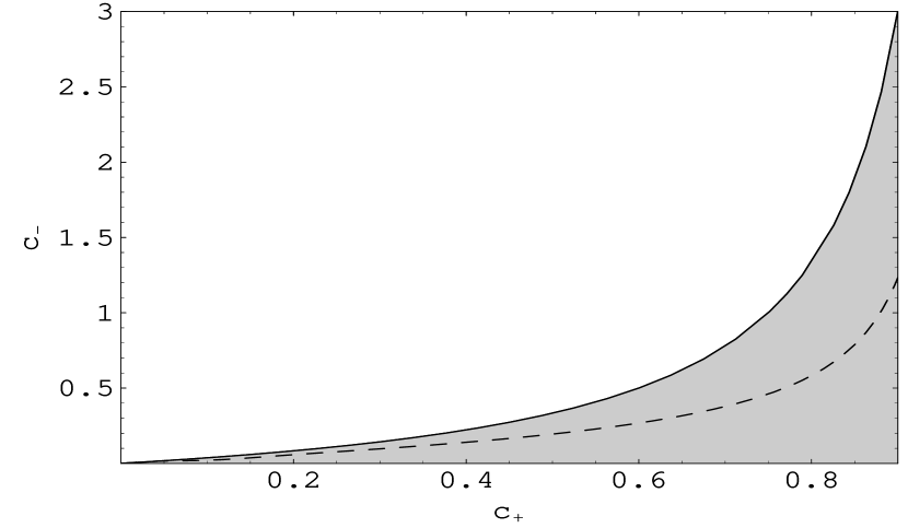
Figure 1: Class of allowed ae-theories, if strong field effects in binary pulsar systems can be ignored. The four-dimensional $c_{n}$ space has been restricted to the $(c_{+},c_{-})$ plane by setting the PPN parameters $\alpha_{1}$ and $\alpha_{2}$ to zero via the conditions (114). The shaded region is the region allowed by collected non-binary constraints, demarcated in (115). The dashed curve is the curve along which binary pulsar tests will be satisfied, assuming ae-theory weak field expressions. Along both this curve and the boundary of the allowed region, $c_{-}\rightarrow\infty$ as $c_{+}\rightarrow 1$. The curve remains within the allowed region for all $c_{+}$ between 0 and 1. Strong field effects may lead to system-dependent corrections to the binary pulsar curve for large $c_{n}$; however, all such curves will coincide with the weak field curve for $|c_{n}|\lesssim(0.01)$ given current observational uncertainties Foster (2006a).

Observational error allows this curve to be widened into a band. As explained in the Introduction, the standard method of measuring radiation damping is to observe the rate of change of orbital period $\dot{P}$ of a binary system Will (2001); Stairs (2003), which will be proportional to $\dot{\mathcal{E}}$. The smallest relative observational uncertainty in $\dot{P}$, which equates with the relative uncertainty in $\dot{\mathcal{E}}$, is of order $0.1\%$ for the Hulse-Taylor binary B1913+16 Will (2001); Stairs (2003). This uncertainty permits the band $|\mathcal{A}-1|\lesssim 10^{-3}$. Numerical results indicate that at least for small $c_{\pm}$, this band corresponds roughly to $c_{\pm}$ within about $10^{-3}$ of the $\mathcal{A}=1$ curve.