Time, clocks, parametric invariance and the Pioneer Anomaly v2

Abstract

In the context of a parametric theory (with the time being a dynamical variable) we consider the coupling between the quantum vacuum and the background gravitation that pervades the universe (unavoidable because of the universality of gravity). In our model the fourth Heisenberg relation introduces a possible source of discrepancy between the marches of atomic and gravitational clocks, which accelerate with respect to one another. This produces another discrepancy between the observations, performed with atomic time, and the theoretical analysis, which uses parametric astronomical time. Curiously, this approach turns out to be compatible with current physics; lacking a unified theory of quantum physics and gravitation, it cannot be discarded a priori. It turns out that this phenomenon has the same footprint as the Pioneer Anomaly, what suggests a solution to this riddle. This is because the velocity of the Pioneer spaceship with respect to atomic time turns out to be slightly smaller that with astronomical time, so that that the apparent trajectory lags behind the real one. In 1998, after many unsuccessful efforts to account for this phenomenon, the discoverers suggested “the possibility that the origin of the anomalous signal is new physics”.

1 Introduction

The problem of time is one of the most obscure and controversial in the history of knowledge, and has obvious implications in all the fields of thought. Sticking to physics, the problem is initially posed in the dynamical description of the systems (i. e. equations of motion). In this regard, the starting point is the a priori existence of a parameter $t$, called from now onwards “parametric time”, which describes the Newtonian concept of time. It is a fundamental part of a structure of reality constituted by an inert background in which dynamics takes place, but which, paradoxically, lacks on its turn of a dynamic character.

It must be emphasized that the equations of physics do not contain magnitudes in themselves but rather their measurements. It is thus more in the scope of physics to speak about “clocks” or “clock-time” than about time. In more intuitive terms, the problem can be posed as a question on the dynamical character or not of the time variable (parametric and deparametrized theories).

Traditionally, quantum physics has stated that the sea of virtual pairs that pop-up and disappear constantly in empty space, i. e. the quantum vacuum, has infinite energy density as follows from the simple application of its basic principles. However, there is now some evidence that it may be finite. In fact, it is not understood why this density seems to be so small as is shown by its possible cosmological manifestations. The question is important since the quantum vacuum fixes the values of some observable quantities, as the electron charge and the light speed, or gives rise to observable phenomena such as the Casimir effect or the Lamb shift.

The plan of this paper is as follows. Section 2 is devoted to discuss the inclusion of a dynamical time in Hamiltonian formalism. It is shown in section 3 that a coupling between the background gravitation that pervades the universe and the quantum vacuum is unavoidable, and that this determines that atomic clocks must march differently from the astronomical ones. In section 4, we look for an observable effect of this coupling, the best candidate being the so-called Pioneer anomaly. Section 5 shows that the coupling is not in conflict with astronomical data. Finally in section 6 we state our conclusions.

2 Time and clocks

In classical dynamics the physical time appears as a non-dynamical variable that allows the expression of the action integral with the form $S=\int L{\rm d}t$. As a consequence of this non-dynamical character, does not exist a canonical momentum conjugate to $t$. From the Hamiltonian

$$H(p,q)=\sum p\,\dot{q}-L\,,$$ (1)

the equations of motion in the standard form are $\dot{q}=\partial H/\partial p$, $\dot{p}=-\partial H/\partial q$. To translate this formal machinery to a scheme in which time acquires the character of a dynamical variable, there exists a canonical approach which allows an interpretation in terms of “clock-time” with its specific dynamical variables [1, 2, 3]. Instead of the deparametrized action $S=\int[p\,\dot{q}-H(p,q)]{\rm d}t$, we can use the alternative form

$$S=\int\{\Pi(t)\dot{\sigma}(t)+p\,(t)\dot{q}(t)-u(t)[\Pi(t)+H(p\,(t),q(t))]\}{\rm d}t\,,$$ (2)

(overdot means derivation with respect to the parameter $t$) where $H(p\,(t),q(t))$ has the same functional form as the Hamiltonian in (1), $t$ is introduced in such a way that the theory becomes invariant with respect to reparametrizations and $\sigma(t),\,\Pi(t)$ are conjugate dynamical variables that describe the clock. Note that $\Pi_{u}$, the momentum conjugate to $u(t)$, weakly vanishes.

The corresponding Hamiltonian writes

$$\hat{H}=u[\Pi+H(p,q)]+\lambda\,\Pi_{u}\,,$$ (3)

where $\lambda$ is a Lagrangian multiplier. The stability of the weak condition $\Pi_{u}=0$ implies $\Pi+H(p,q)=0$. Both are first-class constraints (i. e. symmetries). The transformations induced by $\Pi_{u}$ allow then to interpret $u(t)$ as an arbitrary function which can be considered as non-dynamical. The extended Hamiltonian is then

$$H^{E}=u[\Pi+H(p,q)]\,,$$ (4)

being hence singular as far as it is proportional to the scalar constraint. Simple algebra allows to verify that $\Pi+H(p,q)$ is the reparametrization generator, as requested by the invariance properties of the action (2). The equations of motion are then

$$\dot{q}={\partial H^{E}\over\partial p}=u{\partial H\over\partial p}\,;\quad\dot{p}=-{\partial H^{E}\over\partial q}=-u{\partial H\over\partial q}\,;\quad u=\dot{\sigma}\,;\quad\dot{\Pi}=-\dot{H}=0\,.$$ (5)

From these equations it follows that

$${{\rm d}q\over{\rm d}\sigma}={\partial H\over\partial p}\,;\quad{{\rm d}p\over{\rm d}\sigma}=-{\partial H\over\partial q}\,;\quad u={{\rm d}\sigma\over{\rm d}t}\,;\quad{{\rm d}H\over{\rm d}\sigma}=0\,.$$ (6)

The first two are the canonical equations of motion with $\sigma$ as the time variable. The third one expresses what we call the “march” of the clock $u$ with respect to the parameter $t$. This theory being invariant under reparametrization, we may fix the gauge by the condition $\sigma=t$ (i. e. $u=1$), so that we recover the ordinary canonical formalism with $t$ being the Newtonian time. We see that with this choice $\sigma$ is the time measured by an ideal clock, defined as one which can be made to run with the Newtonian time. As $\sigma$ and $\Pi$ (which is weakly equal to $-H$) are canonically conjugate variables, the fourth Heisenberg relation (involving now a dynamical time variable and the energy) acquires clearly a dynamical meaning. Notice the close analogy between the third equation (6) with the very concept of proper time in general relativity ${\rm d}\tau=\sqrt{g_{00}}\,{\rm d}t$, where $\sqrt{g_{00}}$ is the march of a proper clock with respect to the parametric time. It must be emphasized that the ordinary deparametrized dynamics is a particular gauge of this scheme. The extension of this formalism to more complex functional dependence on the time variables gives essentially the same result, although at the expense of some unnecessary complexity [1]. Note that this formulation gives a dynamical basis for the fourth Heisenberg relation because the energy and the time $\sigma$ are clearly conjugate dynamical variables with Poisson bracket $[H,\sigma]=1$. This precision will be important later.

As a matter of fact, no criterion exists, other than an arbitrary choice, to fix the march of a real clock to that of parametric time, being this one essentially unobservable by its own definition, in a parametric invariant description. The Hamiltonian (3) is the sum of two terms, describing, respectively, the physical system and the clock. The equation of motion of the second term, $H_{\rm clock}=u\Pi+\lambda\Pi_{u}$, is precisely that of a clock $u={\rm d}\sigma/{\rm d}t$. The situation has to be understood as the arbitrary definition of standard clock as one that verifies the relationship $u={\rm d}\sigma_{0}/{\rm d}t=1$, denoting the time of the standard clock as $\sigma_{0}$. Notice that the definition of a standard clock refers precisely to its march. No change of units is involved as it happens when scale transformations are present [4].

The simplest example of a theory with a clock is given by the free particle in special relativity, described by the action

$$S=-mc\int{\rm d}s\equiv-mc\int\sqrt{\dot{x}_{0}^{2}-\dot{x}_{i}^{2}}\,{\rm d}t\,,$$

which is parametric invariant by construction. The corresponding scalar constraint leads us to the on-shell condition $p_{0}^{2}-p_{i}^{2}=m^{2}c^{2}$.

The extended hamiltonian analogous to (4) reads

$$H^{E}=u[p_{0}+H]\,,\qquad\left(H=\mp\sqrt{p_{i}^{2}+m^{2}c^{2}}\right)\,,$$

showing the role as a clock played by the dynamical variable $x_{0}$. The result is essentially the same in the presence of a non-euclidian metric, both are examples of a class of theories having a clock as well as parametric invariance. The Einstein-Hilbert action for pure gravity, quite on the contrary, is a parametric invariant theory without any clock as a dynamical variable. This is a situation that is by no means obvious to understand.

As long as the observations make use of only the standard clock, the scheme is nothing else than the Hamiltonian equations. This may not occur, however, if there is another clock with a different march. In the latter case, the motion equations are (6), but with $\sigma_{0}$ instead of $t$

$${{\rm d}q\over{\rm d}\sigma}={\partial H\over\partial p}\,;\qquad{{\rm d}p\over{\rm d}\sigma}=-{\partial H\over\partial q}\,;\qquad{{\rm d}\sigma\over{\rm d}\sigma_{0}}=u\,,$$ (7)

which describe the physics of a system in operationally realistic terms. This means that they do not refer to any unobservable parametric time but to $\sigma_{0}$ and $\sigma$, which are times really observed by real clocks. The novelty is here the presence of the third equation (7), which is the dynamic equation of the second clock with respect to the standard one.

It must be underscored that there is no criterion to determine the march $u$, other that to refer to the internal properties of the clock or the pure observation, particularly if they are based on different phenomena. Physics has accepted traditionally without any discussion the implicit “principle” that all kinds of clocks have the same march and measure the same time. However, if two clocks are based on different phenomena, they are not necessarily equivalent, specially in the case where the parametric invariance is broken, in the sense that the march ${\rm d}\sigma/{\rm d}\sigma_{0}$ may not be a constant (if it were, the two clocks would measure the same time with different units). In the following, we will use as standard clock-time $t_{\rm atomic}$, i. e. the time measured by the atomic clocks

3 Coupling between the background gravitation and the quantum vacuum

Following the same scheme as in section 2, we assume here a classical parametric invariant description, which allows us to choose $t$ as a non-relativistic Newtonian time. Let us consider the background gravitational potential that pervades the universe and let us do it from a phenomenological viewpoint. The potential near Earth can be written approximately as $\Psi_{\rm E}({\bf r},t)=\Psi_{\rm loc}({\bf r})+\Psi(t)$ (here $\Psi=\Phi/c^{2}$, $\Phi$ being the dimensional Newtonian potential). The first term $\Psi_{\rm loc}$ is the part of the local inhomogeneities, as the Sun and the Milky Way, which are not expanding so that it is time independent. The second $\Psi(t)$ is due to all the mass-energy in the universe assuming that it is uniformly distributed. Contrary to the first, it depends on time because of the expansion. The former has a nonvanishing gradient but is small, the latter is larger but its gradient vanishes. In the following $\Psi(t)$ will be called the background potential of the entire universe. Since the gravity is weak and the geometry of the universe has approximately flat space sections, we take the Newtonian approximation.

Because gravitation is a long range universal interaction that affects to all the matter and energy in the universe, there must be necessarily a coupling between the background potential $\Psi(t)$ and the quantum vacuum. Consequently, the existence must be admitted of some kind of adiabatic progressive modification of the structure of the quantum vacuum in the expanding universe. The analysis of the previous section shows that the dynamical time and the energy can be defined as conjugate canonical variables, what gives a dynamical basis to the fourth Heisenberg relation $\Delta E\cdot\Delta\tau\approx\hbar$. Let us consider now the sea of virtual pairs in the quantum vacuum, with their charges and spins, assuming that its energy density is finite. On the average and phenomenologically, a virtual pair created with energy $E$ lives during a time $\tau_{0}=\hbar/E$, according to the fourth Heisenberg relation. This has an important consequence: the optical density of empty space must depend on the gravitational field. Indeed, at a spacetime point with gravitational potential $\Psi({\bf r},t)$ , the pairs have an extra energy $E\Psi$, so that their lifetime must be $\tau_{\Psi}=\hbar/(E+E\Psi)=\tau_{0}/(1+\Psi).$

The conclusion seems clear [5, 6]: the number density of pairs $\cal N$ depends on $\Psi$ as ${\cal N}_{\Psi}={\cal N}_{0}/(1+\Psi)$. If $\Psi$ decreases, the quantum vacuum becomes denser, since the density of charges and spins becomes higher; if $\Psi$ increases, it becomes thinner. Consequently, the gravity created by mass or energy thickens the quantum vacuum, while the gravity created by the cosmological constant or the dark energy attenuates it. This is important, since the quantum vacuum plays a decisive role to renormalize the naked or bare values of some quantities to their observed values, as is the case of the electron charge and the light speed. It must be stressed that this is not an ad hoc hypothesis, but a necessary consequence of the fourth Heisenberg relation and the universality of gravitation. The effect of the time independent $\Psi_{\rm loc}$ is neglected here because, as will be shown, the potential acts in this model through its time derivative.

We accept then the following phenomenological hypothesis: the quantum vacuum can be considered as a substratum, a transparent optical medium characterized by a relative permittivity $\varepsilon_{\rm r}(\Psi)$ and a relative permeability $\mu_{\rm r}(\Psi)$, which are decreasing functions of $\Psi(t)$. As $\Psi(t)$ increases, the optical density of the medium decreases (since there are less charges and spins) and vice versa. Therefore, the permittivity and the permeability of empty space can be written as $\varepsilon=\varepsilon_{\rm r}\varepsilon_{0}$ and $\mu=\mu_{\rm r}\mu_{0}$, where the first factors express the effect of the gravitational potential, i. e., the thickening or thinning of empty space. We can write, at first order in the variation of $\Psi(t)$,

$$\varepsilon_{\rm r}(t)=1-\beta[\Psi(t)-\Psi(t_{0})],\qquad\mu_{\rm r}(t)=1-\gamma[\Psi(t)-\Psi(t_{0})]\,,$$ (8)

where $\Psi(t_{0})$ is the reference potential at present time $t_{0}$ and $\beta$ and $\gamma$ are certain coefficients, necessarily positive since the quantum vacuum must be dielectric but paramagnetic (its effect on the magnetic field is due to the magnetic moments of the virtual pairs). The results of this paper will depend only on the semisum $\eta=(\beta+\gamma)/2$. Not surprisingly, it turns out that $\Psi(t)$ varies adiabatically (because of the expansion) and that its time derivative at present time $\dot{\Psi}_{0}=\dot{\Psi}(t_{0})$ is positive and very small, of the order of $H_{0}$ as we will see later. It must be underscored that eqs. (8) express a modification of the structure of the quantum vacuum as an effect of its coupling with the background gravitation in the expanding universe.

It is easy to show that if $\varepsilon_{\rm r}$ and $\mu_{\rm r}$ decrease adiabatically as (8) (and the optical density of empty space, therefore), the frequency and the speed of an electromagnetic wave increase adiabatically as

$$\dot{\nu}/\nu=\dot{c}/c=-(\dot{\varepsilon}/\varepsilon+\dot{\mu}/\mu)/2=\eta\dot{\Psi}_{0}\,,$$ (9)

or, equivalently,

$$\nu=\nu_{0}[1+\eta\dot{\Psi}_{0}(t-t_{0})]\,,\qquad c=c_{0}[1+\eta\dot{\Psi}_{0}(t-t_{0})]\,.$$ (10)

The proof is very simple [5, 7]: just write the Maxwell’s equations with $\varepsilon$ and $\mu$ decreasing adiabatically with time as in (8) to find that eqs. (9) and (10) are satisfied at first order in $\dot{\Psi}_{0}$. If $\varepsilon,\,\mu$ vary with time as an effect of the change of the densities of virtual charges and spins, the speed of light changes also. This is not dissimilar to what happens to light in a medium, say diamond, where speed is different from $c$ because the quantum effects of the lattice add to those of empty space.

As a consequence, the quantum vacuum can be characterized by a refractive index $n(t)=1+\eta\dot{\Psi}_{0}(t-t_{0})$ depending on the Newtonian time. We can interpret this result in two ways: (i) the first and obvious one is that light accelerates with the Newtonian time; however, attention must be paid to the fact that this statement depends on the particular choice of the Newtonian clock, as was shown before. (ii) Nevertheless, since the dynamical equation of a clock is its march, it suffices to take a clock with march relative to the Newtonian one equal to the refractive index

$${{\rm d}\sigma\over{\rm dt}}=n(t)\,,$$ (11)

for the frequencies and the speed of light to be constant (10). It is clear that such a clock is precisely an atomic clock since the periods of an electromagnetic wave are its basic units.

As we said before, there is no clock in Einstein-Hilbert formulation of General Relativity. However, the constancy of the light speed provides us with a dynamical time: the proper time. In fact the geometric structure of space-time induces a relative permittivity $\varepsilon_{\rm r}$ and permeability $\mu_{\rm r}$ of empty space different from 1, their common value being $\varepsilon_{\rm r}=\mu_{\rm r}=(g_{00})^{1/2}$ [8]. As a consequence of diff-invariance, the use of the proper time defined as ${\rm d}\tau=\sqrt{g_{00}}\,{\rm d}t$ restores the constancy of the light speed.

Being a quantum effect, the coupling to the quantum vacuum breaks diff-invariance and cannot, therefore, be included in the definition of proper time. Consequently, it is an alien element that must be added to general relativity.

Hence, three times must be considered. They are

(i) the parametric time $t$, namely the ephemerids time (which is a coordinate time), used to calculate the trajectory of the spaceships.

(ii) The proper time $\tau$ of General Relativity.

(iii) The time of the atomic clocks $t_{\rm atomic}$, defined as

$${\rm d}t_{\rm atomic}=[1+\eta(\Psi(t)-\Psi(t_{0})]\,{\rm d}\tau=[1+\Psi_{\rm loc}+\eta(\Psi(t)-\Psi(t_{0})]\,{\rm d}t\,.$$ (12)

We will omit in the following the term $\Psi_{\rm loc}$ because it is constant and we will be concerned with the time variation of the potential.

It is usually assumed that the two dynamical times $\tau$ and $t_{\rm atomic}$ are in fact the same one. However, this is no longer true if $\eta\neq 0$.

4 Looking for the effect

4.1 The Pioneer anomaly

Anderson et al. reported in 1998 a curious anomalous effect [9, 10]. It consists in an adiabatic frequency blue drift of the two-way radio signals from the Pioneer 10/11 (launched in 1972 and 1973), manifest in a residual Doppler shift, which increases linearly with time as

$$\dot{\nu}/\nu=2a_{\rm t}\,,\quad\mbox{or}\quad\nu=\nu_{0}\,[1+2a_{\rm t}(t-t_{0})]\,,$$ (13)

where $t_{0}$ is the launch time, $a_{\rm t}=(1.27\pm 0.19)H_{0}$ and $H_{0}$ is the Hubble constant (overdot means time derivative). More than 30 years afterwards, the phenomenon is still unexplained. Since it was detected as a Doppler shift that does not correspond to any known motion of the ships, its simplest interpretation is that there is an anomalous constant acceleration towards the Sun. However, this is not acceptable since it would conflict with the well known ephemeris of the planets and with the equivalence principle.

Anderson attempted a second interpretation: $a_{\rm t}$ would be “a clock acceleration”, expressing a kind of inhomogeneity of time. They imagined it in an intuitive and phenomenological way, without any theoretical foundation, saying that, in order to fit the trajectory, “we were motivated to try to think of any (purely phenomenological) ‘time’ distortions that might fortuitously fit the Pioneer results” (our emphasis, ref. 2, section XI). They obtain in this way the best fits to the trajectory (using the adjective “fascinating”). In one of them, which they call “Quadratic time augmentation model”, they add to the TAI-ET (International Atomic Time-Ephemeris Time) transformation the following distortion of ET

$$\mbox{ET}\rightarrow\mbox{ET}^{\prime}=\mbox{ET}+{1\over 2}\,a_{\rm ET}\,\mbox{ET}^{2}\,.$$ (14)

This means to take a new time ET^′ that is a quadratic function of ET and which, therefore, accelerates with respect to ET. Note that ET is a parametric coordinate time while TAI is a dynamical time. But they gave up the idea because of the lack of any theoretical foundation and contradictions with the determination process of the orbits. They were not on the back track, however, as will be seen here.

In 1998, after many unsuccessful efforts to account for it, the discoverers suggested “that the origin of the anomalous signal is new physics” [9]. In other words, to try non-standard ideas could be a good strategy to solve the riddle, specially if they are not in conflict with current physics, as is the case with the proposals of this work.

4.2 A problem of dynamics of time

From now on, the ephemeris time will be called “astronomical time” and noted $t_{\rm astr}$. It turns out, as will be shown, that the anomaly has the same observational signature as an acceleration of the marches of atomic and the astronomical clocks with respect to one another. In other words, as the deceleration of the astronomical clocks with respect to the atomic clocks (or, equivalently, to the acceleration of the latter with respect to the former). This might seem surprising since it is always assumed as a matter of fact that both types of clocks measure the same time. This is not necessarily true, however, since they are based on different physical laws. The importance of this point must be stressed. The astronomical clock-time, say $t_{\rm astr}$, is defined by the trajectories of the planets and other celestial bodies. It is measured with classical and gravitational clocks, the solar system for instance. On the other hand, the atomic clock-time, say $t_{\rm atomic}$, is founded on the oscillations of atomic systems. It is measured using quantum and electromagnetic systems as clocks, in particular the oscillations of atoms or masers. Note that, contrary to the concept of time, which is subtle and difficult, the idea of “clock” is clearly defined from the operational point of view. This is done by means of certain dynamical systems, the clocks, in such a way that the time measured by each one is a dynamical variable, the angular position of a pointer for instance. The measured time could be different from one clock to the other since, at least in principle, they could tick at different rates, even at the same place and having the same velocity. Indeed, eq. (13) can be understood as a progressive decrease of the period of the radio signal, so that the basic unit of the atomic clock-time would be decreasing with respect to the astronomical time of the orbit.

It is clear that the two clock-times are very close at least but, since we lack a unified theory of gravitation and quantum physics, the assumption that they are exactly the same $t_{\rm astr}=t_{\rm atomic}$ must not be taken for granted. In the explanation proposed here, the two times are different because of the previously discussed coupling between the quantum vacuum and the background gravitation, in such a way that $a_{\rm t}={\rm d}^{2}t_{\rm atomic}/{\rm d}t_{\rm astr}^{2}$, which gives a precise meaning to what Anderson et al. called “clock acceleration”: it is the acceleration of the time of the quantum atomic clocks with respect to the astronomical time, this one determined by purely gravitational and classical phenomena. In such a way, the Pioneer becomes a two-clock system: the astronomical clock of the orbit and the atomic clock that measures the time of the devices used to track the trajectory, which are based on quantum physics. The ideas expounded here follow from the confluence of two research lines, one on the Pioneer Anomaly itself [5, 6, 7], the other on the dynamics of time [1, 2].

4.3 The deceleration of the astronomical clocks

As already said, eq. (13) suggests that the periods of the microwaves from the Pioneer are decreasing with respect to the time used to define the orbit; in other words, that the atomic clocks accelerates with respect to the astronomical clock. Eqs. (9)-(10) show that something similar happens as a consequence of the coupling between quantum vacuum and gravitation, if $\dot{\Psi}_{0}>0$. More precisely that the frequencies and the light speed increase if defined with respect to $t_{\rm astr}$. However, using instead the time $t_{\rm atomic}$, defined through

$${\rm d}t_{\rm atomic}=[1+\eta\dot{\Psi}_{0}\,(t_{\rm astr}-t_{\rm astr,\,0})]\,{\rm d}t_{\rm astr}\,,\;\;\mbox{so that}\;\;\left.{{\rm d}^{2}t_{\rm atomic}\over{\rm d}t_{\rm astr}^{2}}\,\right|_{0}=\eta\dot{\Psi}_{0}=a_{\rm t}$$ (15)

there is no anomaly, since both the frequency and the light speed are then constant with this time. It is clear that $t_{\rm atomic}$ is the time measured by the atomic clocks, since the periods of the atomic oscillations, which are decreasing if measured with the astronomical time (as shown by (9) where $t=t_{\rm astr}$), are obviously constant with respect to $t_{\rm atomic}$ itself, in fact they are its basic units. The meaning of $a_{\rm t}$ is neat also: it is the acceleration of the atomic clock-time with respect to the astronomical clock-time (note that it would be zero without the quantum vacuum, since $\eta=0$ then). Alternatively, it could be said that $-a_{\rm t}$ is the deceleration of the march of the astronomical clock-time with respect to the atomic clock-time. It follows then from (15) and (13) that what Anderson et al. observed could well be the march of the atomic clocks that tracked the ship with respect to the astronomical clock of its orbit $u=1+\eta\dot{\Psi}_{0}\,(t_{\rm astr}-t_{\rm astr,\,0})$. After synchronizing the two so that they give the same time now, $t_{\rm astr,\,0}=t_{\rm atomic,\,0}=0$, eqs. (15) can be written in the two equivalent ways

$$t_{\rm atomic}=t_{\rm astr}+{1\over 2}\,\eta\dot{\Psi}_{0}\,t_{\rm astr}^{2},\quad t_{\rm astr}=t_{\rm atomic}-{1\over 2}\,\eta\dot{\Psi}_{0}\,t_{\rm atomic}^{2}\,,$$ (16)

near present time. The first coincides with eq. (14) if $t_{\rm astr}=\mbox{ET}$ and $t_{\rm atomic}=\mbox{ET}^{\prime}$. The importance of this equation must be stressed since it explains why Anderson et al. obtained good fits by distorting phenomenologically the time.

All this shows (eqs. (9)-(10)) that the effect of the quantum vacuum would be to accelerate adiabatically the light and to increase progressively the frequencies if they are measured with the astronomical time $t_{\rm astr}$. However they are constant if measured with the atomic time $t_{\rm atomic}$. Synchronizing these two times and taking the international second as their common basic unit at present time, then ${\rm d}t_{\rm astr}={\rm d}t_{\rm atomic}$ (ref. 5). This means that we can keep the same symbol for the two derivatives ${\rm d}\Psi/{\rm d}t_{\rm astr}={\rm d}\Psi/{\rm d}t_{\rm atomic}=\dot{\Psi}_{0}$ at present time.

If the march $u={\rm d}t_{\rm atomic}/{\rm d}t_{\rm astr}=1+\eta\dot{\Psi}_{0}\,(t_{\rm astr}-t_{\rm astr,\,0})$ is not constant, the speed measured with Doppler effect and devices sensible to the quantum time, say $v_{\rm atomic}={\rm d}\ell/{\rm d}t_{\rm atomic}$, would be different from the astronomical speed $v_{\rm astr}={\rm d}\ell/{\rm d}t_{\rm astr}$. In the case of the Pioneer anomaly, $u>1$ (because $t_{\rm astr}>t_{\rm 0,\,astr}$), so that

$$v_{\rm atomic}=v_{\rm astr}\,{{\rm d}t/{\rm d}t_{\rm atomic}}=v_{\rm astr}[1-a(t_{\rm astr}-t_{\rm astr,\,0})]<v_{\rm astr}\,.$$ (17)

Since the gravitation theory gives $v_{\rm astr}$ while the observers measure $v_{\rm atomic}$, there must be a discrepancy between theory and observation. An apparent but unreal violation of standard gravity would be detected.

4.4 Explanation of the anomaly

These arguments give a compelling explanation of the anomaly as an effect of the discrepancy between these two times. Let us see why. The frequencies measured by Anderson et al. are standard frequencies defined with respect to atomic time $t_{\rm atomic}$, since they used devices based on quantum physics. They did not measure frequencies with respect to the astronomical time. However, since (i) the trajectory is determined by standard gravitation theories with respect to astronomical time and (ii) the observation used atomic time, they found a discrepancy with their expectations: this is the Pioneer Anomaly.

To be specific, the discrepancy consists in the following. The distance travelled by a ship along a given trajectory can be expressed in two ways

$$d=\int_{0}^{t_{\rm atomic}}\!\!\!\!\!\!\!\!v_{\rm atomic}(t^{\prime}){\rm d}t^{\prime}=\int_{0}^{t_{\rm astr}}\!\!\!\!\!v_{\rm astr}(t^{\prime}){\rm d}t^{\prime}\,,$$ (18)

where $t^{\prime}=t_{\rm atomic}$ in the first integral, $t^{\prime}=t_{\rm astr}$ in the second and $(0,t_{\rm atomic})$ and $(0,t_{\rm astr})$ are the same time interval expressed with the two times (because $v_{\rm atomic}=v_{\rm astr}/u$ and ${\rm d}t_{\rm atomic}=u{\rm d}t_{\rm astr}$). Equation (18) is always valid, if the two times are equal and if they are different as well. What we are proposing as the solution to the riddle is that the two times are in fact different. If, however, they are assumed to be equal $t_{\rm astr}=t_{\rm atomic}$, then the distance deduced from observations $d_{\rm observ}$ and the expected distance according to standard gravitation theory $d_{\rm theory}$ up to the same $t_{\rm atomic}$, which are

$$d_{\rm observ} = \int_{0}^{t_{\rm atomic}}\!\!\!\!\!\!\!\!\!\!\!\!v_{\rm atomic}(t^{\prime})dt^{\prime}\,,\quad d_{\rm theory}=\int_{0}^{t_{\rm atomic}}\!\!\!\!\!\!\!\!\!v_{\rm astr}(t^{\prime}){\rm d}t^{\prime}\,,$$

with $t^{\prime}=t_{\rm atomic}$ in both integrals, would be different. Now, if $u>1$ as during the Pioneer flight, the atomic velocity is smaller so that $d_{\rm observ}<d_{\rm theory}$: it would seem that the ship runs through a smaller than expected distance. Apparently, it would lag behind the expected position.

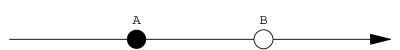
Figure 1: Schematic representation with arbitrary units of the Pioneer anomaly (explanation in the text.)

All this is explained in Figure 1, where the Pioneer trajectory receding from the Sun is plotted schematically. The spacecraft moves in the sense of the arrow. The white circle at $B$ is the position of the ship according to standard gravitation, its real position in fact if this theory is correct. The black circle at $A$ is the apparent position, deduced from the the ship velocity after measuring with atomic clocks and devices the Doppler effect on the frequencies of the signals. If the two times were the same, as usually assumed, $A$ and $B$ would coincide; if they are not, as in this model, $A$ and $B$ separate and $A$ would be an apparent position only. In the latter case, which one of the pair $A,\,B$ moves faster depends on the value of the relative march of the atomic clocks with respect to the astronomical clocks $u={\rm d}t_{\rm atomic}/{\rm d}t_{\rm astr}$.

Since in any time interval during the flight of the ship ${\rm d}t<{\rm d}t_{\rm atomic}$, the speed measured with Doppler effect and devices sensible to the quantum time, $v_{\rm atomic}$, must be smaller than the astronomical speed $v_{\rm astr}$. There would be an unexplained Doppler residual, easily interpretable as an anomalous acceleration towards the Sun. Indeed, in the case of one way signals, $v_{\rm atomic}=v_{\rm astr}{{\rm d}t/{\rm d}t_{\rm atomic}}={v_{\rm astr}/u}=v_{\rm astr}/[1+\eta\,\dot{\Psi}_{0}(t-t_{0})]$ while for two-way signals

$$v_{\rm atomic}=v_{\rm astr}/u^{2}=v_{\rm astr}[1-2\eta\dot{\Psi}_{0}(t-t_{0})]<v_{\rm astr}\,,$$ (20)

at first order. In other words, the ship would seem to recede from the Sun more slowly than expected. There would be an extra blueshift, since the failure to include the acceleration ${\rm d}^{2}t_{\rm atomic}/{\rm d}t_{\rm astr}^{2}$ in the analysis mimics a blue Doppler residual $\dot{\nu}/\nu=2\eta\,\dot{\Psi}_{0}$ or $\nu=\nu_{0}[1+2\eta\dot{\Psi}_{0}(t-t_{0})]$ (compare with (13)). This is precisely what Anderson et al. observed and gives the right result if $\eta\dot{\Psi}_{0}\simeq 1.3H_{0}$.

The preceding arguments explain the statement made at the beginning of section 2 that the Pioneer anomaly has the same observational footprint as an acceleration of the atomic clock-time with respect to the astronomical time (or as a deceleration of the latter with respect to the former, what is the same).

For this model to be right, it is necessary that $\dot{\Psi}_{0}>0$, i.e. that the present value of the time derivative of the background potential be positive. It could be argued that this can be considered in fact a prediction of the model. Alternatively, a simple argument shows that $\Psi(t)$ is increasing now. The potential $\Psi$ can be taken to be the sum of two terms, one due to the matter, either ordinary and dark, and another to the cosmological constant or the dark energy. The first is negative and increases with time because the galaxies are separating; the second is positive and increases with the radius of the universe. Indeed their values are proportional to $-1/S$ and $+S^{2}$, respectively, where $S$ is the scale factor. This can be further elaborated with a simple model of $\Psi$, in which $\dot{\Psi}_{0}$ is positive and of order $H_{0}$ (see [7]).

5 Agreement with the gravitational redshift and other observations

The coupling background gravity-quantum vacuum affects the astronomical time but does not change the atomic time. For this reason, this model predicts the same standard values for the frequencies of all the spectral lines because it does not affect the measurements made with atomic clock-time. Any one of these lines, for instance the 1,420 MHz line of the hyperfine structure of Hydrogen, known with an accuracy of $10^{-14}$, has in this model exactly the same value as in the tables of physical constants or data. The reason is simple: this frequency is calculated in atomic theory and measured with devices based on quantum physics, which use therefore the atomic time $t_{\rm atomic}$, not the astronomical time $t_{\rm astr}$. These include lasers, masers, transponders, prisms, diffraction gratings or spectrographs. What is new in this work is that the frequencies defined with respect to $t_{\rm astr}$ are different but these are not usually measured, probably never.

This model obviously complies with the experiments on gravitational redshift, because they are performed with atomic clocks, which are exactly the same thing in this work as in standard physics. In particular, it agrees with Einstein formula

$$\Delta\nu/\nu=-\Delta\Psi_{\rm loc}\,,$$ (21)

However, since the standard analysis is based on the equality of proper and atomic times, it can be clarifying to compare the two approaches. In this work and taking into account the local potential by means of ${\rm d}\tau=(1+\Psi_{\rm loc}){\rm d}t$, one has ${\rm d}t_{\rm atomic}=[1+\eta\dot{\Psi}_{0}(\tau-\tau_{0})]{\rm d}\tau$ at first order. The relative difference between the two approaches is therefore of order $\eta\dot{\Psi}_{0}\tau_{\rm flight}$, where $\tau_{\rm flight}$ is the flight time of the light beam. In the most precise observations by Levine and Vessot, with accuracy $\simeq 2\times 10^{-4}$, this time is $\simeq 3.3\times 10^{-2}\mbox{ s}$ [11]. The condition on the clock acceleration is then $a=\eta\dot{\Psi}_{0}<6\times 10^{-3}\mbox{ s}^{-1}$; $a$ is surely much smaller that this bound, probably of the order of $H_{0}$, otherwise the effect would have been detected before. The difference between $\tau$ and $t_{\rm atomic}$ is thus too small to de detected in experiments of this kind.

It might be argued that the deceleration of $t_{\rm astr}$ with respect to $t_{\rm atomic}$ predicted by this work would conflict with the well-known cartography of the Solar System, particularly with the observed periods of the planets. It is not so, however. The dominant potential, as indicated before, is that of the Milky Way, which can be taken as constant at the scale of the Solar System and equal to $\simeq 6\times 10^{-7}$. The march is then $u={\rm d}t_{\rm atomic}/{\rm d}t_{\rm astr}=1-6\times 10^{-7}$, which is constant. This means that the equations of the Solar System in Newtonian physics

$$\frac{{\rm d}^{2}{\bf r}_{i}}{{\rm d}t_{\rm astr}^{2}}=-\sum_{j\neq i}Gm_{j}\frac{({\bf r}_{j}-{\bf r}_{i})}{|{\bf r}_{j}-{\bf r}_{i}|^{3}}\,,$$ (22)

are the same with the two times $t_{\rm astr}$ and $t_{\rm atomic}$. The reason is clear: These equations are invariant under the transformation $t_{\rm astr}\rightarrow t_{\rm atomic}=u\,t_{\rm astr}$, $G\rightarrow G/u^{2}$ (they would not be invariant if $u$ is variable). The third Kepler law, for instance, is equally valid with $t_{\rm astr}$ and $G$ as with $t_{\rm atomic}$ and $G/u^{2}$. Indeed, the best value of $G$, obtained with atomic clocks, must be in fact $G/u^{2}$. There can be no conflict with the cartography of the Solar system.

6 Summary and conclusions

Our conclusions can be stated as follows.

(i) The natural framework to describe dynamics is a parametric invariant formulation including the time as a dynamical object (a clock-time). The equation of motion of a clock is precisely its march.

(ii) Because gravitation is long range and universal since it affects all kinds of mass or energy, a coupling must exist necessarily between the background gravitation that pervades the universe and the quantum vacuum. This coupling can be estimated from the fourth Heisenberg relation and implies a progressive attenuation of the quantum vacuum in the sense that the refractive index $n(t_{\rm astr})$ is a decreasing function of the astronomical time. However $n(t_{\rm atomic})=1$.

(iii) As argued before, the unexplained Pioneer anomaly (13) can be understood as the adiabatic decrease of the periods of the atomic oscillations with respect to the astronomical time. In other words, the solar system, considered as a clock, would run progressively slower than the atomic clocks. This would be an effect of the interaction between the background gravitational potential and the quantum vacuum and, therefore, a certain evidence of the interplay between gravitation and quantum physics. A consequence of this coupling would be an acceleration of the quantum clock-time of the atomic clocks $t_{\rm atomic}$ with respect to the classical astronomical clock-time $t_{\rm astr}$, equal to what Anderson et al. called the “clock acceleration”, $a_{\rm t}={{\rm d}^{2}t_{\rm atomic}/{\rm d}t_{\rm astr}^{2}}|\,_{0}>0$ (or, equivalently, there would be a deceleration of $t_{\rm astr}$ with respect to $t_{\rm atomic}$). The relation with the coupling background gravity-quantum vacuum is given as $a_{\rm t}=\eta\dot{\Psi}_{0}$, where $\dot{\Psi}_{0}$ is the present time derivative of the background potential and $\eta$ a coefficient that refers to the structure of the vacuum defined in section 3 (after equation (8)). In other words, we propose here that what Anderson et al. observed is the relative march of the atomic clock-time of the detectors with respect to the astronomical clock-time of the orbit $u={\rm d}t_{\rm atomic}/{\rm d}t_{\rm astr}=1+\eta\dot{\Psi}_{0}(t_{\rm astr}-t_{\rm astr,\,0})$ or, more precisely, its square $1+2\eta\dot{\Psi}_{0}(t_{\rm astr}-t_{\rm astr,\,0})$ because their signal was two-way (compare with (13)). Although this new idea may seem surprising and strange, it conflicts with no physical law or principle. In fact, it could be rejected only by using a theory embracing gravitation and quantum physics, which does not exists thus far.

(iv) The model here presented gives a qualitative explanation, at least, of the Pioneer anomaly, which could well be a manifestation of the mismatch between these two times, and a quantum gravity cosmological phenomenon therefore. In order to know whether this explanation can be also quantitative, it is necessary to estimate the value of the “clock acceleration” $a_{\rm t}$. However, this value depends on a coefficient, here called $\eta$, which cannot be calculated without a theory of quantum gravity. On the other hand, the Pioneer anomaly could be considered as a measurement of $a_{\rm t}$ to be used in the future as a test for quantum gravity. In any case, this explanation agrees with the experimental values of the spectral frequencies, the periods of the planets and the gravitational redshift.

Two final comments. First, as a consequence of the coupling between the background gravitation and the quantum vacuum, the light speed would increase with acceleration $a_{\ell}=a_{\rm t}c$ if defined or measured with respect to the astronomical clock-time. However it is constant if measured with the atomic clock-time. In fact, an atomic clock is the “natural clock” to define and measure the light speed, since its basic unit is the period of the corresponding electromagnetic wave, so that the speed and the frequencies are then necessarily constant. This means that $c$ is still a fundamental constant if measured with atomic time.

Second, since the Pioneer anomaly would be a quantum effect which causes the light speed and the frequency to increase if defined and measured with astronomical proper time, it would be alien to general relativity. It must be stressed also that, if we accept that there are non-equivalent clocks that accelerate with respect to one another because of a coupling between gravity and the quantum vacuum, a new field of unexplored physics opens, which includes the very idea of universal dimensional constant, in particular.

7 Acknowledgements.

We are grateful to J. Martín and R. Tresguerres for discussions. This work has been partially supported by a grant of the Spanish Ministerio de Educación y Ciencia.

References

- [1] Tiemblo A and Tresguerres R (2002) Internal Time and Gravity Theories Gen. Rel. Grav. 34 31-47
- [2] Barbero J F, Tiemblo A and Tresguerres R. (1998) Husain-Kuchar model: Time variables and nondegenerate metrics Phys. Rev. D 57, 6104-6112
- [3] Hanson A, Regge T and Teitelboim C Constrained Hamiltonian Systems (Accademia dei Lincei, Roma, 1976)
- [4] Canuto V, Adams P J, Hsieh S-H and Tsieng E (1977) Scale-covariant theory of gravitation and astrophysical applications Phys. Rev. 16 1643-1663.
- [5] Rañada A F (2003) The Pioneer riddle, the quantum vacuum and the variation of the light velocity Europhys. Lett. 63 653-659
- [6] Rañada A F (2003) The light speed and the interplay of the quantum vacuum, the gravitation of all the universe and the fourth Heisenberg relation Int J. Mod. Phys. D 12 1755-1762
- [7] Rañada A F (2004) The Pioneer anomaly as acceleration of the clocks Found. Phys. 34 1955-1971
- [8] L.D. Landau and E.M. Lifshitz, The Classical Theory of Fields (Pergamon Press, Oxford, 1975), chapter 10.
- [9] Anderson J D, Laing Ph A, Lau E L, Liu A S, Martin Nieto M and Turyshev S G (1998) Indication, from Pioneer 10/11, Galileo and Ulysses Data, of an Apparent Anomalous, Weak, Long-Range Acceleration Phys. Rev. Lett. 81 2858-2861
- [10] Anderson J D, Laing Ph A, Lau E L, Liu A S, Martin Nieto M and Turyshev S G (2002) Study of the anomalous acceleration of Pioneer 10 and 11 Phys. Rev. D 65 082004, 1-50
- [11] Will C, Theory and Experiment in Gravitational Physics (Cambridge University Press, Cambridge, 1993)