Brane-world Cosmology

Abstract

Brane-world models, where observers are restricted to a brane in a higher dimensional spacetime, offer a novel perspective on cosmology. I discuss some approaches to cosmology in extra dimensions and some interesting aspects of gravity and cosmology in brane-world models.

1 Cosmology after Einstein

A century after Einstein first proposed his theory of relativity, it has become a cornerstone of the physical sciences. Four dimensional spacetime provides the setting for describing physical processes and in particular provides the dynamical framework for cosmological models of our expanding Universe.

It was the general theory of relativity, proposed by Einstein in 1915, that for the first time provided equations with which to describe the dynamics of spacetime. Einstein’s equation

$$G_{AB}+\Lambda g_{AB}=8\pi G_{N}T_{AB}\,,$$ (1)

relates the intrinsic curvature, $G_{AB}$, of the metric, $g_{AB}$, to the local energy-momentum, $T_{AB}$, while allowing for the possibility of a non-zero cosmological constant, $\Lambda$. Consistency with Newtonian gravity in the weak-field, slow-motion limit is ensured by the appearance of Newton’s constant, $G_{N}$, in the constant of proportionality.

In much of modern cosmology Einstein’s tensor equation (1) conveniently reduces to the Friedmann constraint equation

$$3\left(H^{2}+\frac{K}{a^{2}}\right)=\Lambda+8\pi G_{N}\rho\,,$$ (2)

which relates the Hubble expansion, $H$, and spatial curvature $K/a^{2}$, of a homogeneous and isotropic Friedmann-Robertson-Walker (FRW) spacetime to the local energy density $\rho$.

Homogeneous and isotropic expansion has been used to build up a remarkably successful model for the evolution of our Universe starting with a hot Big Bang at a finite time in our past. This model has been tested not only by qualitative features such as the evolution of galaxy populations and the existence of a cosmic microwave background (CMB) radiation, but also quantitatively tested by comparing models of primordial nucleosynthesis with abundance of light elements.

One only needs to consider linear perturbations about a homogeneous and isotropic metric to build up a coherent picture of the formation of structure in our Universe. Small fluctuations, about one part in a hundred thousand, are observed in the temperature of the microwave background radiation and indicate the existence of small primordial perturbations in the distribution of matter and radiation in the early universe when the CMB last scattered, about 300,000 years after the Big Bang. These primordial density fluctuations provide the seeds around which the observed large-scale structure of our Universe can form simply by gravitational instability, in a cosmological model with appropriate contributions from radiation, baryonic matter, as well as cold dark matter and some form of dark energy, that behaves very much like Einstein’s cosmological constant today. A wealth of observational data now enables cosmologists to put this basic picture to the test and attempt to measure parameters such as the density of different forms of matter, the nature of the primordial perturbations, and Einstein’s gravitational laws.

At the same time fundamental questions remain unanswered. Why are there 3 large spatial dimensions (not 5 or 15)? why is the value of the cosmological constant so small? and what really happens at the initial Big Bang which represents a singular point at the start of our cosmological evolution? I cannot answer these questions in this talk, but I can show how brane-world models offer some novel and interesting perspectives on these issues. I should emphasize that this is a personal view and not intended to be a systematic review of all aspects of brane-world cosmology. For a more comprehensive review see Roy .

2 Extra dimensions

Superstring theory is an attempt to unify gravity with the other fundamental interactions in a self-consistent quantum theory, based on strings (extended 1-dimensional objects) as the fundamental constituents of matter rather than point particles. In particular string theory should be finite and singularity free.

For example, the existence of a minimal length scale in the effective theory leads to a “T-duality” that relates expanding and contracting cosmological solutions and has been proposed as the basis for the pre-Big Bang scenario GasVen that proposes a pre-Big Bang era preceding the hot Big Bang expansion. Unfortunately the nature of the transition from pre- to post-Big Bang is dependent on the nature higher-order, possibly non-perturbative, effects and remains elusive. This makes it hard to make robust predictions based on a pre-Big Bang phase.

It is not fair to say that string theory does not make any predictions. String theory does make a definite prediction for the number of spacetime dimensions. Spacetime should have 10 dimensions for a consistent, anomaly-free superstring theory GSW . This may not appear to be a huge success for the theory, but of we can only assert that there are four observable dimensions and it is quite possible that there exist extra dimensions that are very small and/or unobservable.

Only a few years after Einstein proposed his theory of dynamical four-dimensional spacetime, Kaluza began to consider the dynamical equations for a five-dimensional spacetime, realising that the degrees of freedom of the metric associated with the extra dimension could describe a vector field in our four-dimensional world Kaluza . If the extra dimension is compact and very small, less than $10^{-19}$ m say, then only the zero-mode of the metric, or other fields, would be excited in terrestrial experiments. Higher harmonics in hidden dimension(s) correspond to very massive states, requiring large energies to excite them, and these can be consistently set to zero in a low-energy effective action.

In time it was realised that the size of the extra dimension was itself a scalar field and higher-dimensional models of gravity reduce to an effective scalar-tensor theory of gravity in four-dimensions at low energies. To avoid conflict with experimental tests of gravity the size of the extra dimensions must be fixed, but there has been little progress on how to stablise all the moduli fields describing the size and shape of hidden dimensions in string theory, until recently.

This “hosepipe view” of the extra dimensions being rolled up incredibly small and hence out of sight was almost universally adopted to deal with the embarrassment of extra dimensions in string theory until the 1990’s. What changed in the mid 1990’s was that realisation that other extended objects, higher-dimensional membranes, or “branes”, should also play a fundamental role in string theory Polchinski . Branes opened up the possibility to related apparently different string theories, for instance string theories containing closed strings or those with open strings.

Branes can support open strings whose end-points lie on the brane. These open strings can describe matter fields which live on the brane. On the other hand perturbations of the higher dimensional bulk geometry are described by excitations of closed strings, such as the graviton. To a general relativist it should be clear that even if matter fields are restricted to a lower dimensional hypersurface, gravity as a dynamical theory of geometry must exist throughout the spacetime.

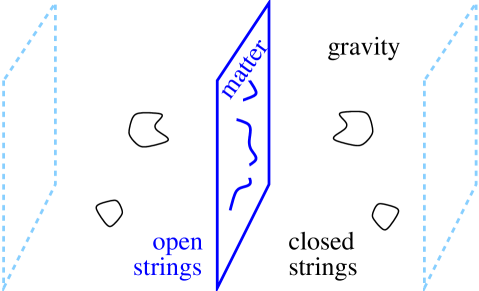
Figure 1: Matter fields are described by open strings confined to branes.

This lead several authors to consider the possibility that at least some of the extra dimensions could be far larger than had previously been imagined A ; AADD . They realised that while particle interactions are probed by high energy colliders on energies up to $1$ TeV, and hence scales down to $10^{-19}$ m, gravity is barely tested on scales below $1$ mm. If the extra dimensions were testable only via gravity then they might be relatively large. This offers a tantalising explanation for why gravity appears to be so weak when compared with the other interactions. The gravitational field of an object could leak out into the large but hidden dimensions and gravity in our four-dimensional world seems weaker.

To make this a little more precise, consider the gravitational field of a mass $M$ in a $D$-dimensional spacetime. If we use Gauss’s law to calculate the gravitational field strength $g$ at a distance $r$ then we find $g\propto G_{D}M/r^{D-2}$ for distances $r\ll R$, the radius of compactification of the hidden dimensions. But if $r\gg R$ then the gravitational field strength is given by

$$g=\frac{4\pi G_{D}M}{4\pi r^{2}R^{D-4}}\,.$$ (3)

The effective value of Newton’s constant in our apparently 4-dimensional world, $G_{4}$, can be identified as

$$G_{4}\equiv\frac{G_{D}}{R^{D-4}}\,.$$ (4)

Given we observe only the four-dimensional effective gravitational coupling, from which we infer a very large effective Planck scale $M_{4}=1/\sqrt{G_{4}}=10^{19}$ GeV, the true value of the Planck scale (the scale at which quantum gravity becomes important) could be much smaller in models with large extra dimensions.

For instance, Horava and Witten in 1996 HW96 proposed a supergravity model in 11-dimensions with a fundamental Planck scale close to the Grand Unified (GUT) scale of $10^{16}$ GeV where one of the extra dimensions had a size considerably larger than the conventional Planck scale of $10^{-35}$ m. But the GUT scale is still far beyond terrestrial experiments and established particle physics models. What if quantum gravity was within reach of experiments like the LHC at CERN? If one hidden dimension was as large as $1$ mm then the Planck scale could be as low as $10^{8}$ GeV. With two large extra dimensions, the Planck scale could be as low as $1$ TeV AADD .

3 Randall-Sundrum model

So far I have implicitly been discussing Minkowski branes in a higher dimensional Minkowski spacetime. This provides a good vacuum state for string theory but we need to go beyond flat spacetime to provide a cosmological model. Anti-de Sitter (AdS) spacetime, that is maximally symmetric space with a negative cosmological constant, $\Lambda^{2}=-6k^{2}$, can also provide a useful vacuum state for string theory. This may not appear to be very promising for a cosmological model as a negative cosmological constant leads to a cosmological collapse and big crunch in homogeneous and isotropic cosmologies. However it turns out to be a fascinating spacetime in which to consider brane-world cosmology.

Randall and Sundrum produced two papers RS1 ; RS2 in 1999 which have had a huge impact in string theory and cosmology. They considered gravity on constant tension branes embedded in five-dimensional anti-de Sitter spacetime.

Branes can be embedded at fixed $y$-coordinate in a Gaussian normal coordinate system where the AdS₅ metric is written as

$$ds^{2}=e^{-2k|y|}\eta_{\mu\nu}dx^{\mu}dx^{\nu}+dy^{2}\,.$$ (5)

The exponential “warp factor” means that the volume of the extra dimensional space becomes small at large $y$. In their first paper RS1 Randall and Sundrum showed that the large hierarchy between a fundamental TeV scale and the apparent Planck scale $10^{19}$ GeV could be “explained” by a large warp factor even if the size of the extra dimension (specifically the normal distance between branes) was relatively small. But in their second paper RS2 they showed that even if there was no second brane, and the extra dimension extended to infinity, gravity remained effectively localised on a single brane as the integrated volume remained finite as $y\to\infty$. This they proposed as an “alternative to compactification”.

Figure 2: Randall Sundrum 1, where the hierarchy between the Planck scale and the TeV scale is due to the distance between two branes in compact AdS spacetime.

Figure 3: Randall Sundrum 2, where there is only one brane embedded in non-compact 5D spacetime.

The two-brane model RS1 , called RS1, is not so different from earlier attempts to compactify the hidden dimensions, other than that it operates in a curved bulk spacetime. It is still the large volume of the hidden space that makes gravity weaker on the brane than other forces. There is still a discrete spectrum of Kaluza-Klein states corresponding to higher harmonics on the hidden space, although the spectrum of eigenvalues is different in a curved space. And the size of the extra dimension, the distance between the two branes remains a scalar degree of freedom, known as the radion. It still leads to an effective scalar-tensor gravity in four dimensions at low energies GT ; KS which may be in conflict with experimental tests unless the radion is stabilised.

On the other hand, the one-brane model RS2 , inevitably known as RS2, offers a radically different model of dimensional reduction. The radion field in the RS1 model, decouples from gravity on the remaining brane in the limit that the second brane tends to spatial infinity. (The Brans-Dicke parameter $\omega\to\infty$ GT ; KS .) And the discrete spectrum of KK modes is replaced with a continuum of bulk modes. However the lightest modes are only weakly coupled to matter on the brane and gravity remains effectively four-dimensional on length scales greater than the AdS curvature scale, $k^{-1}$. More fundamentally though the single brane in AdS is an open system now where the initial state of matter on the brane (or branes) is not enough to determine the future evolution of the system. Instead one needs to specify initial data on a Cauchy hypersurface in the bulk. For example one might specify the AdS incoming vacuum state Rubakov . And fields on the brane can radiate into the bulk and information can escape to future null infinity.

In either of the RS models there is a simple and novel interpretation of our cosmological expansion. In the curved anti-de Sitter bulk spacetime (5) any motion of the brane, represented by a time-dependent trajectory $y=y_{b}(t)$, induces an FRW metric on the brane with scale factor $a=e^{-k|y_{b}|}$ MSM ; BCG . Cosmological expansion on the brane corresponds to motion in a curved bulk spacetime.

4 Brane-world gravity

One way to understand the gravitational theory on a brane, such as the Randall-Sundrum branes in AdS, is to use the projected Einstein equations on the brane SMS ; Roy . Consider a codimension-one brane with unit normal vector $n^{A}$. The induced metric on the brane is then

$$g_{AB}=\,^{(5)}g_{AB}-n_{A}n_{B}\,,$$ (6)

and the extrinsic curvature of the brane is

$$K_{AB}=g^{AC}\,{}^{(5)}\nabla_{C}n_{B}\,.$$ (7)

The 4D Riemann tensor on the brane can be given in terms of the 5D Riemann tensor in the bulk and the brane’s extrinsic curvature as Roy

$$R_{ABCD}=^{(5)}R_{EFGH}\,g_{A}^{E}\,g_{B}^{F}\,g_{C}^{G}\,g_{D}^{H}+2K_{A[C}K_{D]B}\,.$$ (8)

The higher-dimensional Einstein equations (1) determine the bulk Einstein tensor in terms of the bulk energy-momentum tensor. In the case of a vacuum bulk with only a cosmological constant we have

$${}^{(5)}G_{AB}+\Lambda_{5}\,^{(5)}g_{AB}=0\,.$$ (9)

The Israel-Darmois junction conditions determine the jump in the extrinsic curvature tensor across the brane in terms of the energy-momentum tensor localised on the brane where $\kappa_{5}^{2}$ is the gravitational coupling constant in 5-dimensions. In the Randall-Sundrum model the brane is a boundary of the bulk spacetime. This is equivalent to imposing a $Z_{2}$-symmetry across the brane so that $K_{AB}=K_{AB}^{+}=-K_{AB}^{-}$ and hence

$$K_{AB}=-\frac{\kappa_{5}^{2}}{2}\left[T^{\rm brane}_{AB}-\frac{1}{3}T^{\rm brane}g_{AB}\right]\,.$$ (10)

This also occurs in the Horava-Witten model where the 10D boundary branes are fixed points of the orbifold $S_{1}/Z_{2}$. On the other hand the HW model also admits additional branes which can move within the bulk spacetime. In this case there is an additional freedom due to the averaged extrinsic curvature, $K_{AB}^{+}+K_{AB}^{-}$, which is not directly constrained by the energy-momentum tensor on the brane AndyMetal , but for simplicity I will assume $Z_{2}$-symmetry across the brane in the following.

Finally putting all this together we can give an expression for the Einstein tensor for the induced metric on the brane SMS

$$G_{AB}+\Lambda g_{AB}=\kappa_{4}^{2}T_{AB}+\kappa_{5}^{4}{\cal S}_{AB}-{\cal E}_{AB}\,,$$ (11)

where (i) ${\cal S}_{AB}$ and (ii) ${\cal E}_{AB}$ represent modifications to the standard Einstein equations (1) due to (i) terms quadratic in the brane energy-momentum tensor and (ii) the 5D Weyl tensor projected on the brane.

The 4D intrinsic curvature (8) includes terms quadratic in the extrinsic curvature of the brane, and hence, via (10), the energy-momentum on the brane. Indeed we only recover a term linear in $T_{AB}$ in Eq. (11) if the energy-momentum tensor on the brane contains a constant part due to a constant tension or vacuum energy density on the brane, $\sigma$, so that we split

$$T_{AB}^{\rm brane}=\sigma g_{AB}+T_{AB}\,.$$ (12)

The effective 4D gravitational coupling constant for the renormalised energy-momentum tensor, $T_{AB}$, in the brane-world Einstein equations (11) is then given by

$$\kappa_{4}^{2}=\frac{\kappa_{5}^{4}\sigma}{6}\,.$$ (13)

The effect of terms quadratic in the matter energy-momentum tensor is given by

$${\cal S}_{AB}=\frac{1}{12}TT_{AB}-\frac{1}{4}T_{AC}T_{B}^{C}+\frac{1}{24}g_{AB}\left(3T_{CD}T^{CD}-T^{2}\right)\,.$$ (14)

It is represents a high-energy correction to the brane-world Einstein equations and is typically unimportant when the matter density is much less than the brane tension, $\rho\ll\sigma$.

4.1 The brane-world cosmological constant problem

The effective cosmological constant on the brane in Eq. (11) is given by

$$\Lambda=\frac{\Lambda_{5}}{2}+\frac{\kappa_{5}^{4}\sigma^{2}}{12}\,.$$ (15)

In contrast to our usual 4D viewpoint that the vacuum energy density should simply vanish, or be very small, in the brane-world we require instead that there is a cancellation between the 4D and 5D contributions to the vacuum energy. An intriguing possibility in the brane-world is that 4D cosmological solutions might naturally seek out fixed points in an inhomogeneous 5D spacetime with small values of the cosmological constant – called self-tuning solutions selftune .

A novel twist on the cosmological constant problem is provided by the model of Dvali, Gabadadze and Porrati (DGP) DGP who pointed out that quantum loop corrections to any classical model would be expected to induce terms in the effective energy-momentum tensor on the brane proportional to the brane Einstein tensor: $\Delta T_{AB}^{\rm brane}=\alpha G_{AB}$. In a 4D model such corrections would simply renormalise the gravitational coupling $\kappa_{4}^{2}$. But substituted into (11) the brane-world Einstein equations become quadratic in the Einstein tensor. Thus in addition to the usual vacuum solution with $G_{AB}=0$ when $\Lambda=0$, there is a second (non-perturbative) solution with $G_{AB}\propto\alpha^{-2}g_{AB}$. The DGP model has sparked great interest as a novel explanation of the observed acceleration of our Universe Deffayet , in terms of modified gravity rather than “dark energy”, but there remain questions over whether the self-accelerating solutions admit unstable “ghost” modes KK .

4.2 Non-local brane gravity

Equation (11) leaves only the projected 5D Weyl tensor

$${\cal E}_{AB}=\,^{(5)}C_{ECFD}\,g_{A}^{E}\,g_{B}^{F}\,n^{C}\,n^{D}\,.$$ (16)

undetermined by the local energy-momentum on or near the brane. This is the tidal part of the 5D gravitational field so is only determined when one has a solution to the full 5D Einstein equations with appropriate boundary conditions.

To the brane-bound observer it may be interpreted as an effective “Weyl fluid” with energy density $\tilde{\rho}$ and 4-velocity $\tilde{u}_{A}$ so that Roy

$$-{\cal E}_{AB}=\kappa_{4}^{2}\left[\frac{\tilde{\rho}}{3}\left(g_{AB}+4\tilde{u}_{A}\tilde{u}_{B}\right)+\tilde{\Pi}_{AB}\right]\,.$$ (17)

Because of the symmetries of the bulk Weyl tensor, ${\cal E}_{AB}$ is trace-free and hence the Weyl fluid is trace-free and has be interpreted as “dark radiation” Kraus . This is consistent with the Maldacena’s AdS-CFT conjecture Maldacena which implies that the higher-dimensional gravitational field is equivalent to a conformal field theory on the boundary Gubser .

The 4D Bianchi identities, $\nabla^{A}G_{AB}=0$, imply from Eq. (11) that the Weyl fluid’s energy $\tilde{\rho}$ and momentum $\tilde{\rho}\tilde{u}_{A}$ obey local conservation equations on the brane, driven by the quadratic energy-momentum tensor

$$\nabla^{A}{\cal E}_{AB}=\kappa_{5}^{4}\nabla^{A}{\cal S}_{AB}\,.$$ (18)

The evolution of the Weyl anisotropic stress, $\tilde{\Pi}_{AB}$, however cannot in general be determined from initial conditions set solely on the brane. Thus while the projected equations, and the Weyl fluid description in particular, may be useful for interpreting 5D gravity as seen on the brane, it may be of limited use in deriving solutions. This intrinsic non-locality of 4D gravity in the brane-world is the reason why so many outstanding problems remain, including the nature of black hole solutions on the brane or anisotropic cosmologies, and require higher-dimensional solutions.

5 FRW cosmology on a brane

One, important, case in which the projected field equations are sufficient is the behaviour of 4D homogeneous and isotropic (FRW) cosmologies. In this case the maximal symmetry of 3D space requires that the Weyl anisotropic stress vanishes and the general form of the modified Friedmann equation (2) on the brane is

$$3\left(H^{2}+\frac{K}{a^{2}}\right)=\Lambda+\kappa_{4}^{2}\rho\left(1+\frac{\rho}{2\sigma}\right)+\frac{m}{a^{4}}\,,$$ (19)

where $m$ is an integration constant on the brane set by the initial density of the Weyl fluid or dark radiation on the brane.

In fact a generalisation of Birkhoff theorem implies that the general 5D vacuum spacetime admitting an FRW brane cosmology is Schwarzschild-Anti-de Sitter (SAdS) MSM ; BCG . The integration constant $m$ in (19) represents the mass of the black hole in the SAdS spacetime (though in a compact RS1 model the singularity may lie outside the physical region of the spacetime between the branes).

The cosmological expansion described by the modified Friedmann equation (19) can be interpreted as motion of the brane in a static, but curved bulk. The static bulk metric can be written as

$$ds^{2}=-f(R)dT^{2}+\frac{dR^{2}}{f(R)}+R^{2}d\Omega_{K}^{2}\,,$$ (20)

where $d\Omega_{K}^{2}$ is the line element on a maximally symmetric 3-space, curvature $K$, and

$$f(R)=K+\left(\frac{R}{\ell}\right)^{2}-\frac{m}{R^{2}}\,.$$ (21)

On the other hand if we choose a Gaussian normal coordinate in which the brane is at a fixed location $y=y_{b}$ then the line element becomes

$$ds^{2}=-n^{2}(\tau,\chi)d\tau^{2}+d\chi^{2}+a^{2}(\tau,\chi)d\Omega_{K}^{2}\,,$$ (22)

where the explicit forms of $n$ and $a$ are given in Ref. BDEL . The two coordinate systems are related by a pseudo-Lorentz transformation at the brane LMW

$$\left(\begin{array}[]{c}nd\tau\\ d\chi\end{array}\right)=\Lambda(\theta)\left(\begin{array}[]{c}\sqrt{f}dT\\ dR/\sqrt{f}\end{array}\right)\,,$$ (23)

where

$$\Lambda(\theta)\equiv\left(\begin{array}[]{cc}\cosh\theta&\sinh\theta\\ \sinh\theta&\cosh\theta\end{array}\right)$$ (24)

and the Lorentz factor due to the motion of the brane in the bulk coordinates is

$$\cosh\theta=\sqrt{1+\frac{R^{2}H^{2}}{f}}\,,$$ (25)

and $H$ is the Hubble expansion rate (19).

This offers a novel perspective on 4D cosmology, not least the cosmological singularity problem. For instance, Garriga and Sasaki showed that an inflating brane and its SAdS bulk can be created “out of nothing” by a de Sitter-brane instanton GarrigaSasaki . Others have tried to describe the big bang singularity on the brane as a singular event within a regular higher-dimensional bulk, see for example Refs. ekpyrotic ; pyro ; cyclic ; bucher ; bbbbbb .

5.1 Colliding FRW branes

One scenario that has attracted much attention is the ekpyrotic model ekpyrotic ; pyro where the Big Bang on the brane-world is identified as a collision between branes. In the original version a hidden brane traverses the bulk and when it hits the boundary brane its kinetic energy is released, heating our observable universe and initiating the hot Big Bang.

It turns out to be possible to give a complete description in general relativity of the collision of maximally symmetric codimension-one branes (or shells) in vacuum collide , similar to that envisaged in the original ekpyrotic model. Consider the simplest case of two incoming FRW brane-worlds (a and b) coalescing at a 3D collision surface to give one outgoing brane (c) as shown in Figure 4. The intervening regions (I, II and III) are necessarily SAdS in vacua. Thus the coordinate system on each brane (20) and in each bulk region (22) are related by pseudo-Lorentz transformations of the form given in (24).

Figure 4: Collision between branes (a) and (b), separated by region I, resulting in single outgoing brane (c) between regions II and III.

There is a simple geometrical constraint that the product of all the Lorentz transformations (24), as one completes a circuit around the collision surface, is unity Neronov ; collide

$$\Pi_{i}\Lambda(\theta_{i})=1\,.$$ (26)

The junction conditions (10) enable one to relate the corresponding jump in the extrinsic curvature across each brane to the energy density on the brane, and hence one obtains a general relativistic version of the local conservation of energy-momentum at the collision collide

$$\rho_{c}\cosh\theta_{c}=\rho_{a}\cosh\theta_{a}+\rho_{b}\cosh\theta_{b}\,.$$ (27)

It is remarkable that a geometrical identity (26) when combined with the general relativistic junction conditions (10) reduces to a formula (27) that is of exactly the same form as energy conservation in special relativity.

There is no curvature singularity at the brane collision and yet the collision does represent an abrupt change in the energy density and expansion rate on the brane.

In the original ekpyrotic scenario ekpyrotic the collision occurs between a moving bulk brane and a $Z_{2}$-symmetric boundary brane. The $Z_{2}$-symmetry at the boundary makes this equivalent to two symmetric bulk branes hitting the boundary at the same collision point. In principle one should also be able to calculate the spectrum of primordial perturbations inherited after the collision and thus test the model, see for instance Refs.ekpyrotic ; lyth . However, in the subsequent cyclic scenario cyclic the collision takes place between two $Z_{2}$-symmetric boundary branes, which is equivalent to an infinite number of branes colliding at the same hypersurface with an infinite energy density. Equivalently the fifth dimension disappears at the collision. This means that the collision really is singular even from the five-dimensional viewpoint and one cannot calculate the properties of any brane-world that emerges from the collision in any conventional (e.g., general relativistic) theory. Instead one has to construct a non-singular “completion” of the theory in order to eliminate the diverges, see, for example Ref.tolley .

5.2 Brane inflation

Branes have had a big impact in recent years upon attempts to construct models of inflation in the early universe within string theory. A long-standing problem has been the large number of light scalar fields, or moduli in the low-energy effective actions obtained from string theory. These would not only violate experimental tests of gravity today, as mentioned earlier, but also dilute the vacuum energy density required to drive inflation in the very early universe. But in recent years the inclusion of non-trivial anti-symmetric form fields on the hidden dimensions, so-called flux compactifications GKP , offer the possibility of stabilising all the moduli associated with the shape of the extra dimensions. The existence of branes plays a crucial role in providing a positive vacuum energy density in the low-energy effective theory.

Some of the resulting higher-dimensional geometries bear a close resemblance to the simple Randall-Sundrum brane-worlds. Near the branes the ten-dimensional spacetime may be distorted into a “throat” that is approximately described by AdS${}_{5}\times$S₅. This provides the setting, in the KKLT scenario KKLT , for brane-inflation DvaliTye in which the motion of the test branes in this warped geometry plays the role of an inflaton field. The collision of the branes signals the end of inflation and can also lead to a symmetry breaking phase transition on the brane.

These brane inflation models are constructed from low-energy effective potentials in a four-dimensional effective action. The dynamics during inflation is similar to models of hybrid inflation in four dimensional Einstein gravity originally derived from supergravity models in the 1990’s hybrid . In particular the moving branes are test branes moving in a fixed background geometry, quite different from the self-gravitating branes in higher-dimensional gravity that I discussed earlier. It remains to be seen if it is possible to describe popular models of brane inflation in the covariant approach of Shiromizu, Maeda and Sasaki, and whether the gravitational backreaction of the branes can be taken into account, and whether it plays an important role. For tentative steps in this direction see KKKK ; Mukohyama ; KSW .

5.3 Slow-roll inflaton on a brane

A simple way to study the effect of higher-dimensional gravity on inflation models is to consider inflation driven by the potential energy, $V$, of a four-dimensional inflaton field, $\phi$, confined to a brane, embedded in a vacuum bulk MWBH .

At low energies, $\rho\ll\sigma$, we have seen that we can recover the conventional Friedmann equation for the cosmological expansion. On the other hand, at high energies the additional quadratic term in the modified Friedmann equation (19) leads to additional Hubble damping and actually assists slow-roll inflation. The conventional slow-roll parameters, which must be much smaller than unity for slow-roll inflation, become

$$\epsilon=\frac{1}{16\pi G_{N}}\left(\frac{V^{\prime}}{V}\right)^{2} \to \left(\frac{4\sigma}{V}\right)\frac{1}{16\pi G_{N}}\left(\frac{V^{\prime}}{V}\right)^{2}\,,$$ (28)

$$\eta=\frac{1}{8\pi G_{N}}\left(\frac{V^{\prime\prime}}{V}\right) \to \left(\frac{2\sigma}{V}\right)\frac{1}{8\pi G_{N}}\left(\frac{V^{\prime\prime}}{V}\right)\,,$$ (29)

where a prime denotes derivatives with respect to $\phi$. The slow-roll parameters are automatically suppressed at high energies MWBH , even for potentials that might otherwise be considered too steep to drive inflation steep .

To lowest order in the slow-roll approximation it is remarkably easy to calculate the primordial perturbation spectra expected to be generated by an inflaton on the brane. Quantum fluctuations of a light scalar field ($|\eta|\ll 1$) in four-dimensional de Sitter spacetime ($\epsilon\ll 1$) give the standard result for the power spectrum of inflaton fluctuations on the Hubble scale ($k=aH$)

$${\cal P}_{\delta\phi}\simeq\left(\frac{H}{2\pi}\right)^{2}\,.$$ (30)

This determines the dimensionless curvature perturbation on uniform-density hypersurfaces MWBH

$${\cal P}_{\zeta}\simeq\left(\frac{H^{2}}{2\pi\dot{\phi}}\right)^{2}\,.$$ (31)

This is conserved on large (super-Hubble) scales for adiabatic density perturbations, even in brane-world gravity LMSW , simply as a consequence of local energy conservation WMLL ; conserved . Thus the standard expression (31) gives the initial (primordial) density perturbations from slow-roll inflation driven by an inflaton on the brane. Of course the actual values for $H$ and $\dot{\phi}$ in terms of the scalar field potential will differ due to the modified Friedmann equation at high energies.

To determine the amplitude of gravitational waves we do need to consider the five-dimensional metric perturbations. For a de Sitter brane in AdS₅ the wave equation is separable. We find a discrete zero-mode (as in the original Randall-Sundrum model) and a continuum of massive modes in the four-dimensional effective theory with $m^{2}>9H^{2}/4$ GarrigaSasaki . These massive modes are not excited by the de Sitter expansion – they remain in their vacuum state – and hence we need only consider the spectrum of tensor perturbations on super-Hubble scales from zero-mode vacuum fluctuations LMW ; Rubakov

$${\cal P}_{T}=F(V/\sigma)64\pi G\left(\frac{H}{2\pi}\right)^{2}\,,$$ (32)

where $F(V/\sigma)$ represents the enhancement with respect to the standard four-dimensional result. At low-energies we have $F\to 1$ but at high energies we find $F\simeq 3V^{2}/4\sigma^{2}\gg 1$. Nonetheless one can verify that the standard consistency relation between observables Lidsey

$$\frac{{\cal P}_{T}}{{\cal P}_{\zeta}}\simeq-2n_{T}\,,$$ (33)

still holds, where $n_{T}\equiv d\ln{\cal P}_{T}/d\ln k$ is the spectral tilt of the tensor power spectrum. It is quite unexpected that the non-trivial 5D modifications to the expected power spectra from slow-roll inflation leave the four-dimensional consistency relation unaltered Lidsey ; Mariam .

5.4 Quantum fluctuations on the brane

The above calculation would be expected hold to lowest order in the slow-roll approximation where one neglects the coupling between scalar field perturbations and the metric perturbations. On the other hand there is a small but finite coupling between inflaton field fluctuations and the metric even in slow-roll inflation. In 4D general relativity Mukhanov M88 and Sasaki S86 showed how to consistently couple the linear field perturbations to the metric and hence one can derive small corrections to the scalar field fluctuations (30) during inflation.

One might expect something similar for an inflaton on the brane, but there are important differences. Although deviations from 4D gravity are small at low energies (indeed we have argued that for long-wavelength perturbations the curvature perturbation $\zeta$ is conserved as in general relativity), at high energies the brane perturbations are strongly coupled to bulk gravity. A perturbative calculation, introducing the coupling at first-order in the slow-roll parameters, shows that there may be a damping effect on the small scale (sub-horizon) modes on a single brane at high energies Mizuno . This is not so surprising as the single brane in AdS bulk is an open system and high frequency modes on the brane are coupled to bulk gravitons that can escape to future null infinity. This highlights the need to treat the coupled brane-bulk system in a consistent way in order to define the initial vacuum state on an inflating brane. This remains another unsolved problem in brane cosmology.

Remarkably little work seems to have been done to investigate the quantum field theory of a boundary (brane) field coupled to a higher-dimensional (bulk) field. Recently George George considered a linear oscillator in flat spacetime linearly coupled to another linear oscillator on its boundary. Above a critical coupling one finds an instability corresponding to a discrete tachyonic bound state. This has been extended Mennim , to the case of a Minkowski boundary in an AdS bulk (i.e., a Randall-Sundrum geometry). Again we found a critical coupling above which there exists an unstable bound state. But even for weak coupling one finds a small imaginary part in the frequency of resonant modes (quasi-normal modes Sanjeev ) of the coupled brane-bulk oscillators, which indicates the slow decay of oscillations on the brane. This is an example of an effect which would not be seen in a dimensionally-reduced low-energy effective theory which included only the zero-mode of the bulk field.

6 Conclusions

In summary, the brane-world has offered a novel perspective on many of the unsolved problems in cosmology including the number of spatial dimensions, the initial singularity and the cosmological constant problem.

There remain many unsolved problems even in the simplest case of a co-dimension one brane. There is no known solution for an isolated black hole on the brane. Indeed it has been conjectured that there is no static black hole solution on the brane Emparan . Only a few special cases are known for anisotropic brane cosmologies Fabbri . Even linear perturbations about FRW branes are restricted to special cases or numerical solutions as the wave equation in the bulk is not in general separable in a Gaussian normal coordinate system.

Some of these problems are techinical difficulties simply due to the extra complication of an inhomogeneous extra dimension, but some problems are also more fundamental. If we are seeking to describe a single brane in an infinite extra dimension that the brane alone does not form a closed system and we must specify initial data in the bulk to determine the subsequent evolution.

A century after Einstein introduced physicists to four-dimensional spacetime, brane-worlds offer a big new higher-dimensional playground for relativists to explore. Cosmological models provide one area to study. If we can understand more about gravity in higher-dimensions then cosmology should also provide an opportunity to test these exotic ideas against observational data.

References

- (1) R. Maartens, Living Rev. Rel. 7, 7 (2004) [arXiv:gr-qc/0312059].
- (2) M. Gasperini and G. Veneziano, Phys. Rept. 373, 1 (2003) [arXiv:hep-th/0207130].
- (3) M. B. Green, J. H. Schwarz and E. Witten, Superstring Theory. Vol. 1: Introduction, Cambridge University Press, Cambridge, 1987.
- (4) T. Kaluza, Sitzungsber. Preuss. Akad. Wiss. Berlin (Math. Phys. ) 1921, 966 (1921).
- (5) J. Polchinski, String theory. Vol. 2: Superstring theory and beyond, Cambridge University Press, Cambridge, 1998.
- (6) I. Antoniadis, Phys. Lett. B 246, 377 (1990);
- (7) N. Arkani-Hamed, S. Dimopoulos and G. R. Dvali, Phys. Lett. B 429, 263 (1998) [arXiv:hep-ph/9803315]; I. Antoniadis, N. Arkani-Hamed, S. Dimopoulos and G. R. Dvali, Phys. Lett. B 436, 257 (1998) [arXiv:hep-ph/9804398].
- (8) P. Horava and E. Witten, Nucl. Phys. B 460, 506 (1996) [arXiv:hep-th/9510209].
- (9) L. Randall and R. Sundrum, Phys. Rev. Lett. 83, 3370 (1999) [arXiv:hep-ph/9905221].
- (10) L. Randall and R. Sundrum, Phys. Rev. Lett. 83, 4690 (1999) [arXiv:hep-th/9906064].
- (11) J. Garriga and T. Tanaka, Phys. Rev. Lett. 84, 2778 (2000) [arXiv:hep-th/9911055].
- (12) S. Kanno and J. Soda, Phys. Rev. D 66, 043526 (2002) [arXiv:hep-th/0205188].
- (13) D. S. Gorbunov, V. A. Rubakov and S. M. Sibiryakov, JHEP 0110, 015 (2001) [arXiv:hep-th/0108017].
- (14) S. Mukohyama, T. Shiromizu and K. i. Maeda, Phys. Rev. D 62, 024028 (2000) [Erratum-ibid. D 63, 029901 (2001)] [arXiv:hep-th/9912287].
- (15) P. Bowcock, C. Charmousis and R. Gregory, Class. Quant. Grav. 17, 4745 (2000) [arXiv:hep-th/0007177].
- (16) T. Shiromizu, K. i. Maeda and M. Sasaki, Phys. Rev. D 62, 024012 (2000) [arXiv:gr-qc/9910076].
- (17) R. A. Battye, B. Carter, A. Mennim and J. P. Uzan, Phys. Rev. D 64, 124007 (2001) [arXiv:hep-th/0105091].
- (18) N. Arkani-Hamed, S. Dimopoulos, N. Kaloper and R. Sundrum, Phys. Lett. B 480, 193 (2000) [arXiv:hep-th/0001197]; S. Kachru, M. B. Schulz and E. Silverstein, Phys. Rev. D 62, 045021 (2000) [arXiv:hep-th/0001206].
- (19) G. R. Dvali, G. Gabadadze and M. Porrati, Phys. Lett. B 485, 208 (2000) [arXiv:hep-th/0005016].
- (20) C. Deffayet, G. R. Dvali and G. Gabadadze, Phys. Rev. D 65, 044023 (2002) [arXiv:astro-ph/0105068].
- (21) D. Gorbunov, K. Koyama and S. Sibiryakov, arXiv:hep-th/0512097.
- (22) P. Kraus, JHEP 9912, 011 (1999) [arXiv:hep-th/9910149].
- (23) J. M. Maldacena, Adv. Theor. Math. Phys. 2, 231 (1998) [Int. J. Theor. Phys. 38, 1113 (1999)] [arXiv:hep-th/9711200].
- (24) S. S. Gubser, Phys. Rev. D 63, 084017 (2001) [arXiv:hep-th/9912001].
- (25) P. Binetruy, C. Deffayet, U. Ellwanger and D. Langlois, Phys. Lett. B 477, 285 (2000) [arXiv:hep-th/9910219].
- (26) D. Langlois, K. i. Maeda and D. Wands, Phys. Rev. Lett. 88, 181301 (2002) [arXiv:gr-qc/0111013].
- (27) D. Langlois, R. Maartens and D. Wands, Phys. Lett. B 489, 259 (2000) [arXiv:hep-th/0006007].
- (28) J. Garriga and M. Sasaki, Phys. Rev. D 62, 043523 (2000) [arXiv:hep-th/9912118].
- (29) J. Khoury, B. A. Ovrut, P. J. Steinhardt and N. Turok, Phys. Rev. D 64, 123522 (2001) [arXiv:hep-th/0103239].
- (30) R. Kallosh, L. Kofman and A. D. Linde, Phys. Rev. D 64, 123523 (2001) [arXiv:hep-th/0104073].
- (31) P. J. Steinhardt and N. Turok, Phys. Rev. D 65, 126003 (2002) [arXiv:hep-th/0111098].
- (32) J. J. Blanco-Pillado and M. Bucher, Phys. Rev. D 65, 083517 (2002) [arXiv:hep-th/0111089]; J. J. Blanco-Pillado, M. Bucher, S. Ghassemi and F. Glanois, Phys. Rev. D 69, 103515 (2004) [arXiv:hep-th/0306151].
- (33) U. Gen, A. Ishibashi and T. Tanaka, Phys. Rev. D 66, 023519 (2002) [arXiv:hep-th/0110286].
- (34) A. Neronov, JHEP 0111, 007 (2001) [arXiv:hep-th/0109090].
- (35) D. H. Lyth, Phys. Lett. B 524, 1 (2002) [arXiv:hep-ph/0106153]; J. Khoury, B. A. Ovrut, P. J. Steinhardt and N. Turok, Phys. Rev. D 66, 046005 (2002) [arXiv:hep-th/0109050].
- (36) A. J. Tolley and N. Turok, Phys. Rev. D 66, 106005 (2002) [arXiv:hep-th/0204091]; A. J. Tolley, N. Turok and P. J. Steinhardt, Phys. Rev. D 69, 106005 (2004) [arXiv:hep-th/0306109].
- (37) S. B. Giddings, S. Kachru and J. Polchinski, Phys. Rev. D 66, 106006 (2002) [arXiv:hep-th/0105097].
- (38) S. Kachru, R. Kallosh, A. Linde and S. P. Trivedi, Phys. Rev. D 68, 046005 (2003) [arXiv:hep-th/0301240].
- (39) G. R. Dvali and S. H. H. Tye, Phys. Lett. B 450, 72 (1999) [arXiv:hep-ph/9812483].
- (40) A. D. Linde, Phys. Rev. D 49, 748 (1994) [arXiv:astro-ph/9307002]; E. J. Copeland, A. R. Liddle, D. H. Lyth, E. D. Stewart and D. Wands, Phys. Rev. D 49, 6410 (1994) [arXiv:astro-ph/9401011].
- (41) Class. Quant. Grav. 22, 3431 (2005) [arXiv:hep-th/0505256].
- (42) S. Mukohyama, Y. Sendouda, H. Yoshiguchi and S. Kinoshita, JCAP 0507, 013 (2005) [arXiv:hep-th/0506050].
- (43) S. Kanno, J. Soda and D. Wands, JCAP 0508, 002 (2005) [arXiv:hep-th/0506167].
- (44) R. Maartens, D. Wands, B. A. Bassett and I. Heard, Phys. Rev. D 62, 041301 (2000) [arXiv:hep-ph/9912464].
- (45) E. J. Copeland, A. R. Liddle and J. E. Lidsey, Phys. Rev. D 64, 023509 (2001) [arXiv:astro-ph/0006421].
- (46) D. Langlois, R. Maartens, M. Sasaki and D. Wands, Phys. Rev. D 63, 084009 (2001) [arXiv:hep-th/0012044].
- (47) D. Wands, K. A. Malik, D. H. Lyth and A. R. Liddle, Phys. Rev. D 62, 043527 (2000) [arXiv:astro-ph/0003278].
- (48) D. H. Lyth and D. Wands, Phys. Rev. D 68, 103515 (2003) [arXiv:astro-ph/0306498].
- (49) G. Huey and J. E. Lidsey, Phys. Lett. B 514, 217 (2001) [arXiv:astro-ph/0104006].
- (50) M. Bouhmadi-Lopez, R. Maartens and D. Wands, Phys. Rev. D 70, 123519 (2004) [arXiv:hep-th/0407162].
- (51) V. F. Mukhanov, Sov. Phys. JETP 67, 1297 (1988) [Zh. Eksp. Teor. Fiz. 94N7, 1 (1988)].
- (52) M. Sasaki, Prog. Theor. Phys. 76, 1036 (1986).
- (53) K. Koyama, S. Mizuno and D. Wands, JCAP 0508, 009 (2005) [arXiv:hep-th/0506102].
- (54) A. George, J. Phys. A 38, 7399 (2005) [arXiv:hep-th/0412067].
- (55) K. Koyama, A. Mennim and D. Wands, Phys. Rev. D 72, 064001 (2005) [arXiv:hep-th/0504201].
- (56) S. S. Seahra, Phys. Rev. D 72, 066002 (2005) [arXiv:hep-th/0501175].
- (57) R. Emparan, J. Garcia-Bellido and N. Kaloper, JHEP 0301, 079 (2003) [arXiv:hep-th/0212132].
- (58) A. Fabbri, D. Langlois, D. A. Steer and R. Zegers, JHEP 0409, 025 (2004) [arXiv:hep-th/0407262].