Considerations on the excitation of black hole quasinormal modes

Abstract

We provide some considerations on the excitation of black hole quasinormal modes (QNMs) in different physical scenarios. Considering a simple model in which a stream of particles accretes onto a black hole, we show that resonant QNM excitation by hyperaccretion requires a significant amount of fine-tuning, and is quite unlikely to occur in nature. Then we summarize and discuss present estimates of black hole QNM excitation from gravitational collapse, distorted black holes and head-on black hole collisions. We emphasize the areas that, in our opinion, are in urgent need of further investigation from the point of view of gravitational wave source modeling.

A leading candidate source of detectable waves for Earth-based interferometers such as LIGO, Virgo, GEO600 and TAMA, as well as for the space-based interferometer LISA, is the inspiral and merger of binary black holes. The waveform should comprise three parts, usually referred to as inspiral, merger and ringdown. The inspiral waveform, originating from that part of the decaying orbit leading up to the innermost stable orbit, can be analyzed using post-Newtonian theory. Extensive studies of the detectability of this phase of the signal have been carried out, both for Earth-based BCV and for space-based interferometers BBW . The nature of the merger waveform is largely unknown at present, and is the subject of work in numerical relativity.

The ringdown waveform originates from the distorted final black hole, and consists of a superposition of quasi-normal modes (QNMs). Each mode has an oscillation frequency and a damping time that are uniquely determined by the mass $M$ and specific angular momentum $j\equiv J/M^{2}$ of the black hole kokkotas . The amplitudes and phases of the various modes are determined by the specific process that formed the final hole.

The uniqueness of the modes’ frequencies and damping times is directly related to the “no hair” theorem of general relativistic black holes. Therefore a reliable detection and accurate identification of QNMs could provide the “smoking gun” for black holes and an important test of general relativity in the strong-field regime dreyer .

The detectability of ringdown waves, and the accuracy with which we can measure their frequencies and damping times to test the no-hair theorem, depend mainly on the energy carried by each mode BCW . In turn, the energy distribution depends on the details of the merger process. Given our poor understanding of the merger phase, we have at best sketchy information concerning the energy distribution between different modes.

In the first part of this paper we show by a simple toy model that QNM excitation by infalling matter requires a significant amount of fine-tuning, and is quite unlikely in astrophysically realistic scenarios. In the second part we briefly review present estimates of QNM excitation in various physical situations, including gravitational collapse, simulations of single distorted black holes and head-on collisions of two black holes. This second part is an extended version of Sec. VB in BCW . Most of our considerations can be applied to the solar-mass black holes detectable by Earth-based interferometers, but the main motivation for this short review comes from our study of the massive black holes detectable by LISA BCW . Throughout this paper we use geometrical units ($G=c=1$).

1 Excitation by infalling matter

Various authors fhh ; AG suggested that quasinormal ringing could be resonantly excited by clumps of matter falling into the black hole at some appropriate rate. This rate should be such that the spatial separation of the clumps equals a multiple of the typical QNM wavelength. Here we show by a simple model that, in principle, the modes of a black hole can indeed be excited in this way. We also show that a simple addition of damped sinusoids provides a good fit of the resulting gravitational waveforms: in other words, we can interpret the resonant excitation of the modes in terms of interference between gravitational waves. For simplicity we consider clumps of mass $\mu$ much smaller than the black hole mass, $\mu\ll M$, so that we can apply a perturbative analysis.

Consider first one single clump falling from infinity. This process was first analyzed in a classical paper by Davis, Ruffini, Press and Price davis (hereafter DRPP). They found that the total radiated energy is $\simeq 0.0104\mu^{2}/M$, most of it ($0.0091\mu^{2}/M$) being emitted as quadrupolar ($\ell=2$) waves, and that the total energy spectrum is peaked at $\omega\sim 0.32/M$, very close to the fundamental $\ell=2$ QNM frequency $\omega\simeq 0.3737/M$.

We can now superpose the waveform and its Fourier transform for the one-particle case to represent two or more particles falling into a black hole and to study interference phenomena (we are assuming that the clumps are non-interacting, so that there is no extra contribution to the total energy-momentum tensor). A similar sum-over-point-particles approach has been used many times in the past pointptcles , but the particular process we consider here has not been studied before.

Let us first suppose that we drop two particles with a temporal separation of $T$ (which, bearing in mind that the retarded time is the measured quantity, also means a spatial separation of $T$ between the two bodies). If $\Psi_{1}(t,r)$ represents the waveform for the first body (normalized by $\mu$, where $\mu$ is the mass of the infalling body), then the total waveform will be

$$\Psi(t,r)=\mu\Psi_{1}(t,r)+\mu\Psi_{1}(t-T,r)\,.$$ (1)

Likewise the Fourier transform ${\tilde{\Psi}}(\omega,r)$ will be

$${\tilde{\Psi}}=\mu{\tilde{\Psi}_{1}}+\mu e^{i\omega T}{\tilde{\Psi}_{1}}\,.$$ (2)

For $N$ bodies dropped regularly, such that the temporal difference between the dropping of the first and of the last is $T$, we have

$$\Psi(t,r)=\sum_{j=0}^{N-1}\mu\Psi_{1}\left(t-\frac{iT\,}{N-1}j,r\right)\,,\quad{\tilde{\Psi}}(\omega,r)=\sum_{j=0}^{N-1}\mu e^{\frac{i\omega T}{N-1}j}{\tilde{\Psi}_{1}}\,.$$ (3)

The infall of a finite-sized body can also be studied with this formalism . Incidentally, one can prove that $|\mu\sum_{j=0}^{N-1}e^{\frac{i\omega T}{N-1}j}|^{2}\leq\mu^{2}N^{2}$, so the total energy $E_{\rm rad}\sim\omega^{2}|{\tilde{\Psi}}|^{2}$ radiated by a stream of plunging particles is always less than or equal to the energy radiated by a single point particle with total mass $\mu N$.

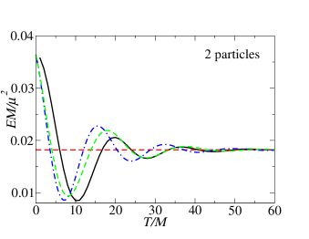
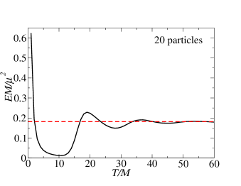
Figure 1: Characteristic interference pattern in the total energy radiated by two (left) and twenty (right) particles falling into a Schwarzschild black hole, as a function of the particles’ initial separation. As $T\to 0$ the particles behave as a single particle of mass $(N\mu)$, and the total energy scales like $(N\mu)^{2}$. The red, dashed horizontal line corresponds to the sum of the single-particle energies ($E\sim N\times 0.0091\mu^{2}/M$ for $N$ particles). In the two-particle case we also overplot the prediction of the two-mode ringdown waveform, Eq. (8). The blue, dot-dashed line corresponds to $\omega_{r}=0.3737/M$ (the fundamental QNM frequency with $\ell=2$). To obtain the green, dashed line we choose the “phenomenological” value $\omega_{r}=0.32/M$ (corresponding to the peak of the one-particle energy spectrum).

The total energy radiated in $\ell=2$ as a function of separation for two and twenty particles is shown in Fig. 1. Let us first consider the two-particle case (left panel). As we increase the distance between the two bodies the total energy decreases. At the first minimum ($T\sim 9.9M$) the total energy radiated is $\sim 0.0085\mu^{2}/M$. The next maximum is attained at $T\sim 19.8M$, the total radiated energy being $\simeq 0.0206\mu^{2}/M$. Since the one-particle spectrum is highly peaked at $\omega\sim 0.32/M$, it is tempting to explain this behavior as an interference phenomenon. The typical dominant wavelength of the fundamental QNM is $\lambda=2\pi/\omega\sim 19.6M$: this means that, for two particles, destructive interference should occur at $T\sim 9.8M$ and constructive interference at $T\sim 19.6M$, in good agreement with our numerical results. In the limit of large distances, interference becomes negligible and the total radiated energy tends to the sum of the individual particle energies ($\simeq 0.0182\mu^{2}/M$ for our two particles). This interpretation of the result is confirmed by an explicit calculation of the gravitational waveforms (Fig. 2).

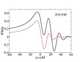
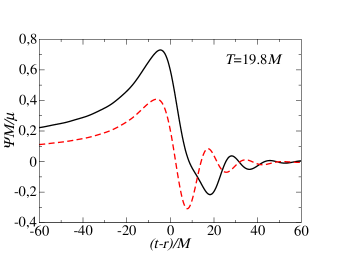
Figure 2: Two-particle waveforms (solid black lines) are compared with the single-particle waveforms (dashed red lines). In the left panel $T=9.9M$, and the ringdown is suppressed by destructive interference. In the right panel $T=19.8M$, and the ringdown is enhanced by constructive interference.

The situation for more than two particles is similar. Notice that in the two-particle case, for $T<6M$ there is always an enhancement on the total radiated energy (as compared to the sum of the single-particle energies). However, as we increase the number of particles, this enhancement interval decreases. So we should expect it will be hard to resonantly excite the black hole QNMs using a large number of particles.

Interpreting the results in terms of ringdown waveforms - The DRPP signal is dominated by quasinormal ringing, so it makes sense to try and interpret the preceding results in terms of ringdown waveforms. To start with, we assume our signal has the form

$$\psi=\Theta(t)Ae^{-\omega_{i}t}\sin{\omega_{r}t}\,,$$ (4)

where $\Theta(t)$ is the Heaviside function. For the fundamental mode of a Schwarzschild black hole $\omega_{r}\simeq 0.3737/M$ and $\omega_{i}\simeq 0.0890/M$. The amplitude $A$ can be obtained imposing that the total radiated energy in $\ell=2$ is equal to $0.0091\mu^{2}/M$. The total energy radiated in the $\ell$-th multipole is

$$E_{\rm rad}=\frac{1}{64\pi}\frac{(l+2)!}{(l-2)!}\int_{-\infty}^{-\infty}\left(\frac{d\psi}{dt}\right)^{2}dt\,,$$ (5)

which for the waveform (4) gives

$$E_{\rm rad}=\frac{A^{2}(l+2)!\omega_{r}^{2}}{256\pi(l-2)!\omega_{i}}\,.$$ (6)

Setting $\ell=2$ and equating this to $0.0091\mu^{2}/M$ gives $A\simeq 0.441\mu$, in qualitative agreement with the DRPP waveform. Let us now consider two particles by superposing two ringdown waveforms:

$$\psi=\Theta(t)Ae^{-\omega_{i}t}\sin{\omega_{r}t}+\Theta(t-T)Ae^{-\omega_{i}(t-T)}\sin{\omega_{r}(t-T)}\,.$$ (7)

The total energy radiated would be

$$E_{\rm rad}^{\rm 2ptcles}=\frac{A^{2}e^{-T\omega_{i}}\omega_{r}(l+2)!}{128\pi(l-2)!\omega_{i}}\left(e^{\omega_{i}T}\omega_{r}+\omega_{r}\cos{\omega_{r}T}-\omega_{i}\sin\omega_{r}T\right)\,.$$ (8)

A plot of this function is shown in the left panel of Fig. 1. It is in good qualitative agreement with the full numerical calculation. If we use a “phenomenological” QNM frequency $\omega_{r}=0.32/M$ (corresponding to the peak of the one-particle energy spectrum, and yielding an amplitude $A\simeq 0.515\mu$) instead of the “true” fundamental $\ell=2$ QNM frequency $\omega_{r}=0.3737/M$, the agreement between Eq. (8) and the numerical results becomes even better.

This agreement suggests the possibility to extend our study to Kerr black holes, by simply assuming that $\omega_{r}$ and $\omega_{i}$ are functions of the black hole’s angular momentum. Using (6) and (8) we get

$$\frac{E_{\rm rad}^{\rm 2ptcles}}{E_{\rm rad}}=2e^{-T\omega_{i}}\left(e^{\omega_{i}T}+\cos{\omega_{r}T}-\frac{\omega_{i}}{\omega_{r}}\sin\omega_{r}T\right)\sim 2(1+\cos\omega_{r}T)\,.$$ (9)

In the last step we considered rapidly rotating (near-extremal) black holes and modes with $\ell=m$, for which $\omega_{i}\rightarrow 0$ and $\omega_{r}\rightarrow m/(2M)$. Therefore, for corotating modes of rapidly rotating black holes the resonance is almost perfect if we choose $T=2\pi M/m$ (the ratio is then 4, the maximum allowed) while destructive interference results if $T=\pi M/m$.

In summary: constructive resonance, and consequently QNM excitation, is possible (in principle) when a stream of particles accretes onto a black hole. Unfortunately, the separation between each particle required for an enhancement in the total energy becomes very small as the number of particles increases. Unless some delicate fine tuning is at work AG , the separation between any two infalling particles or clumps should be driven by a random process, which means that on average there should be no resonance at all. This is confirmed by simulations of generic configurations of infalling matter, where quasinormal ringing is usually absent from the waveforms nagar .

2 Energy distribution in different scenarios

In this Section we present a brief review of results on QNM excitation in different physical scenarios, including gravitational collapse, evolutions of single distorted black holes and head-on black hole collisions. Far from being complete or comprehensive, our review aims to emphasize areas that require further investigation from the point of view of gravitational wave source modeling.

Gravitational collapse - There are just a few calculations of gravitational wave emission from rotating gravitational collapse to a black hole. Perturbative calculations were first carried out by Cunningham, Price and Moncrief cpm1 ; cpm2 ; cpm3 , and later improved upon by Seidel and collaborators seidel . These studies suggest that gravitational waves are mainly generated in the region where the Zerilli (or Regge-Wheeler) potential is large, and that the signal is always dominated by quasinormal ringing of the finally formed black hole. Simplified simulations based on a free-fall (Oppenheimer-Snyder) collapse model yield a rather pessimistic energy output, with a typical core-collapse radiating up to $E\simeq 10^{-7}M$ in gravitational wave energy, and most of the radiation being emitted in modes with $\ell=2$. Radiation in $\ell=3$ is typically two to three orders of magnitude smaller than the $\ell=2$ radiation (see eg. Fig. 9 in cpm1 ). Cunningham et al. also provide analytical expressions for the energy radiated in different multipoles as a function of the initial quadrupole deformation of the star and of the initial collapse radius cpm1 ; cpm2 .

For a long time the only nonperturbative, axisymmetric calculation of gravitational wave emission from collapse has been provided by the seminal work of Stark and Piran starkpiran . Surprisingly, the waveform resembles that emitted by a point particle falling into a black hole, but with a reduced amplitude (we will see below that a similar result emerges from head-on black hole collisions in full general relativity). As expected for axisymmetric configurations, the amplitude of the cross polarization mode is always $<0.2$ that of the even mode, and the emission in the plus mode is dominantly quadrupolar, with a $\sin^{2}\theta$ angular dependence (the cross polarization has a dependence of the form $\cos\theta\sin^{2}\theta$). The total energy emitted is quite low; it increases with rotation rate, ranging from $\sim 10^{-8}M$ for $j=0$ to $\sim 7\times 10^{-4}M$ as $j\to 1$. Rotational effects halt the collapse for some critical value of $j=j_{\rm crit}$ which is very close to unity, and depends on the amount of artificial pressure reduction used to trigger the collapse. Stark and Piran find that the energy emitted scales as $j^{4}$ for low $j$: $E/M\simeq{\rm min}\{1.4\times 10^{-3}j^{4},\epsilon_{\rm max}\}$ for $0<j<j_{\rm crit}$, where $\epsilon_{\rm max}\sim 10^{-4}$ again depends on the amount of artificial pressure reduction used to trigger the collapse. The $h_{+}$ waveform is very well fitted by a combination of the two lowest QNMs with $\ell=2$ and it is only weakly sensitive to $j$, reflecting the weak dependence of the slowly-damped Kerr QNM frequencies on $j$.

This two-dimensional calculation has recently been improved upon using a three-dimensional code baiotti , but still keeping a high degree of axisymmetry (so only modes with $m=0$ are excited). Ref. baiotti picks as the initial configuration the most rapidly rotating, dynamically unstable model described by a polytropic EOS with $\Gamma=2$ and $K=100$, having a dimensionless rotation rate $\simeq 0.54$, and triggers collapse reducing the pressure by less than about $2\%$. Gravitational waves are extracted by a gauge-invariant approach in which the spacetime is matched with nonspherical perturbations of a Schwarzschild black hole. The “plus” polarization is essentially a superposition of modes with $\ell=2$ and $\ell=4$, and the “cross” polarization is a superposition of modes with $\ell=3$ and $\ell=5$. Fig. 1 in baiotti shows that the amplitude of the $\ell=2$ mode is about an order of magnitude larger than the amplitude of the $\ell=4$ mode, and Fig. 3 shows that the cross polarization is roughly suppressed by one order of magnitude with respect to the plus polarization, with maximum amplitudes in a ratio $|(r/M)h_{\times}|_{\rm max}/|(r/M)h_{+}|_{\rm max}\simeq 0.06$ (here $r$ denotes the distance between source and detector). Odd-parity perturbations should be zero in spacetimes with axial and equatorial symmetries: they are nonzero because of the rotationally induced coupling with even-parity perturbations cpm1 ; cpm2 ; cpm3 ; seidel . The maximum amplitude from these three-dimensional simulations is $|(r/M)h_{+}|_{\rm max}\simeq 0.00225$, about one order of magnitude smaller than the amplitude found by Stark and Piran. Correspondingly, the total energy lost to gravitational waves is $E\simeq 1.45\times 10^{-6}(M/M_{\odot})$. This is about two orders of magnitude smaller than the estimate by Stark and Piran for the same value of the angular momentum, but larger than the energy losses found in recent calculations of rotating stellar core collapse to protoneutron stars muller .

Distorted black holes - Distorted black hole simulations shed some light on the (crucial) issue of the dependence of QNM excitation on the initial data: that is, on the “shape” and “size” of the black hole distortion.

Ref. krivan carries out a pioneering study of linearized gravitational perturbations of the Kerr spacetime. Given initial data with a certain angular dependence - that is, assigned values of $(l,~{}m)$ - their study finds that modes with positive and negative $m$ are always excited together. The simultaneous excitation of corotating and counterrotating modes depends on a certain reflection-symmetry property of the Kerr QNM spectrum BCW , and is confirmed by more recent time-evolutions of scalar perturbations of the Kerr spacetime dorband . In addition, these new simulations show that the relative excitation of corotating and counterrotating modes depends on the radial profile of the initial data, confirming expectations based on analytic investigations of the same problem GA . Unfortunately, detailed studies of the excitation of gravitational perturbations of Kerr black holes in the perturbative regime are still lacking.

Ref. abrahams92 provides one of the first attempts to extract gravitational waveforms from non-linear simulations of distorted black holes. They use a two-dimensional code to evolve initial data corresponding to a single, nonrotating black hole superimposed with time-symmetric gravitational waves (Brill waves), extract gravitational waves using gauge-invariant perturbation theory and show that, for low-amplitude Brill waves, non-perturbative and perturbative waveforms with $\ell=2$ and $\ell=4$ are in good agreement.

A more complete analysis is due to Anninos et al. bernstein2 . They use three different initial data sets, corresponding to very different physical situations: non-rotating black holes distorted by time-symmetric Brill waves, distorted rotating black holes, and the time-symmetric “two black hole” Misner data. In all three cases the system quickly settles down to a nearly spherical (or oblate, for rotating holes) configuration. They study the dynamics of the black hole horizon monitoring the ratio of polar and equatorial circumference $C_{r}=C_{p}/C_{e}$, and find that the horizon oscillates at the QNM frequencies of the final black hole. Oscillations with $\ell=2$ and $\ell=4$ are well fitted by a superposition of the fundamental QNM and the first overtone. In the “black hole plus (small) Brill wave” case, even when the initial data contain a significant component with $\ell=4$ (that is, when the index $n$ in the analytic expression of the Brill wave is equal to 4) the $\ell=4$ component of the horizon distortion is a factor $\sim 10^{-4}$ smaller than the $\ell=2$ component (Figs. 2 and 3 in bernstein2 ). For Misner initial data, corresponding to colliding black holes, $\ell=2$ waves are also strongly dominant. An important conclusion of Ref. bernstein2 is that the dynamics of the apparent horizon geometry can be used not only to find the fundamental QNM frequency of the hole, but also its mass and angular momentum.

Brandt and Seidel BS present an extensive study of distorted, rotating “Kerr-like” black holes with a wide range of rotation parameters (as high as $j\simeq 0.87$). Quasinormal ringing is observed both in the even and in the odd components of the emitted radiation. The angular momentum parameter $j$ is well approximated by the simple fit $j=\sqrt{1-(-1.55+2.55C_{r})^{2}}$ (the fit being generally accurate within $\sim 2.5\%$): this means that a measurement of the horizon geometry provides a value of the rotation parameter. For black holes with $j>\sqrt{3}/2$, a Kerr black hole cannot be embedded in flat space: an alternative method to obtain $j$ consists in measuring the angle at which the embedding ceases to exist.

A crucial result of Ref. BS is that the black hole dynamics depend critically on the properties of the initial data sets. For example, initial data corresponding to nonlinear, odd perturbations produce oscillations of the Gaussian curvature at frequencies given by linear combinations of QNMs with $\ell=3$ and $\ell=5$, because of beating phenomena. In Sec. IVB, they present a method to “dig out” frequencies with stronger damping from the slowly-damped modes in a Fourier transform, which can find useful applications in gravitational-wave data analysis. Sec. V of BS presents waveforms corresponding to different initial distortions of the hole. Odd-parity distortions of Schwarzschild black holes (run “o1” in their terminology) produce a waveform in which $99.9\%$ of the energy is radiated in $\ell=3$, $0.05\%$ of the radiation goes into $\ell=2$, $0.02\%$ into $\ell=4$ and $0.0001\%$ into $\ell=5$; but for different “shapes” of the distortion (run “o2”) , the energy radiated in $\ell=5$ can be as large as $21\%$. Similarly, runs corresponding to distorted Kerr black holes (“r0” to “r5”) contain different mixtures of the different multipoles depending on the shape of the initial distortion and on the rotation rate of the black hole. As a trend, large rotation seems to yield a large $\ell=3$ component: the maximum corresponds to run “r4”, for which the $\ell=2$ component carries $92.1\%$ of the energy and $\ell=3$ carries $\sim 7\%$ of the energy.

Three-dimensional, non-axisymmetric evolutions are urgently needed. A handful of non-axisymmetric simulations can be found in Ref. allen . They find that the total energy radiated in a given multipole, $E_{\ell m}$, ranges from $E_{20}\sim 3\times 10^{-4}M$ to $E_{42}\sim 3\times 10^{-7}M$. Only modes with $\ell=2$, $m=0,~{}2$ and $\ell=4$, $m=0,~{}2$ should occur at linear order in the amplitude, all other modes being quadratic in the amplitude (for one of these “nonlinear” modes they find a completely negligible energy, $E_{62}\sim 10^{-10}M$).

In fact, one of the most interesting features introduced by nonlinearities is mode-mode coupling. Ref. zlochower studies this coupling in detail for nonrotating (Schwarzschild) black holes. Large-amplitude incident waves effectively add mass to the black hole, producing a small but visible “redshift” in the QNM frequencies. The waveform is also slightly shifted by nonlinearities. This nonlinear dephasing might be an important issue when applying matched-filtering techniques. On the other hand, when the amplitude $A$ of incident waves exceeds a certain threshold, nonlinearities amplify the outgoing wave, which of course is good news for detection. Beyond the “nonlinearity threshold” the outgoing amplitude of the $\ell$-th multipole scales as $A^{\ell/2}$. The reason is that, for ordinary spherical harmonics, $\left(Y_{\ell m}\right)^{k}\sim Y_{(k\ell)m}+$terms with smaller $\ell$. Given a linear incident wave with $\ell=2$, an $\ell=2k$ mode arises from order $k$ (and higher) nonlinear terms; this mode’s amplitude scales as $A^{k}+{\cal O}(A^{k+1})$. So, the quadratic coupling of an $(\ell=2,~{}m=0)$ mode with itself produces an $(\ell=4,~{}m=0)$ mode of order $A^{2}+{\cal O}(A^{3})$ (and higher), in addition to an $(\ell=2,~{}m=0)$ mode of order $A+{\cal O}(A^{2})$ (notice that $\ell=0$ is ruled out for gravitational perturbations, being non-radiative). In addition, nonlinearities produce beating phenomena. In general, quadratic terms of an harmonic with frequency $\omega$ contain the frequencies $(0,~{}2\omega)$, cubic terms contain $(\omega,~{}3\omega)$, and so on. The selection rules for mode coupling in Kerr backgrounds should be more interesting: even in the linear regime, the Lense-Thirring effect couples axial and polar perturbations of a slowly rotating star according to Laporte’s rule laporte . Mode couplings in the Kerr background can be very important for gravitational wave data analysis, and deserve further study.

In conclusion, simulations suggest that (at least in situations with a certain degree of symmetry) high overtones are heavily suppressed. Investigating an extensive catalogue of initial data, Ref. BS shows that we just don’t know how energy is going to be partitioned between different modes in a realistic merger event, unless we can predict with accuracy the shape of the initial data. Nonetheless, for data-analysis purposes it should be reasonable to assume that modes with $\ell=2$, $m=0,~{}\pm 2$ have the largest amplitude (the components with $|m|=2$ probably being dominant). The contribution from $\ell=4$, $m=0,~{}\pm 2$ could be smaller by about two orders of magnitude in energy. Modes with $\ell=3$ may also be relevant, especially at large rotation rates. Nonlinearities could produce a cascade of energy into higher-order modes, but we need more simulations with realistic initial data to assess the relevance of this effect for QNM detection.

Head-on black hole collisions -

In four dimensions, the total energy radiated by a freely-falling particle released from rest at infinity in the Schwarzschild spacetime davis ; ferrari is in surprising agreement with numerical simulations of head-on black hole collisions. An extensive comparison of numerical results with perturbation theory can be found in Refs. smarr ; anninos1 ; anninos2 ; closelimit ; anninosl4 .

Fig. 14 and Sec. IV of Ref. anninos2 show that the perturbation-theory prediction for the radiated energy, $E=0.0104\mu^{2}/M$ davis , is in excellent agreement with numerical results when we replace the particle’s mass by the system’s reduced mass. In fact, perturbation theory slightly overestimates the energy output predicted by numerical simulations, which (according to state-of-the-art simulations) is $E\simeq 0.0013M$ sperhake . In the so-called “particle-membrane” picture, this disagreement is compensated for multiplying the perturbative prediction by three fudge factors anninos2 : i) a factor $F_{r_{0}}$, accounting for the fact that in numerical simulations the infall starts at finite distance $r_{0}$; ii) a factor $F_{h}$ coming in because the black hole (unlike the falling particle) has finite size, and tidal deformations heat up the horizon; iii) a factor $F_{\rm abs}$ to account for reabsorption of the emitted gravitational waves by each black hole. If the collision starts at infinite separation, $F_{r_{0}}=1$; $F_{h}$ has a weak dependence on $r_{0}$, and tends to $F_{h}\simeq 0.86$ as $r_{0}\to\infty$; $F_{\rm abs}\simeq 0.99$ is even less relevant.

If the total energy output from head-on black hole collisions is well understood, unfortunately the relative excitation of higher multipoles with respect to $\ell=2$ is not. Ref. anninosl4 compares numerical calculations with the close-limit approximation (valid when the black holes are close enough to be considered as perturbations of a single Schwarzschild black hole) and with the particle-membrane approach. Fig. 12 of Ref. anninosl4 compares the radiated energy according to the close-limit approximation with results from the numerical simulations. Extraction of the $\ell=4$ component from the simulations is very sensitive to numerical noise, especially when the black holes are very close and the $\ell=4$ component is more heavily suppressed.

Numerical simulations have been extended to include unequal-mass black holes brandt and boosted black holes boosted ; boosted2 . More recently, mesh refinement techniques were used to obtain more reliable estimates of the energy radiated in $\ell=2$ sperhake . Even for highly boosted black holes, the agreement between perturbation theory (in the close-limit approximation) and numerical simulations is very good. Numerical studies of boosted black holes show that, fixing the initial separation between the holes, the energy radiated saturates at $E\sim 0.01M$ for very large values of the initial momentum of the holes (see eg. Fig. 2 of boosted2 ). Ref. boosted combines Newtonian dynamics and numerical simulations of boosted black holes to suggest that the maximum energy emission could actually be much lower than this, $E<0.0016M$. In general, these studies suggest that the role of the weak-field phase of the evolution is only to determine the momentum of the black holes when they start to interact nonlinearly, emitting most of the radiation in the ringdown phase. This expectation is confirmed by the comparison of perturbation theory and Post-Newtonian calculations simone : the bremsstrahlung radiation emitted by a particle at separations larger than $4M$ (in Schwarzschild coordinates) contributes only $\sim 3\%$ of the total energy, most of the radiation coming from the final (ringdown) phase.

3 Conclusions

Most numerical simulations so far consider nearly-axisymmetric situations, so they don’t have much to say about the distribution of energy between modes with different values of $(l,m)$ in a realistic black hole merger. This is a crucial issue for data analysis from ringdown waveforms BCW . Recently there has been some remarkable progress in non-axisymmetric simulations of black hole mergers (see eg. herrmann and references therein), but a discussion of these developments is beyond the scope of this paper.

Some estimates of the energy radiated in the plunge phase by solar-mass binaries of rotating black holes are provided by the effective-one-body approach EOB . The error introduced by extrapolating to supermassive black holes should not be too large, since the energy balance of black hole binaries involves a single fundamental scale (their total mass $M$). It is useful to compare the effective-one-body estimate with earlier estimates of the energy radiated in the plunge plus ringdown phases, as provided by the Lazarus approach Lazarus . For aligned (anti-aligned) spins and specific angular momenta $j_{1}=j_{2}=0.17$ ($j_{1}=j_{2}=0.25$) the effective-one-body approach predicts an energy release $\sim(0.6-0.9)\%M$ [$\sim(1-3)\%M$]. The Lazarus approach finds $\sim(1.7-1.9)\%M$ [$\sim(1.9-2.1)\%M$], respectively. In principle, the difference of these two estimates should bracket the most reasonable range of ringdown efficiencies. However, the overall error on both estimates is still too large to draw any definite conclusion. Numerical relativity should be able to provide a reliable answer to this problem within a very short time.

References

- (1) A. Buonanno, Y. Chen and M. Vallisneri, Phys. Rev. D 67, 024016 (2003).
- (2) E. Berti, A. Buonanno and C. M. Will, Phys. Rev. D 71, 084025 (2005).
- (3) K. D. Kokkotas and B. G. Schmidt, Living Rev. Rel. 2, 2 (1999); H.-P. Nollert, Class. Quantum Grav. 16, R159 (1999).
- (4) O. Dreyer, B. Kelly, B. Krishnan, L. S. Finn, D. Garrison and R. Lopez-Aleman, Class. Quantum Grav. 21, 787 (2004).
- (5) E. Berti, V. Cardoso and C. M. Will, gr-qc/0512160.
- (6) C. L. Fryer, D. E. Holz and S. A. Hughes, Astrophys. J. 565, 430 (2002).
- (7) R. A. Araya-Góchez, MNRAS 355, 336 (2004).
- (8) M. Davis, R. Ruffini, W. H. Press and R. H. Price, Phys. Rev. Lett. 27, 1466 (1971).
- (9) M. P. Haugan, S. L. Shapiro and I. Wasserman , Astrophys. J. 257, 283 (1982); S. L. Shapiro and I. Wasserman, Astrophys. J. 260, 838 (1982); L. I. Petrich, S. L. Shapiro and I. Wasserman , Astrophys. J. Suppl. Ser. 58, 297 (1985); T. Nakamura and K. Oohara, Phys. Lett. 98A, 403, (1983); T. Nakamura, K. Oohara and Y. Kojima, Prog. Theor. Phys. Suppl. 90 (1987).
- (10) P. Papadopoulos and J. A. Font, Phys. Rev. D 63, 044016 (2001); A. Nagar, G. Diaz, J. A. Pons and J. A. Font, Phys. Rev. D 69, 124028 (2004); A. Nagar, J. A. Font, O. Zanotti and R. De Pietri, Phys. Rev. D 72, 024007 (2005).
- (11) C. T. Cunningham, R. Price and V. Moncrief, Astrophys. J. 224, 643 (1978).
- (12) C. T. Cunningham, R. Price and V. Moncrief, Astrophys. J. 230, 870 (1979).
- (13) C. T. Cunningham, R. Price and V. Moncrief, Astrophys. J. 236, 674 (1980).
- (14) E. Seidel and T. Moore, Phys. Rev. D 35, 2287 (1987); E. Seidel, E. S. Myra and T. Moore, Phys. Rev. D 38, 2349 (1988); E. Seidel, Phys. Rev. D 42, 1884 (1990); E. Seidel, Phys. Rev. D 44, 950 (1991).
- (15) R. F. Stark and T. Piran, Phys. Rev. Lett. 55, 891 (1985); in Proceedings of the Workshop Dynamical Spacetimes and Numerical Relativity, Philadelphia (Cambridge University Press, Cambridge, U.K., 1986), pp. 40-73.
- (16) L. Baiotti, I. Hawke, L. Rezzolla and E. Schnetter, Phys. Rev. Lett. 94, 131101 (2005).
- (17) E. Müller et al., Astrophys. J. 603, 221 (2004).
- (18) W. Krivan, P. Laguna, P. Papadopoulos and N. Andersson, Phys. Rev. D 56, 3395 (1997).
- (19) N. Dorband, P. Diener, E. Schnetter, M. Tiglio and E. Berti, in preparation.
- (20) K. Glampedakis and N. Andersson, Phys. Rev. D 64, 104021 (2001). K. Glampedakis and N. Andersson, Class. Quantum Grav. 20, 3441 (2003).
- (21) A. Abrahams, D. Bernstein, D. Hobill, E. Seidel and L. Smarr, Phys. Rev. D 45, 3544 (1992).
- (22) P. Anninos, D. Bernstein, S. R. Brandt, D. Hobill, E. Seidel and L. Smarr, Phys. Rev. D 50, 3801 (1994).
- (23) S. R. Brandt and E. Seidel, Phys. Rev. D 52, 870 (1995).
- (24) G. Allen, K. Camarda and E. Seidel, gr-qc/9806036.
- (25) Y. Zlochower, R. Gomez, S. Husa, L. Lehner and J. Winicour, Phys. Rev. D 68, 084014 (2003).
- (26) S. Chandrasekhar and V. Ferrari, Proc. R. Soc. Lond. A 433, 423 (1991).
- (27) V. Ferrari and R. Ruffini, Phys. Lett. B 98, 381 (1981).
- (28) L. L. Smarr, in Sources of Gravitational Radiation, edited by L. L. Smarr (Cambridge Univ. Press, Cambridge, 1979).
- (29) P. Anninos, D. Hobill, E. Seidel, L. Smarr and W. M. Suen, Phys. Rev. Lett. 71, 2851 (1993).
- (30) P. Anninos, D. Hobill, E. Seidel, L. Smarr and W. M. Suen, Phys. Rev. D 52, 2044 (1995).
- (31) R. J. Gleiser, C. O. Nicasio, R. H. Price, and J. Pullin, Phys. Rev. Lett. 77, 4483 (1996);
- (32) P. Anninos, R. H. Price, J. Pullin, E. Seidel and W. M. Suen, Phys. Rev. D 52, 4462 (1995).
- (33) U. Sperhake, B. Kelly, P. Laguna, K. L. Smith, E. Schnetter, Phys. Rev. D 71, 124042 (2005).
- (34) P. Anninos and S. Brandt, Phys. Rev. Lett. 81, 508 (1998).
- (35) A. M. Abrahams and G. B. Cook, Phys. Rev. D 50, R2364 (1994).
- (36) J. Baker, A. M. Abrahams, P. Anninos, S. Brandt, R. Price, J. Pullin and E. Seidel, Phys. Rev. D 55, 829 (1997).
- (37) L. E. Simone, E. Poisson and C. M. Will, Phys. Rev. D 52, 4481 (1995).
- (38) F. Herrmann, D. Shoemaker and P. Laguna, gr-qc/0601026.
- (39) A. Buonanno, Y. Chen and T. Damour, gr-qc/0508067.
- (40) J. Baker, M. Campanelli, C. O. Lousto and R. Takahashi, Phys. Rev. D 69, 027505 (2004).