The Local Effects of Cosmological Variations in Physical ’Constants’ and Scalar Fields
II. Quasi-Spherical Spacetimes

Abstract

We investigate the conditions under which cosmological variations in physical ‘constants’ and scalar fields are detectable on the surface of local gravitationally-bound systems, such as planets, in non-spherically symmetric background spacetimes. The method of matched asymptotic expansions is used to deal with the large range of length scales that appear in the problem. We derive a sufficient condition for the local time variation of the scalar fields driving variations in ’constants’ to track their large-scale cosmological variation and show that this is consistent with our earlier conjecture derived from the spherically symmetric problem. We perform our analysis with spacetime backgrounds that are of Szekeres-Szafron type. They are approximately Schwarzschild in some locality and free of gravitational waves everywhere. At large distances, we assume that the spacetime matches smoothly onto a Friedmann background universe. We conclude that, independent of the details of the scalar-field theory describing the varying ‘constant’, the condition for its cosmological variations to be measured locally is almost always satisfied in physically realistic situations. The very small differences expected to be observed between different scales are quantified. This strengthens the proof given in our previous paper that local experiments see global variations by dropping the requirement of exact spherical symmetry. It provides a rigorous justification for using terrestrial experiments and solar system observations to constraint or detect any cosmological time variations in the traditional ‘constants’ of Nature in the case where non-spherical inhomogeneities exist.

PACS Nos: 98.80.Es, 98.80.Bp, 98.80.Cq   

I
Introduction

Over the past few years there has been a resurgence of observational and theoretical interest in the possibility that some of the fundamental ‘constants’ of Nature might be varying over cosmological timescales webb . In respect of two such ‘constants’, the fine structure constant, $\alpha$, and Newton’s ‘constant’ of gravitation, $G$, the idea of such variations is not new, and was proposed by authors such as Milne milne , Dirac dirac , and Gamow gam as a solution to some perceived cosmological problems of the day btip . At first, theoretical attempts to model such variations in constants were rather crude and equations derived under the assumption that constants like $G$ and $\alpha$ are true constants were simply altered by writing-in an explicit time variation. This approach was first superseded in the case of varying $G$ by the creation of scalar-tensor theories of gravity jordan , culminating in the standard form of Brans and Dicke bd in which $G$ varies through a dynamical scalar field which conserves energy and momentum and contributes to the curvature of spacetime by a means of a set of generalised gravitational field equations. More recently, such self-consistent descriptions of the spacetime variation of other constants, like $\alpha$ bek ; bsm , the electroweak couplings ewk , and the electron-proton mass ratio, $\mu$, bm have been formulated although most observational constraints in the literature are imposed by simply making constants into variables in formulae derived under the assumption that are constant.

The resurgence of interest in possible time variations in $\alpha$ and $\mu$ has been brought about by significant progress in high-precision quasar spectroscopy. In addition to quasar spectra, we also have available a growing number of laboratory, geochemical, and astronomical observations with which to constrain any local changes in the values of   these constants reviews . Studies of the variation of other constants, such as $G$, the electron-proton mass ratio, $\mu=m_{e}/m_{pr}$, and other standard model couplings, are confronted with an array of other data sources. The central question which this series of papers addresses is how to these disparate observations, made over vastly differing scales, can be combined to give reliable constraints on the allowed global variations of $\alpha$ and the other constants. If $\alpha$ varies on cosmological scales that are gravitationally unbound and participate in the Hubble expansion of the universe, will we see any trace of this variation in a laboratory experiment on Earth? After all, we would not expect to find the expansion of the universe revealed by any local expansion of the Earth. In Paper I shawbarrow1 , we examined this question in detail for spherically symmetric inhomogeneous universes that model the situation of a planet or a galaxy in an expanding Friedmann-Robertson-Walker (FRW)-like universe. In this paper we relax the strong assumption of spherical symmetry and examine the situation of local observations in a universe that contains non-spherically symmetric inhomogeneity. Specifically, we use the inhomogeneous metrics found by Szekeres to describe a non-spherically symmetric universe containing a static star or planet. As in Paper I, we are interested in determining the difference (if any) between variations of a supposed ’constant’ or associated scalar field when observed locally, on the surface of the planet or star, and on cosmological scales.

When a ‘constant’, $\mathbb{C}$, is made dynamical we can allow it to vary by making it a function of a new scalar field, $\mathbb{C}\rightarrow\mathbb{C}(\phi)$, that depends on spacetime coordinates: $\phi=\phi(\vec{x},t)$. It has become general practice to combine take all observational bounds on the allowed variations of $\mathbb{C}(\phi)$. This practice assumes implicitly that any time variation of $\mathbb{C,}$ on or near the Earth, is comparable to any cosmological variation that it might experience, that is to high precision

$$\dot{\phi}(\vec{x},t)\approx\dot{\phi}_{c}(t),$$ (1)

for almost all locations $\vec{x}$, where $\phi_{c}$ is the cosmological value of $\phi$. This assumption is always made without proof, and there is certainly no a priori reason why it should be valid. Strictly, $\phi$ mediates a new or ‘fifth’ force of Nature. If the assumed behaviour is correct then this force is unique amongst the fundamental forces in that its value locally reflects its cosmological variation directly.

In this series of papers we are primarily interested in theories where the scalar field, or ‘dilaton’ as we shall refer to it, $\phi$, evolves according to the conservation equation

$$\square\phi=B_{,\phi}(\phi)\kappa T-V_{,\phi}(\phi),$$

where $T$ is the trace of the energy momentum tensor, $T=T_{\mu}^{\mu}$, (with the contribution from any cosmological constant neglected). We absorb any dilaton-to-cosmological constant coupling into the definition of $V(\phi)$. The dilaton-to-matter coupling $B(\phi)$ and the self-interaction potential, $V(\phi)$, are arbitrary functions of $\phi$ and units are defined by $\kappa=8\pi G$ and $c=\hslash=1$. This covers a wide range of theories which describe the spacetime variation of ‘constants’ of Nature; it includes Einstein-frame Brans-Dicke (BD) and all other, single-field, scalar-tensor theories of gravity bd ; bsm ; poly ; posp . In cosmologies that are composed of perfect fluids and a cosmological constant, it will also contain the Bekenstein-Sandvik-Barrow-Magueijo (BSBM) theory of varying $\alpha$, bsm , and other single-dilaton theories which describe the variation of standard model couplings, posp . We considered some other possible generalisations in shawbarrow1 . It should be noted that our analysis and results apply equally well to any theory which involves weakly-coupled, ‘light’, scalar fields, and not just those that describe variations of the standard constants of physics.

In first paper of this series, shawbarrow1 , we determined the conditions under which condition 1 would hold near the surface of a virialised over-density of matter, such as a galaxy or star, or a planet, such as the Earth, under the assumption of spherical symmetry. We chose to refer to this object as our ‘star’. In Paper I, matched asymptotic expansions were employed to analyse the most general, spherically-symmetric, dust plus cosmological constant embeddings of the ‘star’ into an expanding, asymptotically homogeneous and isotropic spherically symmetric universe. We proved that, independent of the details of the scalar-field theory describing the varying ‘constant’, that 1 is almost always satisfied under physically realistic conditions. The latter condition was quantified in terms of an integral over sources that can be evaluated explicitly for any local spherical object.

In this paper we extend that analysis, and our main result, to a class of embeddings into cosmological background universes that possess no Killing vectors i.e. no symmetries. The mathematical machinery that we use to do this is, as before, the method of matched asymptotic expansions, employed in shawbarrow1 , where the technical machinery is described in detail. A summary of the results obtained there can also be found in shawbarrowlett .

This paper is organised as follows: We shall firstly provide a very brief summary of the method of matched asymptotic expansions used here. In section II we will introduce the geometrical set-up that we will use. We will be working in spacetime backgrounds of Szekeres-Szafron type szek ; szafron . We describe theses particular solutions of Einstein’s equations briefly in section II and then in greater detail in section III. In section IV we extend the analysis of shawbarrow1 to include non-spherically symmetric backgrounds of Szekeres-Szafron type. In section V, we consider the validity of the approximations used, and state the conditions under which they should be expected to hold. In section VI we perform the matching procedure (as outlined below), and extend the main result of shawbarrow1 to Szekeres-Szafron spacetimes. We consider possible generalisations of our result in section VII before considering the implications of the results in the section VIII.

We will employ the method of matched asymptotic expansions hinch ; Death . We solve the dilaton conservation equations as an asymptotic series in a small parameter, $\delta$, about a FRW background and the Schwarzschild metric which surrounds our star. The deviations from these metrics are introduced perturbatively. The former solution is called the exterior expansion of $\phi$, and the latter the interior expansion of $\phi$. The exterior expansion is found by assuming that the length and time scales involved are of the order of some intrinsic exterior length scale, $L_{E}$. Similarly in the interior expansion we assume all length and time scales we be of the of $L_{I}$, the interior length scale. Neither of the two different expansions will be valid in both regions. In general, we define $\delta:=L_{I}/L_{E}\ll 1$. This means that in general only a subset of our boundary conditions we will be enforceable for each expansion, and as a result both the interior and exterior solutions will feature unknown constants of integration. To remove this ambiguity, and fully determine both expansions, we used the formal matching procedure. The idea is to assume that both expansions are valid in some intermediate region, where length scales go like $L_{int}=L_{I}^{\alpha}L_{E}^{1-\alpha}$, for some $\alpha\in(0,1)$. Then by the uniqueness property of asymptotic expansions, both solutions must be equal in that intermediate region. This allows us to set the value of constants of integration, and effectively apply all the boundary conditions to both expansions. A fuller discussion of this method, with examples, and its application in general relativity is given in shawbarrow1 .

II Geometrical Set-Up

We shall consider a similar geometrical set-up to that of Paper I. We assume that the dilaton field is only weakly coupled to gravity, and so its energy density has a negligible effect on the expansion of the background universe. This allows us to consider the dilaton evolution on a fixed background spacetime. We will require this background spacetime to have the same properties as in Paper I, but with the requirement of spherical symmetry removed:

• The metric is approximately Schwarzschild, with mass $m$, inside some closed region of spacetime outside a surface at $r=R_{s}$. The metric for $r<R_{s}$ is left unspecified.

• Asymptotically, the metric must approach FRW and the whole spacetime should tend to the FRW metric in the limit $m\rightarrow 0$.

• When the local inhomogeneous energy density of asymptotically FRW spacetime tends to zero, the spacetime metric exterior to $r=R_{s}$ must tend to a Schwarzschild metric with mass $m$ .

We will also limit ourselves to considering spacetimes in which the background matter density satisfies a physically realistic equation of state, specifically that of pressureless dust ($p=0$). We also allow for the inclusion of a cosmological constant, $\Lambda$. The set of all non-spherical spacetimes that satisfy these conditions is too large and complicated for us to examine fully here; and such an analysis is beyond the scope of this paper. We can simplify our analysis greatly, however, we specify four further requirements:

1. The flow-lines of the background matter are geodesic and non-rotating. This implies that the flow-lines are orthogonal to a family of spacelike hypersurfaces, $S_{t}$.

2. Each of the surfaces $S_{t}$ is conformally flat.

3. The Ricci tensor for the hypersurfaces $S_{t}$, ${}^{(3)}R_{ab}$, has two equal eigenvalues.

4. The shear tensor, as defined for the pressureless dust background, has two equal eigenvalues.

The last three of these conditions seem rather artificial; however, when the deviations from spherical symmetry are in some sense ‘small’ we might expect them to hold as a result of the first condition. In the spherically symmetric case, condition 1 implies conditions 2, 3 and 4. In the absence of spherical symmetry, these conditions require the background spacetime to be of Szekeres-Szafron type, containing pressureless matter and (possibly) a cosmological constant. The conditions (1 - 4) combined with the background matter being of perfect fluid type provide an invariant definition of the Szekeres-Szafron class of metrics that is due to Szafron and Collins collins ; kras .

We have demanded that the ‘local’ or interior region be approximately Schwarzschild. The intrinsic length scale of the interior is defined by the curvature invariant there:

$$L_{I}\equiv\left(\tfrac{1}{12}R_{abcd}R^{abcd}\right)^{-1/4}=\frac{R_{s}^{3/2}}{\left(2m\right)^{1/2}}.$$ (2)

The exterior (or cosmological) region is approximately FRW, and so its intrinsic length scale is proportional to the inverse square root of the local energy density: $1/\sqrt{\kappa\varepsilon+\Lambda}$, where $\varepsilon$ is the matter density. In accord with current astronomical observations, we assume that this FRW region is approximately flat, and so we set our exterior length scale appropriate for the present epoch, $t=t_{0},$ by the inverse Hubble parameter at that time:

$$L_{E}\equiv 1/H_{0}.$$

We can now define a small parameter by the ratio of the interior and exterior length scales:

$$\delta=L_{I}/L_{E}.$$

III Szekeres-Szafron Backgrounds

In 1975 Szekeres szek solved the Einstein equations with perfect fluid source by assuming a metric of the form:

$$\mathrm{d}s^{2}=\mathrm{d}t^{2}-e^{2\alpha}\mathrm{d}r^{2}-e^{2\beta}\left(\mathrm{d}x^{2}+\mathrm{d}y^{2}\right),$$

with $\alpha$ and $\beta$ being functions of $(t,r,x,y)$. The coordinates where assumed to be comoving so that the fluid-flow vector is of the form: $u^{\mu}=\delta_{0}^{\mu}$; This implies $p=p(t)$ and   the acceleration $\dot{u}^{\mu}=0$. Szekeres assumed a dust source with no cosmological constant, $p=0$, although his results were later generalised to arbitrary $p(t)$ by Szafron szafron and the explicit dust plus $\Lambda$ solutions were found by Barrow and Stein-Schabes JBJSS . In general, these metrics have no Killing symmetries bonn . Spherically-symmetric solutions of this type with $\alpha(r,t)$ and $\beta(r,t)$ were, in fact, first discussed by Lemaître lem and are usually referred to as the Tolman-Bondi models tolbondi ; much of the analysis of Paper I assumed a Tolman-Bondi background.

The Szekeres-Szafron models can be divided into two classes: $\beta_{,r}=0$ and $\beta_{,r}\neq 0$. Both classes include all FRW models in their homogeneous and isotropic limit; however, only the latter ’quasi-spherical’ class includes the external Schwarzschild solution. Since we want to have some part of our spacetime look Schwarzschild we will only consider the $\beta_{,r}\neq 0$ quasi-spherical solutions. We will also limit ourselves to spacetimes with a cosmological constant, JBJSS , so in effect the total pressure is $p=-\Lambda$. These universes contain no gravitational radiation as can be deduced from the existence of Schwarzschild as a special case which ensures a smooth matching to Schwarzschild, which contains no gravitational radiation. With these restrictions, $\alpha$ and $\beta$ are given by:

$$e^{\beta} = \Phi(t,r)e^{\tilde{\nu}(r,x,y)},$$ (3)

$$e^{\alpha} = h(r)e^{-\tilde{\nu}(r,x,y)}\left(e^{\beta}\right)_{,r},$$ (4)

$$e^{-\tilde{\nu}} = \tilde{A}(r)(x^{2}+y^{2})+2\tilde{B}_{1}(r)x+2\tilde{B}_{2}(r)y+\tilde{C}(r),$$ (5)

where $\Phi(t,r)$ satisfies:

$$\Phi_{,t}^{2}=-\tilde{k}(r)+2\tilde{M}(r)/\Phi+\frac{1}{3}\Lambda\Phi^{2}.$$

The functions $\tilde{A}(r)$, $\tilde{B}_{1}(r)$, $\tilde{B}_{2}(r)$, $\tilde{C}(r)$, $\tilde{M}(r)$, $\tilde{k}(r)$ and $\tilde{h}(r)$ are arbitrary up to the relations:

$$\tfrac{1}{4}E(r):=\tilde{A}\tilde{C}-\tilde{B}_{1}^{2}-\tilde{B}_{2}^{2}=\tfrac{1}{4}\left[\tilde{h}^{-2}(r)+\tilde{k}(r)\right].$$

The surfaces $(t,r)=const$ have constant curvature $E(r)$. We will require that the inhomogeneous region of our spacetime is localised, so that it is by some measure finite. This implies that the surfaces of constant curvature must be closed; we must therefore restrict ourselves to only considering backgrounds where $E>0$. Whenever this is the case, we always can rescale the arbitrary functions so that $E\$can be set equal to $1$ by the rescalings

$$A(r):= \tilde{A}(r)/\sqrt{E(r)},\;B_{1}(r):=\tilde{B}_{1}(r)/\sqrt{E(r)},\;B_{2}(r):=\tilde{B}_{2}(r)/\sqrt{E(r)},\;C(r):=\tilde{C}(r)/\sqrt{E(r)},e^{\nu}:=\sqrt{E}e^{\tilde{\nu}}$$

$$k:= \tilde{k}(r)/E(r),\;h^{-2}:=\tilde{h}(r)^{-2}/E(r)=1-k(r),\;R(t,r):=\Phi(r,t)/\sqrt{E},\;M(r)=\tilde{M}(r)/E^{3/2}.$$

These transformations can be viewed as the ‘gauge-fixing’ of arbitrary functions. In this gauge, $R(t,r)$ is a ‘physical’ radial coordinate, i.e. the surfaces $(t,r)=const$ have surface area $4\pi R^{2}$ and the metric becomes

$$\mathrm{d}s^{2}=\mathrm{d}t^{2}-\frac{\left(1+\nu_{,R}R\right)^{2}R_{,r}^{2}\mathrm{d}r^{2}}{1-k(r)}-R^{2}e^{2\nu}\left(\mathrm{d}x^{2}+\mathrm{d}y^{2}\right),$$

where $e^{-\nu}=A(r)(x^{2}+y^{2})+2B_{1}(r)x+2B_{2}(r)y+C(r)$ and $AC-B_{1}^{2}-B_{2}^{2}=\tfrac{1}{4}$, and $\nu_{,R}:=\nu_{,r}/R_{,r}$ and:

$$R_{,t}^{2}=-k(r)+2M(r)/R+\frac{1}{3}\Lambda R^{2}.$$

In this quasi-spherically symmetric subcase of the Szekeres-Szafron spacetimes the surfaces of constant curvature, $(t,r)=const$, are 2-spheres szek2 ; however, they are not necessarily concentric. In the limit $\nu_{,r}\rightarrow 0$, the $(t,r)=const$ spheres becomes concentric (see fig. 1). We can make one further coordinate transformation so that the metric on the surfaces of constant curvature, $(t,r)=const$, is the canonical metric on $S^{2}$ i.e. $\mathrm{d}\theta^{2}+\sin^{2}\theta\mathrm{d}\phi^{2}$:

$$x\rightarrow X = 2\left(A(r)x+B_{1}(r)\right),$$

$$y\rightarrow Y = 2\left(A(r)y+B_{2}(r)\right),$$

where $X+iY=e^{i\varphi}\cot\theta/2$. This yields

$$-\nu_{,r}|_{x.y}=\frac{\lambda_{z}(X^{2}+Y^{2}-1)+2\lambda_{x}X+2\lambda_{y}Y}{X^{2}+Y^{2}+1}=\lambda_{z}(r)\cos\theta+\lambda_{x}(r)\sin\theta\cos\varphi+\lambda_{y}(r)\sin\theta\sin\varphi,$$

where we have defined:

$$\lambda_{z}(r):=\frac{A^{\prime}}{A},\qquad\lambda_{x}(r):=\left(\frac{2B_{1}}{A}\right)^{\prime}A,\qquad\lambda_{y}(r):=\left(\frac{2B_{2}}{A}\right)^{\prime}A.$$ (6)

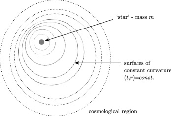
Figure 1: The surfaces $(t,r)$ are spheres, which are concentric to leading order in $\delta$ in both the exterior and interior limits.

With this choice of coordinates, the local energy density of the dust separates uniquely into a spherical symmetric part, $\varepsilon_{s}$, and and a non-spherical part, $\varepsilon_{ns}$:

$$\varepsilon=\varepsilon_{s}(t,R)+\varepsilon_{ns}(t,R,\theta,\varphi),$$

where:

$$\kappa\varepsilon_{s} = \frac{2M_{,R}}{R^{2}},$$ (7)

$$\kappa\varepsilon_{ns} = -\frac{R\nu_{,R}}{1+\nu_{,R}R}\cdot\left(\frac{2M}{R^{3}}\right)_{,R}.$$ (8)

We define $M_{,R}=M_{,r}/R_{,r}$. Following the conventions of our previous paper we write define

$$M:=m+Z(r),$$

where $m$ is the gravitational mass of our ‘star’.

III.1 Exterior Expansion

As a result of the way that the inhomogeneity is introduced in these models, we want the FRW limit to be ‘natural’ , that is for the $O(3)$ orbits to become concentric in this limit; we therefore require $\nu_{r}\sim o(1)$ as $\delta\rightarrow 0$ in the exterior. This follows from the requirement that the whole spacetime should become homogeneous in a smooth fashion in the limit where the mass of our ‘star’ vanishes: $m\rightarrow 0$. Put another way, the introduction of our star is the only thing responsible for making the surfaces of constant curvature non-concentric. We define, as in the previous paper, dimensionless ‘radial’ and time coordinates appropriate for the exterior by

$$\tau=H_{0}t,\text{ \ \ }\rho=H_{0}r.$$

The exterior limit is defined by $\delta\rightarrow 0$ with $\tau$ and $\rho$ fixed. In the exterior region we find asymptotic expansions in this limit. According to our prescription, we write

$$H_{0}Z(\rho)\sim\frac{1}{2}\Omega_{m}\rho^{3}+\delta^{p}z_{1}(r)+o(\delta^{p}),$$

and

$$H_{0}^{-1}\lambda_{i}\sim\delta^{s}l_{i}(\rho)+\mathcal{o}(\delta^{s}).$$

Since $H_{0}^{-2}\left(\frac{2M}{R^{3}}\right)_{,R}\sim\mathcal{O}(\delta^{p},\delta)$, we have that: $H_{0}^{-2}\kappa\varepsilon_{ns}\sim\mathcal{O}(\delta^{p+s},\delta^{1+s})$ whereas $H_{0}^{-2}\kappa\varepsilon_{s}\sim\mathcal{O}(\delta^{p},\delta)$. Thus, the non-spherical perturbation to the energy density is always of subleading order compared to the first order in spherical perturbation. The first-order, non-spherical, metric perturbation appears at $\mathcal{O}(\delta^{s})$; however, since this is equivalent to a coordinate transform on $(r,\theta,\varphi)$ and the dilaton field, $\phi$, is homogeneous to leading order in the exterior, this perturbation does not make any corrections to the dilaton conservation equation at $\mathcal{O}(\delta^{s})$. Thus, both at leading order, and at next-to-leading order, both the energy density and the dilaton field will behave in the same way as in the spherically-symmetric Tolman-Bondi case - with the possible addition of a non-spherically symmetric vacuum perturbation to the dilaton, $\phi$, i.e. $\phi\sim\phi_{s}+\phi_{ns}+o(\delta^{p})$ where $\phi_{s}$ is the spherically symmetric solution and $\square_{FRW}\phi_{ns}=0$. As in our previous paper, however, we are not especially interested in the exterior solution for $\phi$ beyond zeroth order, just the effect of any background variation in $\phi$ on what is measured on the surface of a local ’star’.

III.2 Interior Expansion

We define dimensionless coordinates for the interior in the same way as we did for the spherically symmetric case:

$$T=L_{I}^{-1}(t-t_{0})\text{ and }\xi=R/R_{s}.$$

We define the interior limit to be $\delta\rightarrow 0$ with $T$ and $\xi$ fixed, and perform out interior asymptotic expansions in this limit. To lowest order in the interior region, we write $Z\sim\delta^{q}R_{s}\mu_{1}$, and $\lambda_{i}:=\delta_{q^{\prime}}R_{s}^{-1}b_{i}$, where $i=\{x,y,z\}$. The condition that $\kappa\varepsilon>0$ everywhere requires $q^{\prime}\geq q$ and then, to next-to-leading order, the interior expansion of $\phi$ will be the same as it was in the spherically-symmetric Tolman-Bondi case. We can potentially include a non-spherical vacuum component for $\phi$; however, this will be entirely determined by a boundary condition on $R=R_{s}$ and the need that it should vanish for large $R$. To find the leading-order behaviour of the $\phi_{,T}$ we need to know $\phi$ at next-to-leading order. The only new case we need to consider therefore is when $q^{\prime}=q$, i.e. $\kappa\varepsilon_{ns}\sim\kappa\varepsilon_{s}$. In the spherically symmetric case we considered two distinct subclasses of the Tolman-Bondi models: the flat, $k=0$, Gautreau-Tolman-Bondi spacetimes, gautreau ; kras and the non-flat, $k\neq 0$, Tolman-Bondi models with a simultaneous initial singularity. In Gautreau-Tolman-Bondi models the initial singularity is non-simultaneous from the point of view of geodesic observers. The latter class is the more realistic, since in the former the world-lines of matter particles stream out of the surface of our star at $R=R_{s}|_{R=R_{s}}$ i.e. $R_{,t}>0$, whereas in the simultaneous big-bang models we can demand that matter particles fall onto this surface i.e. $R_{,t}|_{R=R_{s}}<0$. With this choice, and if $R_{s}=2m$, the non-flat models properly describe the embedding of a black hole into an expanding universe, whereas the Gautreau-Tolman-Bondi model technically describes the embedding of a white-hole in the same universe. In this paper we shall, therefore, only give the results explicitly for the non-flat case – however, we can present a simple procedure to transform our results to the flat Gautreau case.

We define  

$$\eta=\left(\xi^{3/2}-3T/2\right)^{2/3};\text{ }R_{s}\eta=r+\mathcal{O}(\delta^{q},\delta^{2/3}).$$

From the exact solutions we find:

$$k(\eta)=\delta^{2/3}k_{0}\left(1+\delta^{q}\mu_{1}(\eta)+o\left(\delta^{q}\right)\right)+\mathcal{O}\left(\delta^{5/3}\right),$$

where

$$k_{0}(\delta T)=\frac{2m}{R_{s}}\left(\frac{\pi}{H_{0}t_{0}+\delta T}\right)^{2/3}.$$

We can remove the $\mathcal{O}(\delta^{2/3})$ metric perturbation by a redefinition of the $T$ coordinate, $T\rightarrow T^{\ast}$:

$$\sqrt{1-\delta^{2/3}k_{0}}T^{\ast}=T+\int^{\xi}\frac{\sqrt{\frac{2m}{R_{s}\xi^{\prime}}}\left(1-\sqrt{1-\left(\frac{\delta^{2/3}\pi\xi^{\prime}}{H_{0}t_{0}+\delta T}\right)}\right)}{1-\frac{2m}{R_{s}\xi^{\prime}}}\mathrm{d}\xi^{\prime}.$$

To leading order we see that $T\sim T^{\ast}$. The interior expansion of the metric, for $q^{\prime}=q$, is written:

$$\mathrm{d}s_{int}^{2}\sim R_{s}^{2}\left(j_{ab}^{(0)}(\xi)+\delta^{q}j_{ab}^{(1)s}(\xi,\chi)+\delta^{q}j_{ab}^{(1)ns}(\xi,\chi)+o(\delta^{q})\right)\mathrm{d}x^{a}\mathrm{d}x^{b}+o(\delta^{q}).$$

where $j_{ab}^{(0)}$ and $j_{ab}^{(1)s}$ are given by:

$$j_{ab}^{(0)}\mathrm{d}x^{a}\mathrm{d}x^{b} = \frac{R_{s}}{2m}\mathrm{d}T^{\ast 2}-\left(\mathrm{d}\xi+\xi^{-1/2}\mathrm{d}T^{\ast}\right)^{2}-\xi^{2}\{\mathrm{d}\theta^{2}+\sin^{2}\theta\mathrm{d}\varphi^{2}\},$$ (9)

$$j_{ab}^{(1)s}\mathrm{d}x^{a}\mathrm{d}x^{b} = -\frac{\mu_{1}(\chi)}{\xi^{1/2}}\mathrm{d}\xi\mathrm{d}T^{\ast}-\frac{\mu_{1}(\chi)}{\xi}\mathrm{d}T^{\ast 2}.$$ (10)

These are the same as in the spherically symmetric case. The non-spherically symmetric perturbation is given by

$$j_{ab}^{(1)ns}\mathrm{d}x^{a}\mathrm{d}y^{b} = 2(b_{z}\cos\theta+b_{x}\cos\varphi\sin\theta+b_{y}\sin\varphi\sin\theta)\xi\mathrm{d}\eta^{2}$$

$$-2\xi^{2}\left[b_{z}\sin\theta+b_{x}\cos\varphi(1-\cos\theta)+b_{y}\sin\varphi(1-\cos\theta)\right]\mathrm{d}\theta\mathrm{d}\eta$$

$$-2\xi^{2}(1-\cos\theta)\sin\theta(b_{x}\sin\varphi-b_{y}\cos\varphi)\mathrm{d}\varphi\mathrm{d}\eta.$$

The spherically symmetric part of the local energy density, $\kappa\varepsilon_{s}$ is the same as it was in the Tolman-Bondi cases:

$$R_{s}^{2}\kappa\varepsilon_{s}=\delta^{q}\frac{2m}{R_{s}}\frac{\mu_{1,\xi}}{\xi^{3/2}\eta^{1/2}}.$$

The non-spherically symmetric part is:

$$R_{s}^{2}\kappa\varepsilon_{ns}=-\delta^{q}\frac{6m}{R_{s}}\frac{\left(b_{z}\cos\theta+b_{x}\sin\theta\cos\phi+b_{y}\sin\theta\sin\phi\right)}{\xi^{3/2}\eta^{1/2}}.$$

and to ensure that the energy density is everywhere positive we need $\mu_{,\eta}^{(1)}\geq 3b_{i}$.

IV Extension to quasi-spherical situations

IV.1 Boundary Conditions

We demand the same boundary conditions as before: as the physical radius tends to infinity, $R\rightarrow\infty$, we demand that the dilaton tends to its homogeneous cosmological value: $\phi(R,t)\rightarrow\phi_{c}(t)$. This can be applied to the exterior approximation. In the interior, we demand that the dilaton-flux passing out from the surface of our ‘star’ at $R=R_{s}$ is, at leading order, parametrised by:

$$-R_{s}^{2}\left(1-\frac{2m}{R_{s}}\right)\left.\partial_{\xi}\phi_{0}\right|_{\xi=R_{s}}=2mF\left(\bar{\phi}_{0}\right)=\int_{0}^{R_{s}}\mathrm{d}R^{\prime}R^{\prime}{}^{2}B_{,\phi}(\phi_{0}(\hat{\xi}^{\prime}))\kappa\varepsilon(R^{\prime}),$$ (12)

where $\bar{\phi}_{0}=\phi_{0}(R=R_{s})$. The function $F(\phi)$ can be found by solving the dilaton field equations to leading order in the $R<R_{s}$ region. If the interior region is a black-hole ($R_{s}=2m$) then we must have $F(\phi)=0$; otherwise we expect $F(\phi)\sim B_{,\phi}(\phi)$. Without considering the sub-leading order dilaton evolution inside our ‘star’, i.e. at $R<R_{s}$, we cannot rigorously specify any boundary conditions beyond leading order. Despite this, we can guess at a general boundary condition by perturbing eq. (12):

$$-R_{s}^{2}\left(1-\frac{2m}{R_{s}}\right)\left.\partial_{R}\tilde{\delta}(\phi)\right|_{\xi=R_{s}}=-\left.\tilde{\delta}\left(\sqrt{-g}g^{RR}\right)\partial_{R}\phi_{0}\right|_{R=R_{s}}+2\tilde{\delta}(M)F\left(\bar{\phi}_{0}\right)+2mF_{,\phi}(\bar{\phi}_{0})\tilde{\delta}\left(\bar{\phi}_{0}\right)+\mathrm{smaller}\;\mathrm{terms},$$ (13)

where $\tilde{\delta}(X)$ is the first sub-leading order term in the interior expansion of $X$; $M$ is the total mass contained inside $\xi<R_{s}$ and is found by requiring the conservation of energy; and at $t=t_{0}$ we have $M=m$. Only $\tilde{\delta}\left(\bar{\phi}_{0}\right)$ remains unknown; however, we shall assume it to be the same order as $\tilde{\delta}(\phi)$ and see that this unknown term is usually suppressed by a factor of $2m/R_{s}$ relative to the other terms in eq. (13).

IV.2 Interior Expansion

In the spherically symmetric case we found that $\phi\sim\phi_{I}^{(0)}+\delta^{q}\phi_{I}^{(1)}+o(\delta^{q})$. In the non-spherical case, where $q^{\prime}=q$, we relabel $\phi_{I}^{(1)}\rightarrow\phi_{I}^{(1)s}$ and we have additional non-spherical modes:

$$\phi\sim\phi_{I}^{(0)}(\xi,T)+\delta^{q}\phi_{I}^{(1)s}(\xi,T)+\delta^{q}\phi_{I}^{(1)z}(\xi,T)\cos\theta+\delta^{q}\phi_{I}^{(1)x}(\xi,T)\sin\theta\cos\varphi+\delta^{q}\phi_{I}^{(1)y}(\xi,T)\sin\theta\sin\varphi+o(\delta^{q})$$

where:

$$-\frac{2m}{R_{s}}\left(\xi^{3/2}\phi_{I,TT}^{(1)i}+\frac{3}{2}\phi_{I,T}^{(1)i}\right) + \frac{1}{\eta^{1/2}}\left(\frac{\xi^{5/2}}{\eta^{1/2}}\phi_{I,\eta}^{(1)i}\right)_{,\eta}-\frac{2}{\xi^{1/2}}\phi_{I}^{(1)i}=\frac{6m}{R_{s}}B_{,\phi}\left(\phi_{I}^{0}\right)\frac{b_{i}\left(\eta\right)}{\eta^{1/2}}$$

$$+ \left(\frac{2m}{R_{s}}\right)\frac{1}{\eta^{1/2}}F\left(\bar{\phi}_{0}\right)\left[\left(b_{i}(\eta)\xi\left(\frac{1+\frac{2m}{R_{s}\xi}}{1-\frac{2m}{R_{s}\xi}}\right)\right)_{,\eta}-2b_{i}(\eta)\right].$$

We can solve this order by order in $2m/R_{s},$ and to lowest order we find:

$$\phi_{I}^{(1)i} \sim \frac{2m}{R_{s}}B_{,\phi}\left(\phi_{I}^{0}\right)\xi\int^{\eta}\mathrm{d}\eta^{\prime}\frac{b_{i}(\eta^{\prime})}{\xi^{{}^{\prime}2}}-\frac{2m}{R_{s}}B_{,\phi}\left(\phi_{I}^{0}\right)\frac{1}{\xi^{2}}\int_{\xi=1}^{\eta}\mathrm{d}\eta^{\prime}\xi^{\prime}b_{i}(\eta^{\prime})$$

$$+ \frac{2m}{R_{s}}F\left(\bar{\phi}_{0}\right)\frac{1}{\xi^{2}}\int_{\xi=1}^{\eta}\mathrm{d}\eta^{\prime}b_{i}(\eta^{\prime})\xi^{\prime}+\frac{C_{i}}{\xi^{2}}+D_{i}\xi+\mathcal{O}((2m/R_{s})^{2})$$

Since we are interested in finding when and where the local time variation of $\phi$ deviates from its cosmological value, we are chiefly concerned with the case $q\leq 1$. The matching condition then requires that we fix $D_{i}$ so that in the intermediate limit we have $\phi_{I}^{(1)i}\sim\xi^{n}$ with $n<1$. The value of $C_{i}$ should be set by a boundary condition on $R=R_{s}$. We cannot specify $C_{i}$ exactly without further information about the interior of our ‘star’ in $R<R_{s}$. If we assume that the prescription for the sub-leading order boundary condition given above is correct then we find:

$$\partial_{\xi}\phi_{I}^{(1)i}|_{\xi=1} \sim \frac{2m}{R_{s}}\left.\frac{b_{i}}{\eta^{1/2}}\right|_{\xi=1}F\left(\bar{\phi}_{0}\right)+\mathcal{O}((2m/R_{s})^{2})$$

$$\Rightarrow C_{i} = \frac{m}{R_{s}}B_{,\phi}\left(\phi_{I}^{0}\right)\int^{\xi=1}\mathrm{d}\eta^{\prime}\frac{b_{i}(\eta^{\prime})}{\xi^{{}^{\prime}2}}+\tfrac{1}{2}D$$

From now onwards we set $C_{i}=0,$ for simplicity; even when this is not correct we do not expect the magnitude of $C_{i}$ or $C_{i,T}$ to be larger than any of the other terms in $\phi_{I}^{(1)i}$ or $\phi_{I,T}^{(1)i}$, respectively. The time-derivative of $\phi_{I}^{(1)i}$ for fixed $R$ is:

$$\phi_{I,T}^{(1)i}\sim\frac{4m}{R_{s}}B_{,\phi}\left(\phi_{I}^{0}\right)\xi\int^{\eta}\mathrm{d}\xi^{\prime}\frac{b_{i}(\eta^{\prime})}{\xi^{{}^{\prime}5/2}}+\frac{2m}{R_{s}}B_{,\phi}\left(\phi_{I}^{0}\right)\frac{1}{\xi^{2}}\int_{\xi=1}^{\eta}\mathrm{d}\xi^{\prime}\frac{b_{i}(\eta^{\prime})}{\xi^{1/2}}-\frac{2m}{R_{s}}F\left(\bar{\phi}_{0}\right)\frac{1}{\xi^{2}}\int_{\xi=1}^{\eta}\mathrm{d}\eta^{\prime}\frac{b_{i}(\eta^{\prime})}{\xi^{1/2}}+D_{,T}\xi$$ (16)

In the next section we shall discuss what we require of the $b_{i}$ for the matching procedure to be valid. In section VI we will then use the matching conditions to find $D$ and $D_{,T}$.

We could also relax the requirement that the leading-order mode in $\phi$ be spherically symmetric. At next-to-leading order these new modes would generate extra terms in $\phi_{I}^{(1)}$. In general, an $l$-pole at leading order becomes an $l+1$-pole at next-to-leading order. The magnitude of the extra time-dependence that is picked up is, however, the same each time. Hence, we restrict ourselves by taking the leading-order mode to be spherically symmetric for the time being. Note also that we can pass from the simultaneous big-bang case, to the spatially flat, ‘Gautreau’, case by setting $k=0$ and making the transform $\eta\rightarrow\chi=\left(\xi^{3/2}+3T/2\right)^{2/3}$. This will also mean that $\phi_{I,T}\rightarrow-\phi_{I,T}$.

V Validity of Approximations

All of the conditions found in Paper I for the matching of the spherically symmetric parts of $\phi$ to be possible still apply here. However, we must now satisfy some extra conditions that come from the requirement that the non-spherical parts should also be matchable.

We assume that $b_{i}\left(\eta\right)\propto\eta^{d_{i}}$ as $\eta\rightarrow\infty$ for some $d_{i}>0$. At order $\delta^{q}$, the growing mode in the non-spherically symmetric part of the interior approximation will then grow like $\delta^{q}\eta^{d_{i}+1}/\xi$. In the intermediate, or matching, region we have that $\eta,\xi\sim\delta^{-\alpha}$ for some $\alpha\in(0,1)$. We require $\phi_{I}$ to have a valid asymptotic expansion this region. This implies that there exists some $\alpha\in(0,1)$ such that, for each $i$, we have $\alpha-q/d_{i}>0$.

In the exterior we shall write $H_{0}^{-1}\lambda_{i}\sim\delta^{p_{i}^{\prime}}l_{i}(\rho)$, where $p_{i}^{\prime}>0$ comes from the requirement that the 2-spheres of constant curvature become concentric in the exterior limit. As $\rho\rightarrow 0$ we assume that $l_{i}(\rho)\propto\rho^{-f_{i}}$. We previously stated that $Z\sim\frac{1}{2}\Omega_{m}\rho^{3}+\delta^{p}z_{1}+o(\delta^{p})$ in the exterior. We assume that as $\rho\rightarrow 0$, we have $z_{1}\propto\rho^{-m}$. Although we did not explicitly consider the exterior expansion of $\phi$ we can now examine the behaviour of the leading-order non-spherically symmetric mode in the intermediate limit of that exterior expansion. We noted above that there will be no $\mathcal{O}(\delta^{p_{i}^{\prime}})$ correction resulting from the $l_{i}$. The leading-order mode will therefore either go like $\max_{i}\left(\delta^{p+p_{i}^{\prime}}z_{1}(\rho)l_{i}(\rho)\right)$ if $p<1$ or $\max_{i}\left(\delta^{1+p_{i}^{\prime}}(\rho)l_{i}(\rho)\right)$ otherwise, and $\rho\sim\mathcal{O}(\delta^{1-\alpha})$ in the intermediate region. For the exterior expansion to be valid in the intermediate region we therefore require

$$\max_{i}(p_{i}^{\prime} + (1-\alpha)(f_{i}+m))>-p\;\mathrm{if}\;p\leq 1,$$

$$\max_{i}(p_{i}^{\prime} + (1-\alpha)f_{i})>-1\;\mathrm{if}\;p\geq 1.$$

These conditions on $\alpha$ are equivalent to the following: there exists $\alpha$ such that the interior expansion of $R^{2}\kappa\varepsilon_{ns}$ is $o(1)$ as $\delta\rightarrow 0$ for all $0<\alpha^{\prime}<\alpha$ where $\xi,T\sim\mathcal{O}(\delta^{-\alpha})$, and the exterior expansion of $R^{2}\kappa\varepsilon_{ns}$ is also $o(1)$ as $\delta\rightarrow 0$ for all $0<\alpha^{\prime\prime}<\alpha$ where $\rho,\tau-\tau_{0}\sim\mathcal{O}(\delta^{1-\alpha})$. This suggests that the condition for the matching procedure to work, as far as the spherically non-symmetric modes are concerned, is simply that

$$R^{2}\kappa\varepsilon_{ns}\ll 1\;\mathrm{everywhere.}$$

We can also rephrase and generalise the conditions for the matching procedure to be possible w.r.t. the spherically symmetric modes (as found in shawbarrow1 ) in a similar fashion: for all $\alpha\in(0,1)$, and keeping $L_{I}^{\alpha}L_{E}^{1-\alpha}(t-t_{0}),L_{I}^{\alpha}L_{E}^{1-\alpha}R$ fixed, we have $\lim_{\delta\rightarrow 0}{R^{2}\kappa\Delta\varepsilon_{s}}=o(1)$ and $\lim_{\delta\rightarrow 0}{2(m+Z)/R}=o(1)$. We can combine our two conditions by simply replacing $\Delta\varepsilon_{s}$ by $\Delta\varepsilon$ in the above expression. Strictly speaking, since $\alpha\in(0,1)$ (as opposed to $[0,1)$, $(0,1]$ or $[0,1]$) we can also replace $\Delta\varepsilon$ by just $\varepsilon$ since $R^{2}\kappa\varepsilon_{FRW}$ is small everywhere outside the exterior region. For Szekeres backgrounds the first of these conditions implies the second everywhere outside the interior region. Therefore, the matching procedure is certainly possible to zeroth order, if:

$$\forall\alpha\in(0,1):\;\;\lim_{\delta\rightarrow 0}\left(R^{2}\kappa\varepsilon(R,t)\right)=o(1)\;\mathrm{and}\;\;\lim_{\delta\rightarrow 0}\left(M(R,t)/R\right)=o(1)\;\;\mathrm{with}\;\;\{L_{I}^{\alpha}L_{E}^{1-\alpha}(t-t_{0}),L_{I}^{\alpha}L_{E}^{1-\alpha}R\}\;\mathrm{fixed},$$

where $M(R,t)$ is the gravitational mass inside the surface $(t,R)=const$. Equivalently, in any intermediate region the background spacetime is asymptotically Minkowski as $\delta\rightarrow 0$: everywhere which is not in either the interior or exterior regions can be considered to be a weak-field perturbation of Minkowski spacetime. The power of our method is that we do not require this to be true of the interior and exterior regions. So long as this condition holds in the intermediate region, we can match the zeroth-order approximations in some region and find the circumstances under which condition (1) holds by comparing the relative sizes of the derivatives $\phi_{c,t}$ and $\phi_{I,t}^{(1)}$.

VI Matching

We rewrite the expression for the $\phi_{I}^{(1)i}$ in terms of the non-spherical part of local density:

$$\delta^{q}\phi_{I}^{(1)ns} = \delta^{q}\left(\phi_{I,t}^{(1)z}\cos\theta+\phi_{I,t}^{(1)x}\sin\theta\cos\varphi+\phi_{I,t}^{(1)y}\sin\theta\sin\varphi\right)$$

$$\sim -\frac{1}{3}B_{,\phi}\left(\phi_{I}^{0}\right)R\int^{r}\mathrm{d}r^{\prime}R_{,r}\kappa\varepsilon_{ns}(r^{\prime},t)-\frac{R}{R_{s}}\hat{D}(T,\theta,\phi)$$

$$-\frac{1}{3}B_{,\phi}\left(\phi_{I}^{0}\right)\frac{1}{R^{2}}\int_{R=R_{s}}^{r}\mathrm{d}r^{\prime}R_{,r}R^{3}\kappa\varepsilon_{ns}(r^{\prime},t)-\frac{1}{3}F\left(\bar{\phi}_{0}\right)\frac{1}{R^{2}}\int_{R=R_{s}}^{r}\mathrm{d}r^{\prime}R_{,r}R^{3}\kappa\varepsilon_{ns}(r^{\prime},t)$$

where $\hat{D}(T,\theta,\phi):=D_{z}\cos\theta+D_{x}\sin\theta\cos\varphi+D_{y}\sin\theta\sin\varphi$. By examining the dilaton equations of motion in the FRW region, we can see there is a component of the leading-order $(\theta,\varphi)$-dependent term in the exterior expansion or $\phi$ behaves like

$$-\frac{1}{3}B_{,\phi}(\phi_{c})R\int_{\infty}^{r}\mathrm{d}r^{\prime}R_{,r}\kappa\varepsilon_{ns}(r^{\prime},t)$$

for $R\ll H_{0}^{-1}$ and $t$ fixed. Therefore matching requires that we choose $\hat{D}$ such that

$$\delta^{q}\phi_{I}^{(1)ns} = \delta^{q}\left(\phi_{I,t}^{(1)z}\cos\theta+\phi_{I,t}^{(1)x}\sin\theta\cos\varphi+\phi_{I,t}^{(1)y}\sin\theta\sin\varphi\right)$$ (17)

$$\sim -\frac{1}{3}B_{,\phi}\left(\phi_{I}^{0}\right)R\int_{\infty}^{r}\mathrm{d}r^{\prime}R_{,r}\kappa\varepsilon_{ns}(r^{\prime},t)+\frac{1}{3}B_{,\phi}\left(\phi_{I}^{0}\right)\frac{1}{R^{2}}\int_{R=R_{s}}^{r}\mathrm{d}r^{\prime}R_{,r}R^{3}\kappa\varepsilon_{ns}(r^{\prime},t)$$

$$-\frac{1}{3}F\left(\bar{\phi}_{0}\right)\frac{1}{R^{2}}\int_{R=R_{s}}^{r}\mathrm{d}r^{\prime}R_{,r}R^{3}\kappa\varepsilon_{ns}(r^{\prime},t).$$

The interior expansion is now fully specified to order $\mathcal{O}(\delta^{p})$. We are interested in the behaviour of $\phi_{I,t}$ and we find

$$\delta^{q}\phi_{I,t}^{(1)ns} \sim \frac{2}{3}B_{,\phi}\left(\phi_{I}^{0}\right)R\int_{\infty}^{r}\mathrm{d}r^{\prime}R_{,r}R_{,t}\frac{\kappa\varepsilon_{ns}(r^{\prime},t)}{R}+\frac{1}{3}B_{,\phi}\left(\phi_{I}^{0}\right)\frac{1}{R^{2}}\int_{R=R_{s}}^{r}\mathrm{d}r^{\prime}R_{,r}R_{,t}R^{2}\kappa\varepsilon_{ns}(r^{\prime},t)$$

$$-\frac{1}{3}F\left(\bar{\phi}_{0}\right)\frac{1}{R^{2}}\int_{R=R_{s}}^{r}\mathrm{d}r^{\prime}R_{,r}R_{,t}R^{3}\kappa\varepsilon_{ns}(r^{\prime},t)+\frac{1}{3}F\left(\bar{\phi}_{0}\right)RR_{,t}\kappa\varepsilon_{ns}(r,t).$$

This expression is valid whenever $R_{s}\gg 2m$, and the requirements for matching are satisfied. In these cases we expect $F\left(\bar{\phi}_{0}\right)\approx B_{,\phi}\left(\phi_{I}^{0}\right)+\mathcal{O}(2m/R_{s})$; so, approximately, we have

$$\delta^{q}\phi_{I,t}^{(1)ns}\sim\frac{2}{3}B_{,\phi}\left(\phi_{c}\right)R\int_{\infty}^{r}\mathrm{d}r^{\prime}R_{,r}R_{,t}\frac{\kappa\varepsilon_{ns}(r^{\prime},t)}{R}+\frac{1}{3}B_{,\phi}\left(\phi_{c}\right)RR_{,t}\kappa\varepsilon_{ns}(r,t).$$

In the case, where $R_{s}=2m,$ and our ‘star’ is actually a black-hole, we require $F\left(\bar{\phi}_{0}\right)$ to ensure that the $\phi$ is well-defined as $R\rightarrow 2m$. Even so, in this case, equation (16) will not be strictly valid, since it was derived under the assumption of $R_{s}\gg 2m$. By inspection of the dilaton evolution equation in the interior, eq. (IV.2), however, we expect that $\delta^{q}\phi_{I,t}^{(1)ns}$ near the black-hole horizon to be of similar magnitude to the RHS of eq. (16).

Combining the results of this paper with those for the spherically symmetric case we find:

$$\phi_{I,t}-\phi_{c,t}\sim B_{,\phi}\left(\phi_{c}\right)\int_{\infty}^{r}\mathrm{d}r^{\prime}R_{,r}R_{,t}\kappa\Delta\varepsilon_{s}(r^{\prime},t)+\frac{2}{3}B_{,\phi}\left(\phi_{c}\right)R\int_{\infty}^{r}\mathrm{d}r^{\prime}R_{,r}R_{,t}\frac{\kappa\varepsilon_{ns}(r^{\prime},t)}{R}+\frac{1}{3}B_{,\phi}\left(\phi_{c}\right)RR_{,t}\kappa\varepsilon_{ns}(r,t).$$

We require that $|(\phi_{I,t}-\phi_{c,t})/\phi_{c,t}|\ll 1$ for 1 to hold and so ensure that local observations will detect variations of $\phi$ occurring on cosmological scales.

VII Generalisation: a conjecture

So far, we have found an analytic approximation to the values of $\phi$ and $\phi_{c,t}$ in the interior. More succinctly (although less explicitly) we can say that, to leading order in $\delta$, the values of $\phi$, $\phi_{,t}$ and $\phi_{,r}$ can all be found everywhere outside the exterior region from the approximation:

$$\phi\approx\phi_{hom}(t)+\phi_{l}(\vec{x},t),$$ (20)

where $\phi_{l}$ is the solution to:

$$\square_{sch}\phi_{l}=B_{,\phi}\kappa\Delta\varepsilon$$

with $\Delta\varepsilon=\varepsilon(\vec{x},t)-\varepsilon_{c}(t)$, $\square_{sch}$ is the wave operator in a Schwarzschild background, and $t$ is the proper time of a comoving observer. This is solved w.r.t. the boundary conditions $\phi_{l}\rightarrow 0$ as $R\rightarrow\infty$ (where $R=0$ is the centre of our ‘star’) and the flux out of the ‘star’ is as given by equations (12) and (13). The homogeneous term is

$$\phi_{hom}(t)=\phi_{c}(t+\Delta t(\vec{x},x))$$

where the lag, $\Delta t(\vec{x},t)$, is defined by:

$$\vec{\nabla}^{2}\Delta t-\vec{v}^{\ast}\cdot\vec{\nabla}(\vec{v}^{\ast}\cdot\vec{\nabla}\Delta t)-\vec{v}^{\ast}\cdot\vec{\nabla}\Delta t(\vec{\nabla}\cdot\vec{v}^{\ast})=-\vec{\nabla}\cdot\Delta\vec{v},$$

with $\nabla_{i}=\partial_{i}$, $i=\{1,2,3\}$, and $\Delta v=\vec{v}-H\vec{x}$, where $\vec{v}$ is the velocity of the dust particles relative to $R=\|\vec{x}\|=0$. The velocity $\vec{v}^{\ast}$ has the following properties: $\vec{v}^{\ast}=\vec{v}$ in some region that includes all the interior and excludes all of the exterior; $\vec{v}^{\ast}=\Delta\vec{v}$ everywhere else. In a general sense, the interior and exterior are two disjoint regions of total spacetimes where general-relativistic effects are non-negligible at leading order (e.g. such as when $\|\vec{v}\|\approx 1$). The interior region should be closed, and in the exterior region $\|\Delta\vec{v}\|$ is small. So, $\vec{v}^{\ast}$ should be defined in such a way that it respects all the symmetries of the spacetime and so that $\|\vec{v}^{ast}\|\ll 1$ everywhere outside the interior region. This is required to ensure that $\Delta t$, as defined above, is finite. It can be seen to come out of the matching procedure. When the background spacetime satisfies the conditions given below, the precise way in which $\vec{v}^{\ast}$ is defined does not effect the leading order behavior of $\Delta t$. For boundary conditions, we must require the flux out of $\Delta t$ out of the ‘star’ to vanish, and require $\Delta t\rightarrow 0$ as $\Delta v\rightarrow 0$, i.e. as $R\rightarrow\infty$. This is the natural generalisation of what has been seen in the Szekeres-Szafron backgrounds $\vec{v}^{i}=R_{,t}(R,t)\delta_{R}^{i}$. In these cases the equation is just an ordinary differential equation in $R$ with solution:

$$\Delta t=\int_{R}^{A}\mathrm{d}R^{\prime}\frac{(R_{,t}(R^{\prime},t)-HR^{\prime}+R_{,t}(R_{s},t)+HR_{s})}{1-R_{,t}^{2}(R^{\prime},t)}+\int_{A}^{\infty}\mathrm{d}R^{\prime}\frac{(R_{,t}(R^{\prime},t)-HR^{\prime}+R_{,t}(R_{s},t)+HR_{s})}{1-(R_{,t}(R^{\prime},t)-HR)^{2}},$$

where $A$ is some arbitrary value of $A$ in the intermediate region, and each $A$ represents a particular choice of definition for $\vec{v}^{\ast}$. This expression is only valid to leading order in the interior and intermediate regions. To this order all choices for $A$ are equivalent. Near $R=R_{s}$, to leading order in $\delta=L_{I}/L_{E}$, this ensures that $\mathrm{d}(t+\Delta t)\sim\mathrm{d}v$, where $v=t_{sch}+R+2m\ln(R/2m-1)$ is the advanced time coordinate and $t_{sch}$ is the standard, curvature-defined, Schwarzschild time-coordinate. The solution for $\phi_{hom}$ is then, to leading order in $\delta$, just the particular one given by Jacobson in jacobson . We have assumed that the generalisations of the Szekeres-Szafron result for $\phi$ hold. We have only proved that this assumption holds for the subset of Szekeres-Szafron spacetimes for which the matching procedure works. Nonetheless, based on this analysis, we conjecture that 20 provides a good numerical approximation to the value of $\phi$, and by differentiating once, to $\phi_{,t}$ and $\partial_{i}\phi$, $i=\{1,2,3\}$, near the surface of our ‘star’, for any dust plus $\Lambda$ spacetime that can be everywhere considered to be a weak-field perturbation of either Schwarzschild, Minkowski, or FRW spacetime; that is,

$$R^{2}\kappa\Delta\varepsilon(R,t)\ll 1,\qquad 2(M(R,t)-m)/R\ll 1$$

where $M(R,t)$ is the gravitational mass contained inside the surface $(R,t)=const$. One could seek to motivate our conjecture as some sort of analytical continuation from the Szekeres-Szafron spacetimes to more general backgrounds, but such arguments would, we believe, be hard to frame in any rigorous context and are beyond the scope of the analysis in this paper.

VIII Discussion

In this paper we have extended the analysis of shawbarrow1 to include a class of dust-filled spacetimes without any symmetries provided by the Szekeres-Szafron metrics. Again, we have used the method of matched asymptotic expansions to link the evolution of the dilaton field, $\phi$, in an approximately Schwarzschild region of spacetime to its evolution in the cosmological background. By these methods, we have provided a rigorous construction of what has been simply assumed about the matching procedures in earlier studies early . We have also analysed, more fully, the conditions that we need the background spacetime to satisfy for the matching procedure to be valid, and we have interpreted these conditions in terms of their requirements on the local energy density. Finally, we have conjectured a generalisation of our result to more general spacetime backgrounds than those considered here.

By combining the results found here with those of the previous paper, we conclude that, in the class of quasi-spherical Szekeres spacetimes in which the matching procedure is valid, the local time variation of the dilaton field will track its cosmological value whenever:

$$\left|\frac{B_{,\phi}\left(\phi_{c}\right)\int_{\infty}^{r}\mathrm{d}r^{\prime}R_{,r}\kappa\Delta(R_{,t}\varepsilon_{s}(r^{\prime},t))+\frac{2}{3}B_{,\phi}\left(\phi_{c}\right)R\int_{\infty}^{r}\mathrm{d}r^{\prime}R_{,r}R_{,t}\frac{\kappa\varepsilon_{ns}(r^{\prime},t)}{R}+\frac{1}{3}B_{,\phi}\left(\phi_{c}\right)RR_{,t}\kappa\varepsilon_{ns}(r,t)}{\dot{\phi}_{c}}\right|\ll 1.$$ (21)

When the cosmological evolution of $\phi$ is dominated by its matter coupling: $\dot{\phi}_{c}\sim\mathcal{O}(B_{,\phi}H_{0}^{-1}\kappa\varepsilon_{c}),$ this condition is equivalent to:

$$\left|H_{0}\int_{\infty}^{r}\mathrm{d}r^{\prime}R_{,r}\frac{\Delta(R_{,t}\varepsilon_{s}(r^{\prime},t))}{\varepsilon_{c}(t)}+\frac{2}{3}H_{0}R\int_{\infty}^{r}\mathrm{d}r^{\prime}R_{,r}R_{,t}R^{-1}\frac{\varepsilon_{ns}(r^{\prime},t)}{\varepsilon_{c}(t)}+\frac{1}{3}H_{0}R_{,t}\frac{\varepsilon_{ns}(r,t)}{\varepsilon_{c}(t)}\right|\ll 1.$$

In the other extreme, when the potential term dominates the cosmic dilaton evolution, the left-hand side of the above condition is further suppressed by a factor of $B_{,\phi}(\phi_{c})/V_{,\phi}(\phi_{c})\ll 1$. As in our previous paper, shawbarrow1 , we can see that for a given evolution of the background matter density, condition (1) is more likely to hold (or will hold more strongly) when $\left|B_{,\phi}(\phi_{c})\kappa\varepsilon_{c}/V_{,\phi}(\phi_{c})\right|\ll 1$. We reiterate our previous statement that: domination by the potential term in the cosmic evolution of the dilaton has a homogenising effect on the time variation of $\phi$.

The non-spherically symmetric parts of energy density enter into the expression differently. The magnitude of the terms on the left-hand side of eq. (21) is, as in the spherically symmetric case, still $\left\langle H_{0}R\Delta R_{,t}\varepsilon/\varepsilon\right\rangle(R,t)$ where $\left\langle\cdot\right\rangle(R,t)$ represents some ‘average’ over the region outside the surface $(R,t)=const$. We should note that, given the condition on $\kappa\varepsilon$ that has been required for matching, the leading-order contribution to $\kappa\varepsilon_{ns}$ is everywhere of dipole form and this is responsible for the special form of the average over the non-spherically symmetric terms. We can also see that, as a result of form of eqn. (21), peaks in $\kappa\varepsilon_{ns}$ that occur outside of the interior region will, in the interior, produce a weaker contribution to the left-hand side of eqn. (21) than a peak of similar amplitude in a spherically symmetric energy density $\kappa\varepsilon_{s}$. This behaviour would continue if we were also to account for higher multipole terms in $\kappa\varepsilon_{ns}$. The higher the multipole, the more ‘massive’ the mode, and the faster it dissipates.

If we are interested in finding a sufficient condition (as opposed to a necessary and sufficient one) for (1) to hold locally, then in most circumstances we will be justified in averaging over the non-spherically symmetric modes in the same way as we average over the spherically symmetric ones. In most cases, this will over-estimate rather than under-estimate the magnitude of the left-hand side of our condition, (21). This reasoning leads us to the statement that for $\dot{\phi}(\mathbf{x},t)\approx\dot{\phi}_{c}(t)$ to hold locally it is sufficient that:

$$\mathcal{I}:=\int_{\gamma(R)}\mathrm{d}lH_{0}R^{\prime}\frac{\Delta(v\varepsilon)}{\varepsilon_{c}}\ll 1$$ (22)

where $\mathrm{d}l:=\mathrm{d}rR_{,r}$, $v=R_{,t}$ is the velocity of the dust particles, $\lim_{R\rightarrow\infty}v=H_{0}R$. We make the same generalisation that we did in Paper I by taking $\gamma(R)$ to run from $R$ to spatial infinity along a past, radially-directed light-ray. In this way, we incorporate the limitations imposed by causality. We should also assume that the above expression includes some sort of average over angular directions; to be safe we could replace $\varepsilon$ by its maximum value for fixed $R$ and $t$. This sufficient condition, (22), is precisely the generalised condition proposed in our first paper on this issue. The inclusion of deviations from spherical symmetry, therefore, has little effect of the qualitative nature of the conclusions that were found in shawbarrow1 . If anything, we have seen that the non-spherical modes dissipate faster and, as a result, will produce smaller than otherwise expected deviations in the local time derivative of $\phi$ from the cosmological ones.

On Earth we should expect, as before, that the leading-order deviation of $\dot{\phi}$ from $\dot{\phi}_{c}$ is produced by the galaxy cluster in which we sit, and that for a dilaton evolution that is dominated by its coupling to matter, this effect gives $\mathcal{I}\approx 6\times 10^{-3}\Omega_{m}^{-1}h\ll 1$, where $\Omega_{m}\approx 0.27$ and $h\approx 0.71$. If the cosmic dilaton evolution is potential dominated then $\mathcal{I}$ is even smaller. We conclude, as before, that irrespective of the value of the dilaton-to-matter coupling, and what dominates the cosmic dilaton evolution, that

$$\dot{\phi}(\mathbf{x},t)\approx\dot{\phi}_{c}(t)$$

will hold in the solar system in general, and on Earth in particular, to a precision determined by our calculable constant $\mathcal{I}$. We also conclude, as before, that whenever $\mathcal{I}\ll 1$ near the horizon of a black hole, there will be no significant gravitational memory effect for physically reasonable values of the parameters memory ; jacobson .

Our result relies on one major assumption: the physically realistic condition that the scalar field should be weakly coupled to matter and gravity – in effect, the variations of ’constants’ on large scales must occur more slowly than the universe is expanding and so their dynamics have a negligible back-reaction on the cosmological background metric. In this paper we have removed the previous condition of spherical symmetry at least in as far as the spacetime background is well described by Szekeres-Szafron solution. We have therefore extended the domain of applicability our general proof: that terrestrial and solar system based observations can legitimately be used to constrain the cosmological time variation of supposed ‘constants’ of Nature and other light scalar fields.

References

- (1) J.K. Webb et al, Phys. Rev. Lett. 82, 884 (1999); M. T. Murphy et al, Mon. Not. Roy. Astron. Soc. 327, 1208 (2001); J.K. Webb et al, Phys. Rev. Lett. 87, 091301 (2001); M.T. Murphy, J.K. Webb and V.V. Flambaum, Mon. Not R. astron. Soc. 345, 609 (2003); H. Chand et al., Astron. Astrophys. 417, 853 (2004); R. Srianand et al., Phys. Rev. Lett. 92, 121302 (2004). J. Bahcall, C.L. Steinhardt, and D. Schlegel, Astrophys. J. 600, 520 (2004); R. Quast, D. Reimers and S.A Levshakov, A. & A. 386, 796 (2002). S.A. Levshakov, et al., A. & A. 434, 827 (2005); S.A. Levshakov, et al., astro-ph/0511765; G. Rocha, R. Trotta, C.J.A.P. Martins, A. Melchiorri, P.P. Avelino, R. Bean, and P.T.P. Viana, Mon. Not. astron. Soc. 352, 20 (2004); J. Darling, Phys. Rev. Lett. 91, 011301 (2003); J. Darling, Astrophys. J. 612, 58 (2004); M.J. Drinkwater, J.K. Webb, J.D. Barrow and V.V. Flambaum, Mon. Not. R. Astron. Soc. 295, 457 (1998); W. Ubachs and E. Reinhold, Phys. Rev. Lett. 92, 101302 (2004); R. Petitjean et al, Comptes Rendus Acad. Sci. (Paris) 5, 411 (2004); P. Tzanavaris, J.K. Webb, M.T. Murphy, V.V. Flambaum, and S.J. Curran, Phys. Rev. Lett. 95, 041301 (2005); B. Bertotti, L. Iess and P. Tortora, Nature 425, 374 (2003).
- (2) E.A. Milne, E. A. Milne, Relativity, Gravitation and World Structure, Clarendon, Oxford, (1935).
- (3) P.A.M. Dirac, Nature P.A.M. Dirac, Nature 139, 323 (1937).
- (4) G. Gamow, Phys. Rev. Lett. 19, 757 and 913 (1967).
- (5) J.D. Barrow and F.J. Tipler, The Anthropic Cosmological Principle, Oxford UP, Oxford (1986);
- (6) P. Jordan, Ann. Phys. 36, 64 (1939).
- (7) C. Brans and R.H. Dicke, Phys. Rev. 124, 925 (1961).
- (8) J.D. Bekenstein, Phys. Rev. D 25, 1527 (1982).
- (9) H. Sandvik, J.D. Barrow and J. Magueijo, Phys. Rev. Lett. 88, 031302 (2002); J. D. Barrow, H. B. Sandvik and J. Magueijo, Phys. Rev. D 65, 063504 (2002); J. D. Barrow, H. B. Sandvik and J. Magueijo, Phys. Rev. D 65, 123501 (2002); J. D. Barrow, J. Magueijo and H. B. Sandvik, Phys. Rev. D 66, 043515 (2002); J. Magueijo, J. D. Barrow and H. B. Sandvik, Phys. Lett. B 541, 201 (2002); H. Sandvik, J.D. Barrow and J. Magueijo, Phys. Lett. B 549, 284 (2002); J.D. Barrow, D. Kimberly and J. Magueijo, Class. Quantum Grav. 21, 4289 (2004).
- (10) D. Kimberly and J. Magueijo, Phys. Lett. B 584, 8 (2004); D. Shaw and J.D. Barrow, Phys. Rev. D 71, 063525 (2005); D. Shaw, Phys. Lett. B 632, 105 (2006).
- (11) J.D. Barrow and J. Magueijo, Phys. Rev. D 72, 043521 (2005); J.D. Barrow, Phys. Rev. D 71, 083520 (2005).
- (12) J.P. Uzan, Rev. Mod. Phys. J.P. Uzan, Rev. Mod. Phys. 75, 403 (2003): J.-P. Uzan, astro-ph/0409424. K.A. Olive and Y-Z. Qian, Physics Today, pp. 40-5 (Oct. 2004); J.D. Barrow, The Constants of Nature: from alpha to omega, (Vintage, London, 2002); J.D. Barrow, Phil. Trans. Roy. Soc. 363, 2139 (2005).
- (13) D. Shaw and J.D. Barrow, gr-qc/0512022.
- (14) T. Damour and A. Polyakov, Nucl. Phys. B 423, 532 (1994).
- (15) K.A. Olive and M. Pospelov, Phys. Rev. D 65, 085044 (2002); E. J. Copeland, N. J. Nunes and M. Pospelov, Phys. Rev. D 69, 023501 (2004); S. Lee, K.A. Olive and M. Pospelov, Phys. Rev. D 70, 083503 (2004); G. Dvali and M. Zaldarriaga, hep-ph/0108217; P.P. Avelino, C.J.A.P. Martins, and J.C.R.E. Oliveira, Phys. Rev. D 70 083506 (2004).
- (16) D. Shaw and J.D. Barrow, gr-qc/0512117.
- (17) P. Szekeres, Commun. Math. Phys. 41, 55 (1975)
- (18) D.A. Szafron, J. Math. Phys. 18, 1673 (1977); D.A. Szafron and J. Wainwright, J. Math. Phys. 18, 1668 (1977).
- (19) E. J. Hinch, Perturbation methods, (Cambridge UP, Cambridge, 1991); J. D. Cole, Perturbation methods in applied mathematics, (Blaisdell, Waltham, Mass., 1968).
- (20) W. L. Burke, J. Math. Phys. 12, 401 (1971); P. D. D’Eath, Phys. Rev. D. 11, 1387 (1975); P. D. D’Eath, Phys. Rev. D. 12, 2183 (1975).
- (21) D.A. Szafron and C.B. Collins, J. Math. Phys. 20, 2354 (1979).
- (22) A. Krasinski, Inhomogeneous Cosmological Models, (Cambridge UP, Cambridge, 1996).
- (23) W. Bonnor, Commun. Math. Phys. 51, 191 (1976).
- (24) J. D. Barrow and J. Stein-Schabes, Phys. Lett. 103A, 315 (1984); U. Debnath, S. Chakraborty, and J.D. Barrow, Gen. Rel. Gravitation 36, 231 (2004).
- (25) G. Lemaître, C. R. Acad. Sci. Paris 196, 903 & 1085 (1933)
- (26) R.C. Tolman, Proc. Nat. Acad. Sci. USA 20, 169 (1934); H. Bondi, Mon. Not. R. astron. Soc. 107, 410 (1947)
- (27) P. Szekeres, Phys. Rev. D 12, 2941 (1975).
- (28) R. Gautreau, Phys. Rev. D. 29, 198 (1984).
- (29) T. Jacobson, Phys. Rev. Lett. 83, 2699 (1999).
- (30) J.D. Barrow and C. O’Toole, Mon. Not. Roy. Astron. Soc. 322, 585 (2001); C. Wetterich, JCAP 10, 002 (2003); P.P. Avelino, C.J.A.P. Martins, J. Menezes, C. Santos, astro-ph/0512332.
- (31) J.D. Barrow, Phys. Rev. D 46, R3227 (1992); J.D. Barrow, Gen. Rel. Gravitation 26, 1 (1992); J.D. Barrow and B.J. Carr, Phys. Rev. D 54, 3920 (1996); H. Saida and J. Soda, Class. Quantum Gravity 17, 4967 (2000); J.D. Barrow and N. Sakai, Class. Quantum Gravity 18, 4717 (2001); T. Harada, C. Goymer and B. J. Carr, Phys. Rev. D. 66, 104023 (2002).