Abstract

In this paper we investigate the effects that an anomalous acceleration as that experienced by the Pioneer spacecraft after they passed the 20 AU threshold would induce on the orbital motions of the Solar System planets placed at heliocentric distances of 20 AU or larger as Uranus, Neptune and Pluto. It turns out that such an acceleration, with a magnitude of $8.74\times 10^{-10}$ m s^-2, would affect their orbits with secular and short-period signals large enough to be detected according to the latest published results by E.V. Pitjeva, even by considering errors up to 30 times larger than those released. The absence of such anomalous signatures in the latest data rules out the possibility that in the region 20-40 AU of the Solar System an anomalous force field inducing a constant and radial acceleration with those characteristics affects the motion of the major planets.

Keywords: Pioneer anomaly; celestial mechanics; ephemerides; outer planets of the Solar System

1 Introduction

The Pioneer 10/11 missions were the first spacecraft to explore the outer Solar System. Pioneer 10 was launched in March 1972; Pioneer 11 followed it in April 1973. After the encounters with Jupiter and Saturn, both Pioneer spacecraft continued to explore the outer regions of the Solar System following nearly ecliptical hyperbolic paths in opposite directions. The last successful communication with Pioneer 10 occurred in April 2002, at nearly 70 AU from our planet, while the last scientific observations were returned by Pioneer 11 in September 1995 when it was at approximately 40 AU from the Earth. The last attempt to communicate with Pioneer 10 was made on March 2006, but without success [2]. The so-called Pioneer anomaly consists in an anomalous constant and uniform acceleration directed towards the Sun of $(8.74\pm 1.33)\times 10^{-10}$ m s^-2 found in the data of both spacecraft from the moment when they passed the threshold of 20 AU [3, 4, 5]. Various attempts to explain this feature in terms of known physical and engineering effects have been done, but without success; the nature of the Pioneer anomaly is, at present, still unexplained. It is not clear if the anomaly is due to some internal systematic, as suggested, e.g., in [6], or has an external origin. Dedicated space missions have recently been proposed [7, 8], while the authors of [9] put forth two non-dedicated scenarios involving either a planetary exploration mission to the outer Solar System or a piggy-backed micro satellite to be launched toward Saturn or Jupiter.

In this paper we propose to analyze some aspects of the problem of the Pioneer anomaly. In particular, we will investigate the possibility that an external, unknown constant and uniform force field inducing an acceleration of $8.74\times 10^{-10}$ m s^-2 on a test particle is present in the outer regions of the Solar System within 20-40 AU. The outline of our approach is the following.

Let us consider a constant and uniform acceleration radially directed towards the Sun and of very small magnitude so that it can be treated with the usual perturbative approaches; we will deal with it from a purely phenomenological point of view, without making any speculation about its origin. For a review of many proposed mechanisms involving possible ‘new’ physics, see [10] and references therein. What is its impact on the orbital motion of the planets of the Solar System whose semimajor axis is larger than 20 AU like Uranus, Neptune and Pluto? it should be noted that, at present there are no data supporting a more gradual onset of such an anomalous effect, and in the framework of this simplified model such planets, due to their relatively small eccentricities ($e_{\rm Uranus}=0.047$, $e_{\rm Neptune}=0.008$ and $e_{\rm Pluto}=0.248$), would be acted upon by the anomalous acceleration in all portions of their orbits.

An analogous approach was recently followed by the authors of [11]. Contrary to us, they discard the possibility of using the major planets of the outer Solar System. The focus of [11] is on some selected minor bodies characterized by large semimajor axes and eccentricities like some unusual minor bodies, Trans-Neptunian Objects (TNOs) and Centaurs. However, such objects are not constantly under the action of the hypothetical anomalous acceleration under investigation because of their highly eccentric orbits ($0.620<e<0.947$). According to the authors of [11], a relatively low-cost future astrometric campaign should resolve the problem within the next twenty years. A different position about the outer planets can be found in [9]. Another recent paper in which a comparison between planetary observations and a theoretically derived quantity related to the Pioneer anomaly is attempted yielding similar conclusions is [12].

In our paper we first work out, both analytically and numerically, the orbital perturbations induced by a disturbing acceleration like the Pioneer one on the Keplerian orbital elements of a planet. We find that the semimajor axis, the eccentricity, the perihelion and the mean anomaly of a test particle are affected by short-periods signatures and the perihelion and the mean anomaly undergo also long-period, secular effects. Then, numerical simulations of the temporal evolutions of the directly observable right ascensions and declinations of the planets induced by a Pioneer-like acceleration are performed. Contrary to the position of the authors of [11] and in according to the conclusions of [9, 12], it turns out that the predicted anomalous effects of this kind would be sufficiently large to be well detected with the present-day level of accuracy in planetary orbit determination [14], even by considering errors considerably larger than those released. Their absence tell us that in the outer region of the Solar System within 20-40 AU there is no any unknown force field, with the characteristics of that experienced by the Pioneer spacecraft, which affects the motion of the major planets.

2 The Gauss rate equations

The Gauss equations for the variations of the semimajor axis $a$, the eccentricity $e$, the inclination $i$, the longitude of the ascending node $\Omega$, the argument of pericentre $\omega$ and the mean anomaly $\mathcal{M}$ of a test particle of mass $m$ in the gravitational field of a body $M$ can be derived quite generally from [15]

$$\ddot{\boldsymbol{r}}+{\frac{\mu}{r^{3}}}\boldsymbol{r}=\boldsymbol{A},$$ (1)

where $\mu=G(M+m)$ and $\boldsymbol{r}=\boldsymbol{r}_{m}-\boldsymbol{r}_{M}$. Eq. (1) holds for every perturbing acceleration $\boldsymbol{A}$, whatever its cause or size. The variations of the elements are, for an entirely radial acceleration

$$\frac{{{d}}{a}}{{{d}}{t}} = {\frac{2e}{n\sqrt{1-e^{2}}}}\ A_{r}\sin f,$$ (2)

$$\frac{{{d}}{e}}{{{d}}{t}} = {\frac{\sqrt{1-e^{2}}}{na}}\ A_{r}\sin f,$$ (3)

$$\frac{{{d}}{i}}{{{d}}{t}} = 0,$$ (4)

$$\frac{{{d}}{\Omega}}{{{d}}{t}} = 0,$$ (5)

$$\frac{{{d}}{\omega}}{{{d}}{t}} = -{\frac{\sqrt{1-e^{2}}}{nae}}\ A_{r}\cos f,$$ (6)

$$\frac{{{d}}{\mathcal{M}}}{{{d}}{t}} = n-{\frac{2}{na}}\ A_{r}\left({\frac{r}{a}}\right)-\sqrt{1-e^{2}}\ \frac{{{d}}{\omega}}{{{d}}{t}},$$ (7)

in which $n=2\pi/P$ is the mean motion, $P$ is the test particle’s orbital period, $f$ is the true anomaly counted from the pericentre, $p=a(1-e^{2})$ is the semilactus rectum of the Keplerian ellipse and $A_{r}$ is the projection of the perturbing acceleration $\boldsymbol{A}$ on the radial direction of the co-moving frame $\{\boldsymbol{\hat{r}},\boldsymbol{\hat{t}},\boldsymbol{\hat{n}}\}$. As can be noted from eqs. (4)-(5), the inclination and the node are not perturbed by such a perturbing acceleration.

3 The orbital effects induced by a constant radial acceleration

3.1 Analytical calculation

The ratio of the Pioneer anomalous acceleration to the Newtonian monopole term ranges from $5\times 10^{-5}$ to $2\times 10^{-4}$ in the region 20-40 AU, so that eqs. (2)-(7) can be treated in the perturbative way. A treatment of the effects of a constant radial acceleration of arbitrary magnitude in the two-body problem can be found in [16, 17].

The right-hand-sides of eqs. (2)-(7) have to be evaluated on the unperturbed Keplerian ellipse. The secular effects can be obtained by averaging over one orbital period the right-hand-sides of eqs. (2)-(7).

The integration of eqs. (2)-(7) is easier if the eccentric anomaly $E$, defined as $\mathcal{M}=E-e\sin E$, is used instead of the true anomaly $f$. The most important relations in terms of $E$ are

$$dt = {\frac{(1-e\cos E)}{n}}dE,$$ (8)

$$r = a(1-e\cos E),$$ (9)

$$\cos f = {\frac{(\cos E-e)}{1-e\cos E}},$$ (10)

$$\sin f = {\frac{\sqrt{1-e^{2}}\sin E}{1-e\cos E}}.$$ (11)

By using eqs. (8)-(11) the shifts of the Keplerian orbital elements over a time span shorter than one orbital period, i.e. $E-E_{0}<2\pi$, become

$$\Delta a = -\left.\frac{2eA_{r}}{n^{2}}\cos\xi\right|_{E_{0}}^{E},$$ (12)

$$\Delta e = -\left.\frac{(1-e^{2})A_{r}}{n^{2}a}\cos\xi\right|_{E_{0}}^{E},$$ (13)

$$\Delta\omega = \left.\frac{\sqrt{1-e^{2}}A_{r}}{n^{2}ae}(e\xi-\sin\xi)\right|_{E_{0}}^{E},$$ (14)

$$\Delta{\mathcal{M}} = n\Delta t+\left.{\frac{A_{r}}{n^{2}a}}\left\{-3\xi-e^{2}{\frac{\sin 2\xi}{2}}+\left[4e+{\frac{(1-e^{2})}{e}}\right]\sin\xi\right\}\right|_{E_{0}}^{E}.$$ (15)

From eqs. (12)-(13) it can straightforwardly be noted that the shifts over one full orbital revolution, i.e. from $E_{0}$ to $E_{0}+2\pi$, vanish for the semimajor axis and the eccentricity, so that there are no net secular orbital effects for such Keplerian orbital elements. It is not so for the pericentre and the mean anomaly whose secular rates are, from eqs. (14)-(15)

$$\left\langle\frac{{{d}}{\omega}}{{{d}}{t}}\right\rangle = \frac{A_{r}\sqrt{1-e^{2}}}{na},$$ (16)

$$\left\langle\frac{{{d}}{\mathcal{M}}}{{{d}}{t}}\right\rangle = -\frac{3A_{r}}{na}.$$ (17)

The planets of the Solar System show moderate eccentricities (and inclinations). A widely used orbital element for such kind of orbits is the mean longitude $\lambda=\Omega+\omega+\mathcal{M}$. From eqs. (14)-(15) we have, to order $\mathcal{O}(e^{2})$

$$\Delta\lambda\sim n\Delta t-\left.{\frac{2A_{r}}{n^{2}a}}\left[\left(1+{\frac{e^{2}}{4}}\right)\xi+{\frac{e^{2}}{4}}\sin 2\xi-{\frac{7}{4}}e\sin\xi\right]\right|_{E_{0}}^{E}.$$ (18)

The secular rate is, thus

$$\left\langle\frac{d\lambda}{dt}\right\rangle\sim n-{\frac{2A_{r}}{na}}\left(1+{\frac{e^{2}}{4}}\right).$$ (19)

3.2 Application to Uranus, Neptune and Pluto

Since the Pioneer anomaly began to manifest itself at the 20 AU threshold, we will apply such analytical results to Uranus, Neptune and Pluto whose semimajor axes are about 19 AU, 30 AU and 40 AU, respectively.

The secular effects which would be induced on the perihelia and the mean longitudes of Uranus, Neptune and Pluto by a constant radial acceleration of the same magnitude as that acting upon Pioneer are listed in Table 1. They amount to tens and hundreds of arcseconds/century (^′′ cy^-1). In regard to their detection, it must be noted that the orbital periods of the investigated planets, which are 84 years for Uranus, 164 years for Neptune and 248 years for Pluto, are comparable or larger than the time span in which accurate observations were collected. Thus, it is not yet possible to single out orbital effects averaged over one full orbital revolution for Neptune and Pluto.

In Table 2, which reproduces Table 4 obtained by E.V. Pitjeva in [14] by processing almost one century of data of various kinds with the latest EPM2004 ephemerides released by the Institute of Applied Astronomy of Russian Academy of Sciences, the formal standard deviations of the orbital elements of the nine major planets of the Solar System are reported. The optical observations used for Uranus, Neptune and Pluto are 23612 and cover 90 years from 1913 (1914 for Pluto) to 2003 (see Table 3 of [14]). It turns out from Table 2 that the accuracy in determining the perihelia and mean longitudes of Uranus, Neptune and Pluto would be largely adequate to see so huge anomalous signatures, even if we consider that realistic errors could be ten-thirty times larger. Indeed, from the formal results of Table 2 we have uncertainties of $0.1^{\prime\prime}$, $2^{\prime\prime}$ and $0.3^{\prime\prime}$ for the perihelia of Uranus, Neptune and Pluto, respectively; if we multiply them by a factor 30 we get $3^{\prime\prime}$, $60^{\prime\prime}$ and $9^{\prime\prime}$, respectively while the anomalous perihelion shifts over 90 years would amount to $75.1^{\prime\prime}$, $93^{\prime\prime}$ and $104.6^{\prime\prime}$, respectively. In the case of the mean longitudes, the formal uncertainties amount to $0.008^{\prime\prime}$, $0.035^{\prime\prime}$ and $0.079^{\prime\prime}$, respectively which become $0.2^{\prime\prime}$, $1^{\prime\prime}$ and $2^{\prime\prime}$ if rescaled by a factor 30; the anomalous shifts on $\lambda$ would be $150.6^{\prime\prime}$, $188.5^{\prime\prime}$ and $217.7^{\prime\prime}$, respectively. Note also that the systematic errors in the Keplerian mean motions $\delta n=(3/2)\sqrt{GM/a^{5}}\delta a$ due to the (formal) uncertainties in the semimajor axis $a$ amount to $0.03$ ^′′ cy^-1, $0.1$^′′ cy^-1 and $0.4$^′′ cy^-1 only: even re-scaled by a factor 30, they remain well smaller than the anomalous shifts. The impact of the mismodelling in solar $GM$, assumed $\delta(GM)=8\times 10^{9}$ m³ s^-2 (http://ssd.jpl.nasa.gov/astro$\_$constants.html), on the mean longitudes is even smaller.

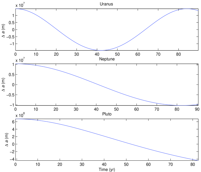
Figure 1: Semimajor axis shifts $\Delta a$, in m, for Uranus ($a=19.19$ AU), Neptune ($a=30.06$ AU) and Pluto ($a=39.48$ AU) over $T=90$ years.

The very long orbital periods of Uranus, Neptune and Pluto make also the short-period signals of interest, in principle, because they would resemble polynomial signals over observational time spans like those currently available. This could be useful especially for the semimajor axis and the eccentricity which do not exhibit secular rates. In Figure 1, Figure 2, Figure 3 and 4 we plot the total, i.e. linear (when present) and sinusoidal, integrated shifts of eqs. (12)-(14) and eq. (18) for the semimajor axis, the eccentricity, the perihelion and the mean longitude, respectively over $90$ years. In Table 3 we quote the amplitudes ${\mathcal{A}}$ of the short-period signals for Uranus, Neptune and Pluto. Anomalous signatures of such size would be detectable as well, but nothing like that is mentioned in Pitjeva’s work.

4 The orbital effects induced by a constant radial acceleration: numerical simulations and comparison with data

The Keplerian orbital elements are not directly measured quantities: they are related to data in an indirect way. For the outer planets the true observables are the right ascension $\alpha$ and the declination $\delta$. In Figure 2 of [14] there are the observational residuals of $\alpha\cos\delta$ and $\delta$ for Uranus, Neptune and Pluto from 1913 to 2004. In order to make a direct comparison with them, in this Section we numerically compute theoretical Pioneer-No Pioneer (P-NP) residuals for the same quantities over the same time span.

The first step of this process consists in a direct integration of the gravitational equations in Cartesian rectangular coordinates. A number of software packages to perform this goal are freely available on the Internet; between them there are OrbFit (http://newton.dm.unipi.it/orbfit/), ORSA (Orbit Reconstruction, Simulation and Analysis, http://orsa.sourceforge.net/, by P. Tricarico), and Mercury [18]. The last one has been chosen because it has the simplest use and allows to introduce without difficulty user-defined perturbing forces, such the Pioneer one. It is introduced through the definition of the corresponding acceleration, whose components in $x,y$ and $z$ in an heliocentric frame are given. In this implementation this acceleration has been considered only for heliocentric distances greater then 15.0 AU, so to include the whole orbit of Uranus, totally excluding Saturn. This package uses the following integration methods

• second order mixed-variable symplectic

• Bulirsh-Stoer (general)

• Bulirsh-Stoer (conservative systems)

• Radau 15th order

• hybrid (symplectic / Bulirsh-Stoer)

Since the pros and cons of a method depend to a certain extent on the specific problem to be solved, a number of tests have been performed, using most of the proposed methods and various initial conditions in order to choose the most suitable approach to our problem. performed form JD 2410000.5 to JD 2460000.5, for the nine planets As a result, the 15th order Everhart-Radau algorithm has been chosen for the Pioneer problem and initial conditions at JD 2410000.5. The output is in $XYZ$ barycentric, with both integration and tabulation steps of 10.0 days. The $XYZ$ coordinates of the Earth’s center are obtained from ORSA. The right ascensions and declinations of the three planets have been obtained in the standard way (see e.g. [19]), and the residuals in $\alpha\cos\delta$ and $\delta$ have been plotted in Figures 5-10. As already noted, Figure 2 of [14] shows the observational residuals, in ^′′, of $\alpha\cos\delta$ and $\delta$ for Jupiter, Saturn, Uranus, Neptune and Pluto; the scale is $\pm 5$ ^′′ and no secular or semi-secular trends can be recognized by visual inspection. Our numerically produced P-NP residuals of Figures 5-10 can be straightforwardly compared to the last three panels (from the bottom) of Figure 2 of [14] yielding a direct and unambiguous confrontation with the observations. As can be noted, the pattern which would be induced by a Pioneer-like acceleration on the planetary motions is absent in the data.

5 Summary and conclusions

In this paper we have considered the orbital motions of Uranus, Neptune and Pluto to investigate, from a purely phenomenological point of view, if an anomalous force field inducing a constant, uniform Sunward acceleration of $8.74\times 10^{-10}$ m s^-2, as that experienced by the Pioneer spacecraft, affects their motions which occur in the 20-40 AU region of the Solar System, well within the range in which the Pioneer data show the anomalous signature. We have worked out both analytically and numerically the perturbations induced by such a disturbing acceleration on the Keplerian orbital elements and on the directly observable right ascensions and declinations of Uranus, Neptune and Pluto. It turns out that there are long-period, secular rates on the perihelion and the mean anomaly and short-period effects on the semimajor axis, the eccentricity, the perihelion and the mean anomaly which map onto certain particular patterns of the right ascensions and declinations. Such anomalous signatures would be large enough to be detected according to the present-day accuracy in orbit determination, but there is no trace of them in the currently available data. This result restricts the possible causes of the Pioneer anomaly to some unknown forces which violate the equivalence principle in a very strange way or to some non-gravitational mechanisms peculiar to the spacecraft.

Table 1: Secular effects, in arcseconds/century (^′′ cy^-1), induced by a constant radial acceleration of magnitude $8.74\times 10^{-10}$ m s^-2 on the perihelion and mean longitude of Uranus, Neptune and Pluto.

Planet	$\varpi$	$\lambda$
Uranus	-83.5	167.401
Neptune	-104	209.48
Pluto	-116.2	241.89

Table 2: Formal standard statistical errors in the non-singular planetary orbital elements, from Table 4 of [14]. The latest EPM2004 ephemerides have been used. The realistic errors may be up to one order of magnitude larger. The units for the angular parameters are milliarcseconds (mas).

Planet	$a$ (m)	$\sin i\cos\Omega$ (mas)	$\sin i\sin\Omega$ (mas)	$e\cos\varpi$ (mas)	$e\sin\varpi$ (mas)	$\lambda$ (mas)
Mercury	0.105	1.654	1.525	0.123	0.099	0.375
Venus	0.329	0.567	0.567	0.041	0.043	0.187
Earth	0.146	-	-	0.001	0.001	-
Mars	0.657	0.003	0.004	0.001	0.001	0.003
Jupiter	639	2.410	2.207	1.280	1.170	1.109
Saturn	4222	3.237	4.085	3.858	2.975	3.474
Uranus	38484	4.072	6.143	4.896	3.361	8.818
Neptune	478532	4.214	8.600	14.066	18.687	35.163
Pluto	3463309	6.899	14.940	82.888	36.700	79.089

Table 3: Amplitudes ${\mathcal{A}}$ of the integrated short-period effects induced by a constant radial acceleration with magnitude $8.74\times 10^{-10}$ m s^-2 on the orbital elements of Uranus, Neptune and Pluto. Note that the values of ${\mathcal{A}}_{\rm\Delta\lambda}$ and the present-day errors in $\lambda$ fully justify the approximation used to work out eq. (18).

Planet	${\mathcal{A}}_{\Delta a}$ (m)	${\mathcal{A}}_{\Delta e}$	${\mathcal{A}}_{\Delta\varpi}$ (′′)	${\mathcal{A}}_{\Delta\lambda}$ (′′)
Uranus	$1.470\times 10^{7}$	$1\times 10^{-4}$	237.1	$1.848$
Neptune	$1.03\times 10^{7}$	$2.6\times 10^{-4}$	3201	$0.82$
Pluto	$6.7\times 10^{8}$	$4\times 10^{-4}$	$184.5$	$41.64$

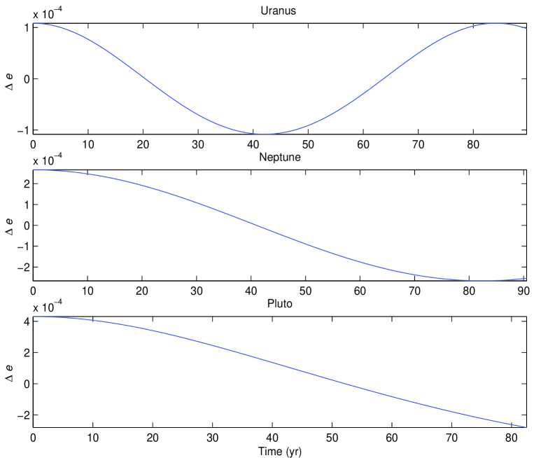
Figure 2: Eccentricity shifts $\Delta e$ for Uranus ($a=19.19$ AU), Neptune ($a=30.06$ AU) and Pluto ($a=39.48$ AU) over $T=90$ years.

Figure 3: Longitude of perihelion shifts $\Delta\varpi$, in ^′′, for Uranus ($a=19.19$ AU), Neptune ($a=30.06$ AU) and Pluto ($a=39.48$ AU) over $T=90$ years.

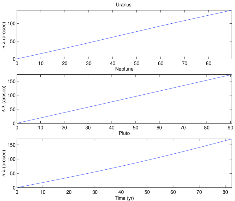
Figure 4: Mean longitude shifts $\Delta\lambda$, in ^′′, for Uranus ($a=19.19$ AU), Neptune ($a=30.06$ AU) and Pluto ($a=39.48$ AU) over $T=90$ years.

Figure 5: Numerically propagated P-NP residuals for $\alpha\cos\delta$ of Uranus from 1913 to 2004. Compare it with the third panel from the bottom of Figure 2 of [14].

Figure 6: Numerically propagated P-NP residuals for $\delta$ of Uranus from 1913 to 2004. Compare it with the third panel from the bottom of Figure 2 of [14].

Figure 7: Numerically propagated P-NP residuals for $\alpha\cos\delta$ of Neptune from 1913 to 2004. Compare it with the second panel from the bottom of Figure 2 of [14].

Figure 8: Numerically propagated P-NP residuals for $\delta$ of Neptune from 1913 to 2004. Compare it with the second panel from the bottom of Figure 2 of [14].

Figure 9: Numerically propagated P-NP residuals for $\alpha\cos\delta$ of Pluto from 1913 to 2004. Compare it with the first panel from the bottom of Figure 2 of [14].

Figure 10: Numerically propagated P-NP residuals for $\delta$ of Pluto from 1913 to 2004. Compare it with the first panel from the bottom of Figure 2 of [14].

References

- [1]
- [2] Toth, V., and Turyshev, S.G., The Pioneer Anomaly: Seeking an explanation in newly recovered data, gr-qc/0603016, 2006.
- [3] Anderson, J.D.,Laing, P.A., Lau, E.L., Liu, A.S., Nieto, M.M., and Turyshev, S.G., Indication, from Pioneer 10/11, Galileo, and Ulysses Data, of an Apparent Anomalous, Weak, Long-Range Acceleration, Phys. Rev. Lett., 81, 2858-2861, 1998.
- [4] Anderson, J.D.,Laing, P.A., Lau, E.L., Liu, A.S., Nieto, M.M., and Turyshev, S.G., Study of the anomalous acceleration of Pioneer 10 and 11, Phys. Rev. D, 65, 082004, 2002.
- [5] Turyshev, S.G., Toth, V.T., Kellogg, L.R., Lau, E.L., and Lee, K.J., The Study of the Pioneer Anomaly: New Data and Objectives for New Investigation, gr-qc/0512121, 2005.
- [6] Katz, J.I., Comment on Indication, from Pioneer 10/11, Galileo, and Ulysses Data, of an Apparent Anomalous, Weak, Long-Range Acceleration , Phys. Rev. Lett., 83, 1892, 1999.
- [7] Nieto, M.M., and Turyshev, S.G., Finding the Origin of the Pioneer Anomaly, Class. Quantum Grav., 21, 4005-4024, 2004.
- [8] Penanen, K., and Chui, T., A Novel Two-Step Laser Ranging Technique for a Precision Test of the Theory of Gravity, Nucl. Phys. Suppl. Proc., 134, 211-213, 2004.
- [9] Izzo, D., and Rathke, A., Options for a non-dedicated test of the Pioneer anomaly, astro-ph/0504634, 2005.
- [10] Dittus, H., Turyshev, S.G., Lämmerzahl, C., Theil, S., Förstner, R., Johann, U., Ertmer, W., Rasel, E., Dachwald, B. Seboldt, W., Hehl, F.W., Kiefer, C., Blome, H.-J., Kunz, J., Giulini, D., Bingham, R., Kent, B., Summer, T.J., Bertolami, O., Páramos, J., Rosales, J.L., Cristophe, B., Foulon, B., Touboul, P., Bouyer, P., Reynaud, S., Brillet, A., Bondu, F., Samain, E., de Matos, C.J., Erd, C., Grenouilleau, J.C., Izzo, D., Rathke, A., Anderson, J.D., Asmar, S.W., Lau, E.E., Nieto, M.M., and Mashhoon, B., A mission to explore the Pioneer anomaly, invited talk given at the 2005 ESLAB Symposium Trends in Space Science and Cosmic Vision 2020, 19-21 April 2005, ESTEC, Noordwijk, The Netherlands, gr-qc/0506139, 2005.
- [11] Page, G., Dixon, D.S., and Wallin, J.F., Can Minor Planets be Used to Assess Gravity in the Outer Solar System?, astro-ph/0504367, 2005; American Astronomical Society Meeting 207, 154.02, 2005.
- [12] Tangen, K., Could the Pioneer anomaly have a gravitational origin? gr-qc/0602089, 2006.
- [13] Standish, E.M., An approximation to the errors in the planetary ephemerides of the Astronomical Almanac, Astron. Astrophys., 417, 1165-1171, 2004.
- [14] Pitjeva, E.V., High-Precision Ephemerides of Planets-EPM and Determination of Some Astronomical Constants, Sol. Sys. Res., 39, 176-186, 2005.
- [15] Milani, A., Nobili, A.M, and Farinella, P., Non-gravitational perturbations and satellite geodesy, (Adam Hilger, Bristol, 1987).
- [16] Boltz, F.W., Orbital Motion Under Continuous Radial Thrust, J. of Guidance, Control, and Dynamics, 14, 667-670, 1991.
- [17] Prussing, J.E., and Coverstone-Carroll, V., Constant Radial Thrust Acceleration Redux, J. of Guidance, Control, and Dynamics, 21, 516-518, 1998.
- [18] Chambers, J.E., A hybrid symplectic integrator that permits close encounters between massive bodies, Mon. Not. Roy. Astron. Soc., 304, 793-799, 1999.
- [19] Meeus, J., Astronomical Algorithms, (Willman-Bell, 1999).