New, efficient, and accurate high order derivative and dissipation operators satisfying summation by parts, and applications in three-dimensional multi-block evolutions

Abstract

We construct new, efficient, and accurate high-order finite differencing operators which satisfy summation by parts. Since these operators are not uniquely defined, we consider several optimization criteria: minimizing the bandwidth, the truncation error on the boundary points, the spectral radius, or a combination of these. We examine in detail a set of operators that are up to tenth order accurate in the interior, and we surprisingly find that a combination of these optimizations can improve the operators’ spectral radius and accuracy by orders of magnitude in certain cases. We also construct high-order dissipation operators that are compatible with these new finite difference operators and which are semi-definite with respect to the appropriate summation by parts scalar product. We test the stability and accuracy of these new difference and dissipation operators by evolving a three-dimensional scalar wave equation on a spherical domain consisting of seven blocks, each discretized with a structured grid, and connected through penalty boundary conditions.

I Introduction

Kreiss and Scherer proposed quite some time ago Kreiss and Scherer (1974, 1977) a powerful way of constructing linearly stable schemes for solving evolution partial differential equations which admit an energy estimate at the continuum, through the use of difference operators satisfying summation by parts (SBP). These operators essentially make it possible, up to boundary terms, to derive estimates analogous to the continuum ones. While the latter guarantee well posedness, their discrete counterparts guarantee numerical stability. The boundary terms left after SBP can be controlled by, for example, orthogonal projections Olsson (1995a, b, c), penalty terms Carpenter et al. (1994), or a combination of them Gustafsson (1998) (see Mattsson (2003); Strand (1996) for a comparison between these methods). Furthermore, SBP difference operators and penalty techniques have been rather recently combined to construct stable schemes of arbitrary high order for multi-block simulations Carpenter et al. (1999); Nordström and Carpenter (2001). These are simulations where the domain is broken into different sub-domains which are “glued” together through an appropriate interface treatment, in this case penalty terms. This semi-structured approach allows for non-trivial geometries while at the same time ensuring stability for schemes of arbitrary high order using derivatives satisfying SBP.

Systems which have smooth solutions (that is, without shocks), such as the Einstein vacuum equations (see, for example, Reula (1998)), are ideal for using high order methods. Furthermore, in numerical relativity one typically deals with non-trivial topologies and the need for smooth boundaries. Although there are proofs for particular systems in non-smooth domains, proofs of well posedness for the initial-boundary value problem for general symmetric hyperbolic systems usually require smooth outer boundaries Rauch (1985); Secchi (1996a, b).

Multi-block domains are also more efficient than single-block ones, as they can be chosen to adapt to particular situations. For instance, they can be made to mimic spherical coordinates which automatically reduce the angular resolution at large radii (this allowed, for example, studying late time behavior in a rotating black hole background in full three-dimensions, placing the outer boundary at very large distances with modest computational resources Lehner et al. (2005)), and one can also reduce the radial resolution (e.g. logarithmically). Last, the need for non-trivial topologies includes the particular but very important case of black hole excision, where the black hole singularity is removed from the computational domain. In sum, the penalty multi-block approach combined with high order SBP operators appears to be promising for simulating Einstein’s equations.

In principle, modulo the tedious but straightforward symbolic manipulation algebra needed to construct high order difference operators satisfying SBP, one can systematically generate in this way stable multi-block schemes of arbitrary high order. However, it turns out that high order operators satisfying SBP are highly non-unique, the higher their order the higher their non-uniqueness. There is great variation among the properties of these operators, and for reasons that we discuss below, much care has to be taken in choosing the stencils if explicit time integration schemes are used. One approach could involve choosing operators with minimum bandwidth, as they reduce the number of operations. Unfortunately, in some cases the resulting operator leads to an amplification matrix with a very large spectral radius (which has already been pointed out in Lehner et al. (2005) and Svärd et al. (2005)); when using explicit schemes to integrate in time, this translates into a very small Courant limit. One can do much better by attempting to minimize the spectral radius of the complete operator, rather than its bandwidth. This in some cases leads to a Courant limit two orders of magnitude larger as compared to the minimum bandwidth case. One can sometimes do even better: another feature to take into account is the amplitude of the truncation errors at and close to boundaries. As we will show, in some cases one can decrease them by orders of magnitude while keeping the spectral radius small. What we have just briefly discussed is one of the goals of this paper, namely to explicitly construct efficient and accurate high order SBP difference operators, and compare the above different criteria that can be used in their construction. We consider both diagonal and restricted full (non-diagonal) norm based operators; in the first (second) case up to order ten (eight) in the interior.

In many cases of interest, particularly in non-linear ones, one might want to add a small amount of artificial dissipation to the problem. In order not to spoil the available energy estimates, the dissipation operator has to be negative semi-definite with respect to the SBP scalar product. This is not just a technical detail. As we will discuss below, in certain cases of interest the use of simple dissipation operators that do not satisfy this property (e.g. standard Kreiss–Oliger dissipation in the interior and no dissipation near boundaries, a choice commonly used in some applications) cannot get rid of some instabilities, while better dissipation operators do. Even if there are no instabilities, a dissipation operator that is non-zero close to boundaries is very useful if one wants to smooth out aspects of the solution propagating through the multi-block interfaces. Mattsson et al. Mattsson et al. (2004) have recently presented a way of constructing dissipation operators that are indeed negative semi-definite for arbitrary SBP scalar products, and which extend all the way up to the boundaries. Following this prescription one can construct, for any difference operator of arbitrary high order satisfying SBP, an associated dissipation up to the very boundary points in a systematic way. In this paper we do so explicitly, for each of the efficient and accurate high order derivatives that we present. This is the second goal of our paper.

The third and final goal is to test these new derivative and dissipation operators in three-dimensional multi-block simulations, making use of the penalty method to handle interfaces, as described in Carpenter et al. (1999); Nordström and Carpenter (2001). Because of the challenge involved in achieving stability for very high order schemes in the presence of interfaces, multi-block domains present an ideal setting for testing the new derivative and dissipation operators that we here construct. While black hole excision is one of our main motivations for using multiple blocks, we will report here on simulations on a domain that is useful for scenarios that do not involve black hole excision, but still need a smooth (e.g. spherical) outer boundary. This grid structure should be useful for studies of wave phenomena at large distances from the source, gravitational collapse, or Friedrich’s conformal approach, where the spacetime is compactified, and null infinity is brought to a finite computational distance (see e.g. Friedrich (2002)). In order to isolate testing numerical stability, accuracy, and efficiency of the new high order derivative and dissipation operators from gauge problems and continuum instabilities typically found in many formulations of the Einstein equations, we perform these tests in this paper using a simpler three-dimensional system —a massless scalar field— and we will report on evolutions of the Einstein equations elsewhere.

This paper is organized as follows. In Section II we introduce our notation, review shortly the penalty method, discuss the relative merits of SBP finite differencing operators based on diagonal and on non-diagonal norms, and summarize the construction of dissipation operators of Mattsson et al. Mattsson et al. (2004). In Section III, we explain the different strategies that we use in constructing the new derivative operators, namely their bandwidth, their spectral radius, and their truncation error. We introduce our example system of evolution equations in Section IV, where we also describe the type of three-dimensional multi-block domain that we use to test the new difference and dissipation operators. We describe our new operators corresponding to diagonal and restricted full norms in Section V, discussing their properties and comparing their accuracies in numerical tests. Finally, Section VI closes with some remarks about possible future research directions.

II SBP derivative and dissipation operators with a high order of accuracy

II.1 SBP and penalties

In this subsection we briefly summarize Section 2 of Lehner et al. (2005). We do so essentially to fix our notation, for more details see that reference. Consider a computational domain $[a,b]$ and a discrete grid consisting of points $i=1\ldots n$ and grid spacing $h$. A difference operator $D$ is said to satisfy SBP on that domain with respect to a positive definite scalar product $\Sigma$ (defined by its coefficients $\sigma_{ij}$)

$$\langle u,v\rangle=h\sum_{i,j=1}^{n}u_{i}v_{j}\sigma_{ij}\,,$$ (1)

if the property

$$\langle u,Dv\rangle+\langle v,Du\rangle=\left(uv\right)|_{a}^{b}$$ (2)

holds for all grid functions $u$ and $v$. Similar definitions can be introduced for two (and higher) dimensional domains. The scalar product or norm is said to be diagonal if

$$\sigma_{ij}=\sigma_{ii}\delta_{ij}\;\textrm{,}$$ (3)

that is, if $\sigma_{ij}$ is diagonal. It is called restricted full if

$$\sigma_{i_{b}j}=\sigma_{i_{b}i_{b}}\delta_{i_{b}j}\;\textrm{,}$$ (4)

that is, if $\sigma_{ij}$ is diagonal on the boundary, but may be non-diagonal (full) in the interior. $i_{b}\in\{1,n\}$ denote boundary point indices.

We now briefly highlight through a simple example the main features of the penalty method for multi-block evolutions, for more details see Carpenter et al. (1999); Nordström and Carpenter (2001). We assume that the norm is either diagonal or restricted full, since these are the cases we actually consider later in this paper.

The simple example we wish to consider is the advection equation,

$$\partial_{t}u=\Lambda\partial_{x}u$$

in the spatial interval $(-\infty,+\infty)$ with appropriate fall-off conditions at infinity, and two grids: a left grid covering $(-\infty,0]$, and a right grid covering $[0,+\infty)$. We refer to the grid function $u$ on each grid by $u^{l}$ and $u^{r}$, corresponding to the left and right grids, respectively. The problem is discretized using grid spacings $h^{l},h^{r}$ on the left and right grids —not necessarily equal— and difference operators $D^{l},D^{r}$ satisfying SBP with respect to scalar products given by the weights $\sigma^{l},\sigma^{r}$ on their individual grids. That is, these scalar products are defined through

$$\langle u^{l},v^{l}\rangle=h^{l}\sum_{i,j=-\infty}^{0}\sigma^{l}_{ij}u^{l}_{i}v^{l}_{j}\;\;\;,\;\;\;\langle u^{r},v^{r}\rangle=h^{r}\sum_{i,j=0}^{+\infty}\sigma^{r}_{ij}u^{r}_{i}v^{r}_{j}$$ (5)

The semi-discrete equations are written as

$$\partial_{t}u^{l}_{i} = \Lambda D^{l}u^{l}_{i}+\frac{\delta_{i,0}S^{l}}{h^{l}\sigma^{l}_{00}}(u^{r}_{0}-u^{l}_{0})\;\textrm{,}$$ (6)

$$\partial_{t}u^{r}_{i} = \Lambda D^{r}u^{r}_{i}+\frac{\delta_{i,0}S^{r}}{h^{r}\sigma^{r}_{00}}(u^{l}_{0}-u^{r}_{0})\;\textrm{.}$$ (7)

In the fully non-diagonal case the treatment is slightly more complicated, therefore we consider here only the diagonal and the restricted full cases.

One can derive an energy estimate and therefore guarantee stability if two conditions are satisfied. One of them is $\Lambda+S_{r}-S_{l}=0$. The other one imposes an additional constraint on the values of $S_{l}$ and $S_{r}$:

• Positive $\Lambda$:

  $$S_{l}=\Lambda+\delta,\;\;\;S_{r}=\delta,\;\;\;\mbox{ with }\delta\geq-\frac{\Lambda}{2}$$ (8)

• Negative $\Lambda$:

  $$S_{r}=-\Lambda+\delta,\;\;\;S_{l}=\delta,\;\;\;\mbox{ with }\delta\geq\frac{\Lambda}{2}$$ (9)

• Vanishing $\Lambda$: this can be seen as the limiting case of any of the above two.

For the minimum values of $\delta$ allowed by the above inequalities the energy estimate is the same as for a single grid (that is, as if the interface did not exist), while for larger values of $\delta$ there is damping in the energy which is proportional to the mismatch at the interface.

II.2 Diagonal versus non-diagonal norms

There are several advantages in using one-dimensional (1D) difference operators satisfying SBP with respect to diagonal norms. One of them is related to the fact that SBP is guaranteed to hold in several dimensions by simply applying the 1D operator along each direction Olsson (1995a, b, c). Another advantage is related to the following: in order to ensure stability through an energy estimate, in many cases one has to be able to bound the norm of the commutator between the difference operator and the principal part of the equations for all resolutions, and this is guaranteed to hold in the diagonal case. Finally, the expressions of the operators are also somewhat simpler when compared to non-diagonal ones. The disadvantage, on the other hand, is that the order of accuracy at and close to boundaries is half of that in the interior, while in the restricted full case the operators lose only one order near boundaries Kreiss and Scherer (1974, 1977); Strand (1994).

Though more efficient, schemes based on non-diagonal norms might have stability problems in the absence of dissipation. First, it is not guaranteed that SBP holds in several dimensions if a difference operator satisfying SBP in 1D is applied along each direction. Second, there can be problems even in one dimension when the system has variable coefficients, since the boundedness of the commutator discussed above is not guaranteed to hold either. This is not a feature inherent to finite difference (FD)-based schemes: the boundedness of such commutator is, for example, in general not guaranteed either for pseudo-spectral methods in the absence of filtering, even in periodic domains, when the system has variable coefficients Tadmor (1994). Therefore, both in the case of pseudo-spectral methods and non-diagonal norm based FD schemes, one is in general unable to guarantee stability in more than one dimension, or even in 1D in the variable coefficient case, without filtering or dissipation (see also Svärd (2005)). In the problem at hand, the question then is whether one can stabilize the scheme through artificial dissipation, without introducing an excessive amount of it. Below we will address this question in detail, as well as compare diagonal based operators to their non-diagonal counterparts.

In the diagonal case we will consider difference operators of order two, four, six, eight, and ten in the interior (and therefore order one, two, three, four and five, respectively, at and close to boundaries) and denote them by $D_{2-1},D_{4-2},D_{6-3},D_{8-4},D_{10-5}$. In the non-diagonal (restricted full) case, we will consider operators of order four, six and eight in the interior (and therefore order three, five and seven, respectively, at and close to boundaries), and denote them by $D_{4-3},D_{6-5},D_{8-7}$. These operators in general are not unique. For example, in the second order in the interior case there is a unique operator satisfying SBP, and its norm is diagonal, the operator being what we called $D_{2-1}$. With respect to higher order operators, the following holds for the diagonal norm based ones: $D_{4-2}$ is unique, while $D_{6-3}$, $D_{8-4}$ and $D_{10-5}$ comprise a one-, three-, and ten-parameter family, respectively. In the restricted full case, $D_{4-3}$, $D_{6-5}$ and $D_{8-7}$ have three, four and five free parameters, respectively.

II.3 Dissipation operators

As pointed out in Mattsson et al. (2004), adding artificial dissipation may lead to an unstable scheme unless the dissipation operator is compatible with the SBP derivative operator. In that reference, the authors present a prescription for constructing such operators, which we follow here. In short, a compatible dissipation operator, of order $2p$ in the interior, is constructed as

$$A_{2p}=-\alpha\,h^{2p}\;\Sigma^{-1}D_{p}^{T}B_{p}D_{p},$$ (10)

where $\alpha$ is a positive constant, $\Sigma$ is the scalar product used in the construction of the SBP operator, and $D_{p}$ is a consistent approximation of $d^{p}/dx^{p}$ with minimal width. $B_{p}$ is the so-called boundary operator. The boundary operator is positive semi-definite and its role is to allow boundary points to be treated differently from interior points. $B_{p}$ cannot be chosen freely, but has to follow certain restrictions which we explain below.

For the diagonal norm operators, choosing $B_{p}$ to be the unit matrix is sufficient to obtain the required $p$th order accuracy near the boundary, which is the same accuracy as the derivative operator.

In the case of restricted full norm operators, the accuracy requirement near the boundary is stricter. The dissipation operator should have order $2p-1$ at the boundary and order $2p$ in the interior, which requires a different choice of $B_{p}$. We again follow Mattsson et al. (2004) and choose $B_{p}$ to be a diagonal matrix, where the diagonal is the restriction onto the grid of a piecewise smooth function. The numerical domain is divided into three regions in each dimension; an interior part and on either side two transition regions containing the boundaries. The transition region has a fixed size that is independent of the resolution. Within the transition region the function, $B_{p}$, increases from $O(h^{p-1})$ at the outer boundary to a constant value $1$ at the boundary with the interior region in such a way that the derivatives of $B_{p}$ up to order $p-2$ vanish at either ends. In the interior region the function has the constant value $1$.

For the $D_{4-3}$ operator, $B_{p}$ has the value $h$ at the boundary and increases linearly to $1$ in the transition region. For the $D_{6-5}$ operator, we use a cubic polynomial with vanishing derivatives at either end of the transition region to increase the value of $B_{p}$ from $h^{2}$ at the boundary to $1$ in the interior. For the $D_{8-7}$ operator, the boundary values for the transition region are $h^{3}$ and $1$, and we use a fifth order polynomial to make the first and second derivatives vanish at either end of the transition region.

For the constant $\alpha$ we make the choice $\alpha=2^{-2p}$, since then the parameter used to specify the strength of the dissipation has approximately the same allowed numerical range, independently of the order of the operator.

Note that in the diagonal case up to order eight in the interior, the scalar product $\Sigma$ is independent of the free parameters, so for a given order the same dissipation operator is used for all the different operators we construct below, while for the higher order diagonal operators and the restricted full norm operators a unique dissipation operator has to be constructed for each parameter choice.

III Optimization criteria

We start by fixing some notation. If the accuracy of the difference operator $D$ in the interior is $2p$, then there are $b$ points at and near the boundaries where the order of $D$ is only $q$. In the diagonal case one has $q=p$, and in the restricted full case it is $q=2p-1$. We call $b$ the boundary width. The difference operator at these $b$ points uses (up to) $s$ points to compute the derivative. We call $s$ the boundary stencil size.

When expanding $D$ in a Taylor series one has

$$\left.Du\right|_{x_{i}}=\left.\frac{du}{dx}\right|_{x_{i}}+c_{i}h^{q}\left.\frac{d^{q+1}u}{dx^{q+1}}\right|_{x_{i}}\quad\mathrm{for}\;i=1\ldots b$$ (11)

where $h$ is the grid spacing and $x_{i}=ih$. We call $c_{i}$ the error coefficients.

In what follows, we consider three cases for each family of operators of a given order, denoted by:

• Minimum bandwidth: If there are $n$ free parameters, it is always possible to set $n$ of the derivative coefficients to zero, thereby minimizing the computational cost of evaluating the derivatives in the boundary region.

• Minimum spectral radius: In this case, we calculate numerically the eigenvalues of the amplification matrix for a test problem, and choose the parameters to minimize the largest eigenvalue.

• Minimum ABTE: We minimize the average boundary truncation error (ABTE), which we define as

  $$\textrm{ABTE}:=\left(\frac{1}{b}\sum_{i=1}^{b}c_{i}^{2}\right)^{1/2}.$$ (12)

The test problem that we use to compute the spectral radius of the amplification matrix is the same one that was used in Lehner et al. (2005): an advection equation propagating in a periodic domain. Periodicity is enforced through an artificial interface boundary via penalties. We use a penalty parameter $\delta=-1/2$ (see Section II), which means that the semi-discrete energy is strictly preserved, and that the amplification matrix is anti-Hermitian, and therefore the real part of all eigenvalues is zero.

Another option Svärd et al. (2005) would be to compute the spectral radius of the discrete difference operator itself. In this case, the spectrum is in general not purely imaginary, since the boundary conditions have not been imposed yet. In practice we have found, though, that both approaches lead to similar operators, in the sense that a derivative operator with small spectral radius usually also leads to amplification matrices for the above test problem with small spectral radii as well.

It is worth pointing out that for the diagonal operator case the bandwidth and the ABTE can be globally minimized by analytically choosing the parameters, since the ABTE is a quadratic function of the parameters and therefore has a global minimum. This is not the case for the spectral radius. Therefore, when we refer to minimizing the spectral radius, we perform a numerical minimization and do not claim that we have actually found a global minimum.

IV Example evolution system and multi-block domain setup

We test each of the new derivative operators and their associated dissipation operators through 3D multi-block simulations. In these simulations we solve the scalar wave equation

$$\partial_{tt}\phi=\Delta\phi$$ (13)

in static, curvilinear coordinates. This equation can be reformulated as

$$\partial_{t}\phi = \Pi$$ (14)

$$\partial_{t}\Pi = \gamma^{-1/2}D_{i}\left(\gamma^{1/2}\gamma^{ij}d_{j}\right)$$ (15)

$$\partial_{t}d_{i} = D_{i}\Pi\;,$$ (16)

where $\gamma_{ij}$ is the Euclidean metric in curvilinear coordinates, $\gamma=\det\gamma_{ij}$ its determinant, and $\gamma^{ij}$ its inverse. Here we use the Einstein summation convention, implicitly summing over repeated indices.

The advantage of this particular form of the equations is that it defines a strictly stable discretization in the diagonal case, in the sense that one can show by just using SBP (i.e., without needing a discrete Leibniz rule, which in general does not hold) that there is a semi-discrete energy $E$ which is preserved in time for any difference operator $D$ satisfying SBP. This energy is given by

$$E=\frac{1}{2}\int\left(\Pi^{2}+\gamma^{ij}d_{i}d_{j}\right)\,\gamma^{1/2}\;dV.$$ (17)

The geometry of the computational domain in the three-dimensional (3D) simulations that we show below is the interior of a sphere. In order to avoid the singularities at the origin and poles that spherical coordinates have, we cover the domain with seven blocks: surrounding the origin we use a Cartesian, cubic block, which is matched (at each face) to a set of six blocks which are a deformation of the cubed-sphere coordinates used in Lehner et al. (2005). Figure 1 shows an equatorial cut of our 3D grid structure, for $11^{3}$ points on each block. The blocks touch and have one grid point in common at the faces. The grid lines are continuous across interfaces, but in general not smooth.

Each block uses coordinates $a,b,c$. For the inner block these are the standard Cartesian ones: $a=x,b=y,c=z$, while for the six outer blocks they are defined as follows. The “radial” coordinate $c\in[-1,1]$ is defined by inverting the relationship

$$r=\frac{1}{2}\left[r_{0}(1-c)+r_{1}(1+c)\right]$$ (18)

(where $r=\sqrt{x^{2}+y^{2}+z^{2}}$). The “angular” coordinates, $a,b\in[-1,1]$, are in turn defined through

• Neighborhood of positive $x$ axis:
  $x=r/F,\quad y=rb/F,\quad z=ar/F$

• Neighborhood of positive $y$ axis:
  $x=-br/F,\quad y=r/F,\quad z=ar/F$

• Neighborhood of negative $x$ axis:
  $x=-r/F,\quad y=-rb/F,\quad z=ar/F$

• Neighborhood of negative $y$ axis:
  $x=br/F,\quad y=-r/F,\quad z=ar/F$

• Neighborhood of positive $z$ axis:
  $x=-ar/F,\quad y=rb/F,\quad z=r/F$

• Neighborhood of negative $z$ axis:
  $x=ar/F,\quad y=rb/F,\quad z=-r/F$

where $r$ is written in terms of $c$ through (18), and

$$F := \left(\frac{(r_{1}-r)+(r-r_{0})E}{r_{1}-r_{0}}\right)^{1/2}$$ (19)

with $E=1+a^{2}+b^{2}$. The surface $c=1$ corresponds to the spherical outer boundary (of radius $r=r_{1}$), while $c=-1$ corresponds to the cubic interface boundary matched to a cube of length $2r_{0}$ on each direction. The grid structure of Figure 1 corresponds to $r_{0}=1$, $r_{1}=3$.

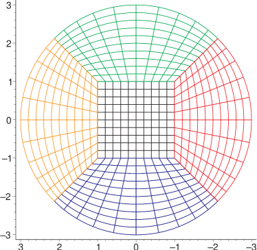
Figure 1: An equatorial cut of the 3D multi-block structure used in the simulations of this paper.

To get an accurate measure of numerical errors, we evolve initial data for which there exists a simple analytic solution of (14) for all times, against which we can compare the numerical results. We choose initial data

$$\phi(t=0) = A\cos(2\pi\bm{k}\cdot\bm{x})$$ (20)

$$\Pi(t=0) = -2\pi A|\bm{k}|\sin(2\pi\bm{k}\cdot\bm{x})$$ (21)

$$d_{i}(t=0) = -2\pi Ak_{i}\sin(2\pi\bm{k}\cdot\bm{x}).$$ (22)

The analytic solution for this setup is a plane wave with constant amplitude $A$ traveling through the grid in the direction of the vector $\bm{k}$. In all the simulations that we present below we use $A=1.0$ and $\bm{k}=(0.2,0.2,0.2)$, i.e., the wave is traveling in the direction of the main diagonal. Consistent and stable outer boundary conditions are imposed through penalty terms by penalizing the incoming characteristic modes with the difference to the exact solution, as introduced in Carpenter et al. (1994). As mentioned above, we set $r_{0}=1$ and $r_{1}=3$ in our block system, placing the outer boundary at $R=3$.

We use resolutions from $h=\Delta a=\Delta b=\Delta c=0.1$ ($21^{3}$ grid points per block) up to $h=0.0125$ ($161^{3}$ grid points per block). Our highest resolution corresponds to about $400$ grid points per wave length. (This figure depends on which part of which block one looks at, since the wave does not propagate everywhere along grid lines.) We use that many grid points per wave length —or, equivalently put, we use such a large wave length— because we are interested in high accuracy. Decreasing the wave length is resolution-wise equivalent to using fewer grid points per block, which is a case we study with our coarse resolution. It would be interesting to study the effect of very short length features onto the stability of the system, i.e., to use a wave length that cannot be well resolved any more. Discrete stability guarantees in this case that the evolution remains stable, and we assume that a suitable amount of artificial dissipation can help in the non-linear case when there is no known energy estimate. The size of the time step is chosen to be proportional to the minimal grid spacing in local coordinates $\Delta t=\lambda\,\min(\Delta a,\Delta b,\Delta c)$ with the Courant factor $\lambda$. Unless otherwise stated, we use $\lambda=0.25$. For the penalty terms, we used $\delta=0$ everywhere. For all the runs with dissipation the strength was chosen to be $\epsilon=0.4$ (see Appendix A.2). For the dissipation operators based on a non-diagonal norm, we choose the transition region to be $30$% of the domain size. Note that except for the $D_{6-5}$ operator (where dissipation is essential in order to stabilize the operator) the differences between results with and without dissipation are so small, that we only show the results obtained without dissipation. In all cases we calculate the error in the numerical solution for $\phi(\bm{x},t)$ with respect to the exact analytical solution.

We have implemented our code in the Cactus framework Goodale et al. (2003); cac using the Carpet infrastructure Schnetter et al. (2004); car .

V Operators

V.1 Operators based on diagonal norms

V.1.1 Operator properties

We consider first operators that are based on a diagonal norm, since this is the easier case. We examine here the operators $D_{6-3}$, $D_{8-4}$, and $D_{10-5}$. These operators have 6, 8, and 11 boundary points, respectively, and their maximum stencil sizes are 9, 12, and 16 points, respectively. The operators $D_{2-1}$ and $D_{4-2}$ are also based on a diagonal norm. They are unique and have been examined in Lehner et al. (2005). For completeness we list their properties here as well.

The $D_{2-1}$ operator formally has two boundary points and a maximal stencil size of three points. However, the stencil for the second boundary point is the same as the interior centered stencil, so in practice it has only one boundary point with a stencil size of two points. The spectral radius and error coefficient are listed in table 1.

Table 1: Properties of the $D_{2-1}$ operator.

Operator	Unique
Spectral radius	$1.414$
ABTE	$0.25$
$c_{1}$	$0.5$

The $D_{4-2}$ operator has four boundary points and a maximal stencil size of six points. We list its properties in table 2.

Table 2: Properties of the $D_{4-2}$ operator.

Operator	Unique
Spectral radius	$1.936$
ABTE	$0.2276$
$c_{1}$	$-0.4215$
$c_{2}$	$0.1666$
$c_{3}$	$-0.0193$
$c_{4}$	$-0.037$

The family of $D_{6-3}$ operators has one free parameter. The resulting norm is positive definite, and is independent of this parameter, hence the parameter can be freely chosen. For this operator there are very small numerical differences in the spectral radius and in the truncation error coefficients between the three different cases where the bandwidth, the spectral radius and the average boundary truncation error are respectively minimized, as can be seen in table 3.

Table 3: Properties of the diagonal norm $D_{6-3}$ operators.

	Minimum	Minimum	Minimum
Operator	bandwidth	spectral radius	ABTE
Spectral radius	$2.1287$	$2.1077$	$2.1082$
ABTE	$0.2716$	$0.2563$	$0.2558$
$c_{1}$	$0.5008$	$0.5436$	$0.5374$
$c_{2}$	$-0.1854$	$-0.2340$	$-0.2270$
$c_{3}$	$-0.2144$	$0.0012$	$-0.0300$
$c_{4}$	$0.3067$	$0.1977$	$0.2135$
$c_{5}$	$-0.1288$	$-0.0546$	$-0.0654$
$c_{6}$	$-0.0286$	$-0.0419$	$-0.0400$

Based on those small differences one would expect that there should not be much of a difference in terms of accuracy among these three different cases in practical simulations. However, it turns out that the minimum bandwidth operator in practice leads to very different solution errors compared to the minimum ABTE operator, and that the latter is to be preferred. We did not implement the minimum spectral radius operator, since the difference in spectral radius is minimal.

The family of $D_{8-4}$ operators has three free parameters; as in the previous case, the norm is positive definite and independent of the parameters, which can therefore be freely chosen. We again investigate the properties of the operators obtained by minimizing the bandwidth, the spectral radius, and the ABTE. Interestingly, we find out that there is a one parameter family of operators that minimizes the ABTE. Therefore, in the minimum ABTE case we make use of this freedom and also decrease the spectral radius as much as possible. The results are shown in table 4.

Table 4: Properties of the diagonal norm $D_{8-4}$ operators.

	Minimum	Minimum	Minimum
Operator	bandwidth	spectral radius	ABTE
Spectral radius	$16.0376$	$2.229$	$2.231$
ABTE	$1.2241$	$0.3993$	$0.3474$
$c_{1}$	$-0.5878$	$-0.8277$	$-0.8086$
$c_{2}$	$0.1068$	$0.3682$	$0.3439$
$c_{3}$	$3.1427$	$-0.3819$	$0.0228$
$c_{4}$	$-0.7918$	$-0.2186$	$-0.3086$
$c_{5}$	$0.9886$	$-0.3412$	$0.0225$
$c_{6}$	$0.3304$	$0.3619$	$0.2970$
$c_{7}$	$-0.1995$	$-0.1097$	$-0.0823$
$c_{8}$	$-0.0211$	$-0.0465$	$-0.0497$

In this case, the minimum bandwidth operator is quite unacceptable due to its large spectral radius. (For this reason we did not even implement it.) The error coefficients are also quite large compared to the two other cases. The differences in error coefficients between the minimum spectral radius operator and the minimum ABTE operator might appear quite small, but as demonstrated in figure 5 below, there is almost of factor of two in the magnitude of the error in our numerical tests (see below).

The family of $D_{10-5}$ operators turns out to be different from the lower order cases. The conditions the SBP property impose on the norm do not yield a positive definite solution with a boundary width of 10 points. When using a boundary width of 11 points instead, there is a free parameter in the norm, which for a very narrow range of values does allow it to be positive definite. We choose this parameter to be approximately in the center of the allowed range. With the larger boundary width, there are 10 free parameters in the difference operator. Fixing these to give a minimal bandwidth operator results in an operator with a large ABTE (20.534) and very large spectral radius (995.9) that is not of practical use. Minimizing the spectral radius in the full 10 dimensional parameter space turned out to be very difficult because the largest imaginary eigenvalue does not vary smoothly with the parameters. Instead we attempted to minimize the average magnitude of all the eigenvalues, however the resulting operator turned out to have a slightly larger spectral radius than the minimum ABTE operator considered next and were therefore not implemented and tested. Minimizing the ABTE instead fixes four of the ten parameters and the remaining six can then be used to minimize the spectral radius. This results in an operator with a ABTE of 0.7661 and spectral radius of 2.240. When used in practice, it turns out that this operator at moderate resolutions has rather large errors compared to the corresponding $D_{8-4}$ case. The errors can be reduced by a factor of about 3 by adding artificial dissipation, indicating that the errors, though not growing in time, are dominated by high frequency noise from the boundary derivative operators. Only at the highest resolution considered in the tests of this paper is there an advantage in using the $D_{10-5}$ operators. We therefore do not pursue them further in this paper, though we might consider their use in other applications if we need higher resolutions.

For completeness we list the properties of the minimum bandwidth and ABTE $D_{10-5}$ operators in table 5.

Table 5: Properties of the diagonal norm $D_{10-5}$ operators.

	Minimum	Minimum
Operator	bandwidth	ABTE
Spectral radius	$995.9$	$2.240$
ABTE	$20.534$	$0.7661$
$c_{1}$	$0.7270$	$2.0379$
$c_{2}$	$0.3034$	$-0.8545$
$c_{3}$	$-10.5442$	$-0.0898$
$c_{4}$	$0.2690$	$0.7250$
$c_{5}$	$4.8373$	$0.2889$
$c_{6}$	$-62.3907$	$-0.0154$
$c_{7}$	$-1.3649$	$-0.6429$
$c_{8}$	$24.6628$	$0.0293$
$c_{9}$	$0.1045$	$0.7073$
$c_{10}$	$-0.4197$	$-0.1411$
$c_{11}$	$-0.0243$	$-0.1469$

V.1.2 Numerical tests

In the diagonal case we do not need to add dissipation to the equations which we solve here, since our semi-discrete discretization is strictly stable, as discussed in Section IV. This means that the errors cannot grow as a function of time at a fixed resolution (i.e., at the semi-discrete level). However, following Mattsson et al. (2004) we have constructed corresponding dissipation operators for these derivatives for future use in non-linear problems Zink et al. .

The operator $D_{6-3}$.

Figure 2 shows the results of convergence tests in the $L_{\infty}$ norm for the $D_{6-3}$ case, for both the minimum bandwidth and the minimum ABTE operators. We define the convergence exponent $m$ as

$$m = \frac{\log\frac{E_{1}}{E_{2}}}{\log\frac{h_{1}}{h_{2}}}$$ (23)

where $E_{1}$ and $E_{2}$ are solution errors and $h_{1}$ and $h_{2}$ the corresponding resolutions. In the minimum bandwidth case the convergence exponent gets close to three as resolution is increased, i.e., the order is being dominated by boundary (outer, interface, or both) effects. On the other hand, one can see from the figure that in the minimum ABTE case we do get a global convergence exponent that gets quite close to four when resolution is increased. Figure 3 shows an accuracy comparison between these two operators, for the coarsest and highest resolutions used in the previous plots, displaying the errors with respect to the exact solution in the $L_{\infty}$ norm. The improvement is quite impressive: for the highest resolution that we used the error with the minimum ABTE operator is around two orders of magnitude smaller.

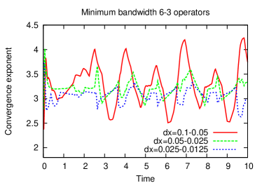
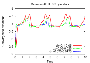
Figure 2: Convergence exponents for the minimum bandwidth (top) and the minimum ABTE (bottom) $D_{6-3}$ operators.

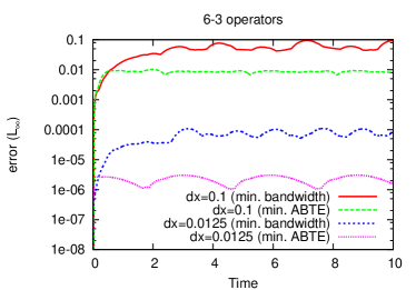
Figure 3: Accuracy comparison between the $D_{6-3}$ operators of the previous figure. For the highest resolution that we used, the errors with the minimum average boundary truncation error operator are around two orders of magnitude smaller than those obtained with the minimum bandwidth one.

We conjecture that this is caused by larger truncation errors for this operator near boundaries. This is unfortunately not immediately evident when looking at the boundary error coefficients $c_{i}$ or the ABTE. However, three of the inner four error coefficients have absolute values less than $0.1$ for the optimized operator, whereas this is the case for only 1 error coefficient for the standard operator. The fact that the accuracy is also higher with the optimized operator also points to the fact that the standard operator introduces somehow a much larger error.

As a summary, the minimum ABTE operator is the preferred choice in this case, the minimum bandwidth $D_{6-3}$ operator does not have a large spectral radius in comparison, but it does have much larger truncation error coefficients.

The operator $D_{8-4}$.

Figure 4 shows the results of similar convergence tests, also in the $L_{\infty}$ norm, for the $D_{8-4}$ operators. As discussed in the previous Section, in this case the minimum bandwidth operator has both very large spectral radius and truncation error coefficients, so large that it is actually not worthwhile presenting here details of simulations using it (they actually crash unless a very small Courant factor is used, as expected). In references Lehner et al. (2005) and Svärd et al. (2005) two different sets of parameters were found, both of which reduced the spectral radius by around one order of magnitude, when compared to the minimum bandwidth one. Here we concentrate on comparing an operator constructed in a similar way (with slightly smaller spectral radius than the ones of Lehner et al. (2005); Svärd et al. (2005)) —that is, minimizing the spectral radius— with the minimum ABTE operator. We see that in both cases we find a global convergence exponent close to five. Figure 5 shows at fixed resolution (with the highest resolution that we used for the convergence tests) a comparison between these two operators, by displaying the errors with respect to the exact solution, in the $L_{\infty}$ norm. There is an improvement of a factor of two in the minimum ABTE case (as mentioned, the differences with the minimum bandwidth case are much larger). Notice also that even though not at round-off level, the errors in our simulations are quite small, of the order of $10^{-7}$ in the $L_{\infty}$ norm (in the $L_{2}$ norm they are almost an order of magnitude smaller).

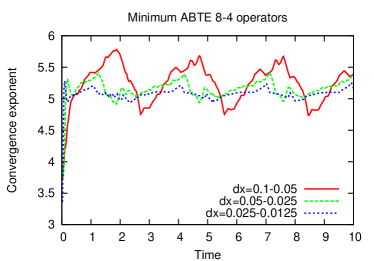
Figure 4: Convergence exponents for the minimum spectral radius (top) and the minimum ABTE (bottom) $D_{8-4}$ operators.

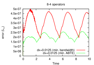
Figure 5: Comparison of the accuracy of the two $D_{8-4}$ operator types shown in the previous figure in the $L_{\infty}$ norm. Although both operators have quite similar error coefficients, there is up to a factor of two difference in the errors seen in the actual runs.

V.2 Operators based on a restricted full norm

V.2.1 Operator properties

Let us now consider operators that are based on a restricted full norm (see Section II.1). In this case the norm always depends on the free parameters, and it is not necessarily positive definite for all values of them. Therefore these free parameters are subject to the constraint of defining a positive definite norm.

We examine here the operators $D_{4-3}$, $D_{6-5}$, and $D_{8-7}$. These operators have five, seven and nine boundary points, respectively, and their maximum stencil size are seven, ten and thirteen points, respectively.

The family of $D_{4-3}$ operators has three independent parameters, and as mentioned above, they have to be chosen so that the corresponding norm is positive definite.

We constructed operators by minimizing their bandwidth, their spectral radius, and their average boundary truncation error. In minimizing the bandwidth there is some arbitrariness in the choice as to which coefficients in the stencils are set to zero. Here we follow Strand (1994) and set the coefficients $q_{1,5}$, $q_{2,7}$, and $q_{3,7}$ to zero, where the first index labels the stencil starting with 1 from the boundary and the second index labels the point in the stencil. This results in two solutions, but only one of them corresponds to a positive definite norm.

A comparison of the spectral radius, ABTE, and error coefficients is listed in table 6.

Table 6: Properties of the restricted full norm $D_{4-3}$ operators.

	Minimum	Minimum	Minimum
Operator	bandwidth	spectral radius	ABTE
Spectral radius	$2.428$	$1.322$	$2.758$
ABTE	$0.1281$	$0.5824$	$0.0230$
$c_{1}$	$0.2500$	$1.2359$	$-0.0100$
$c_{2}$	$-0.1333$	$-0.2378$	$-0.0409$
$c_{3}$	$0.0201$	$-0.3166$	$0.0251$
$c_{4}$	$0.0366$	$0.1053$	$-0.0086$
$c_{5}$	$-0.0065$	$0.0279$	$-0.0129$

We find in our simulations (see below) that the minimum bandwidth and the minimum ABTE $D_{4-3}$ operators have very similar properties. The latter, however, has slightly smaller errors, enough to offset the slightly smaller time steps required for stability. The operator with a minimum spectral radius unfortunately has very large errors; in fact, we have not been able to stabilize the system with any amount of artificial dissipation when we used this operator for equations with non-constant coefficients in 3D.

The family of $D_{6-5}$ operators has four independent parameters that again have to be chosen so that the norm is positive definite. For the minimal bandwidth operator we choose to zero the coefficients $q_{1,7}$, $q_{2,9}$, $q_{2,10}$ and $q_{3,10}$. The resulting equations cannot be solved analytically, but numerically we find eight solutions, of which four are complex. From the remaining real solutions only one of them results in a positive definite norm. A comparison between the properties of the minimal bandwidth, minimal spectral radius and minimal ABTE operators is listed in table 7.

Table 7: Properties of the restricted full norm $D_{6-5}$ operators.

	Minimum	Minimum	Minimum
Operator	bandwidth	spectral radius	ABTE
Spectral radius	$2.940$	$1.458$	$3.194$
ABTE	$0.0986$	$0.5380$	$0.0648$
$c_{1}$	$0.1667$	$1.3692$	$-0.0154$
$c_{2}$	$-0.1558$	$-0.2682$	$-0.0507$
$c_{3}$	$0.0672$	$-0.2118$	$0.1336$
$c_{4}$	$0.0953$	$0.0097$	$0.0532$
$c_{5}$	$-0.0433$	$0.0702$	$-0.0733$
$c_{6}$	$0.0141$	$0.1434$	$0.0187$
$c_{7}$	$-0.0163$	$-0.0972$	$-0.0123$

As in the $D_{4-3}$ case, the minimum spectral radius operator has a much smaller spectral radius than the other ones but, again, we did not manage to stabilize it with dissipation (at least, with reasonable amounts of it) in the 3D case with non-constant coefficients. The errors for the minimum ABTE operator are significantly smaller than the minimum bandwidth one, which is reflected in practice by smaller errors; in addition, the operator could be stabilized with significantly less artificial dissipation.

It should be noted at this point that we did not manage to stabilize the $D_{6-5}$ operator with a naive adapted Kreiss–Oliger like dissipation prescription. We tried applying Kreiss–Oliger dissipation in the interior of the domain, and applying no dissipation near the boundary where the centered stencils cannot be applied. This failed. Presumably this is caused by the fact that the dissipation operator is not negative semi-definite with respect to the SBP norm. Only after constructing boundary dissipation operators following the approach of Ref. Mattsson et al. (2004), did we arrive at a stable scheme involving the $D_{6-5}$ operator.

The family of $D_{8-7}$ operators has five independent parameters. When attempting to obtain minimum bandwidth operators by setting the coefficients $q_{1,9}$, $q_{2,11}$, $q_{2,12}$, $q_{2,13}$, and $q_{3,13}$ to zero, we numerically find 24 solutions, of which 16 are complex and 8 are real. However, none of these solutions yields a positive definite norm. The minimum spectral radius operator has so large error coefficients that we could not stabilize it with reasonable amounts of dissipation in the 3D non-constant coefficient case. The minimum ABTE operator has a spectral radius larger than 60000 and so would require very small time steps when explicit time evolution is used.

Since none of the operators considered so far was usable in practice, we experimented with several other ways of choosing the parameters. First, we tried to minimize a weighted average of the spectral radius and ABTE for different weight values, but none of these operators turned out to be useful, even though their properties were much improved. By minimizing the sum of the squares of the difference between error coefficients in neighboring boundary points, we next attempted to reduce the noise produced in the boundary region. Even when weighted with the spectral radius, these operators proved not to be an improvement. Finally, based on the observation that some choices of parameters lead to very large values in the inverse of the norm, which directly affects the dissipation operator near the boundary (see Eq. (10)), we speculated that for some parameter sets the dissipation operator might make things worse near the boundary, and experimented with choosing parameters that would minimize the condition number of the norm in combination with any of the previously mentioned properties.

However, even though we were able to find parameter sets that looked reasonable with respect to spectral radius, error coefficients and properties of the norm, none of the operators that we constructed could be stabilized with any amount of dissipation in the 3D non-constant coefficient case. This is presumably related to some important properties not holding in the non-diagonal case, as discussed in Section II.2. Of course, it could still happen that usable $D_{8-7}$ operators do exist, using some other criteria to choose parameters.

V.2.2 Numerical tests

For the restricted full operators we usually have to add dissipation. There are several causes for this, which are well understood; we have reviewed them in Section II.

The operator $D_{4-3}$.

One main driving point behind using operators based on non-diagonal norms is that their order of accuracy near the boundary is higher. Our operators based on restricted full norms drop one order of accuracy near the boundary, which means that the global convergence order is, in theory, not affected. (See the standard $D_{6-3}$ operator, described in Section V.1.2, and illustrated in Figure 2, for an example where this is false in practice.)

Figure 6 shows the results of convergence tests in the $L_{\infty}$ norm for $D_{4-3}$ operators, for both the minimum bandwidth and the new, optimized, minimum ABTE operator. In both cases the global convergence exponent is very close to four. Different from the operators based on diagonal norms, the convergence order is also almost constant in time. This may be so because the boundary is here not the main cause of discretization error, so that the resulting accuracy is here independent of what kind of feature of the solution is currently propagating through the boundary.

Figure 7 compares the two $D_{4-3}$ operators at a fixed, high resolution. The two operators lead to very similar $L_{\infty}$ norms of the solution error. This difference in accuracy is much smaller than it was for the operators based on diagonal norms. Altogether, the optimization leads to no practical advantage.

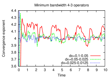
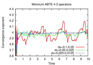
Figure 6: Convergence exponents for the minimum bandwidth (top) and the minimum ABTE (bottom) $D_{4-3}$ operators.

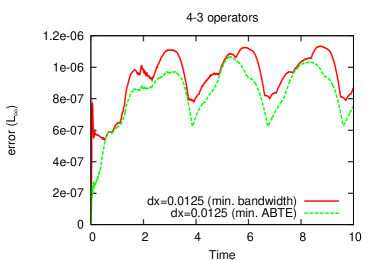
Figure 7: Accuracy comparison of the two types of $D_{4-3}$ operators shown in the previous figure in the $L_{\infty}$ norm. Contrary to the results for the $D_{6-3}$ and $D_{8_{4}}$, here the difference in errors is minimal.

The operator $D_{6-5}$.

The operator $D_{6-5}$ is expected to have the highest global order of accuracy of all the operators discussed in this paper (since we were not able to stabilize the $D_{8-7}$ operator with dissipation). We do in fact see sixth order convergence, but only when using a sufficiently accurate time integration scheme. Figure 8 shows the results of convergence tests in the $L_{\infty}$ norm for the new, optimized $D_{6-5}$ operator with dissipation, using a Courant factor $\lambda=0.25$, for both fourth and sixth order accurate Runge–Kutta time integrators (RK4 and RK6).

When RK4 is used, the convergence exponent drops from about $6$ to close to $5$ for our highest resolution. This effect is not present when we use RK6, indicating that it is the time integrator’s lower convergence order that actually poisons the results when resolution is increased.

Figure 8: Convergence for the optimized $D_{6-5}$ operator with dissipation and Runge–Kutta time integrators of order four (top) and six (bottom), respectively. We see a slightly lower convergence order for the highest resolution when RK4 is used. This effect is not present with the RK6 integrator. The lower convergence order indicates that the accuracy of the spatial finite differencing operators is high enough, so that the overall error is dominated by the accuracy of the time integrator.

Instead of using a higher order time integrator, it would also have been possible to reduce the time step size. Especially in complicated geometries, an adaptive step size control is very convenient; this lets one specify the desired time integration error, and the step size is automatically adjusted accordingly.

V.3 Comparison between operators

V.3.1 Comparison of accuracy

We now compare the operators based on a diagonal and on a restricted full norm that we described and examined above. Figure 9 shows, for two different resolutions, the solution errors for all our new operators. As one can see, our best performing operators are $D_{8-4}$ and $D_{6-5}$ . One can also see that, for the highest resolution shown there, which corresponds to $161^{3}$ grid points per block, there is a difference of five orders of magnitude between the errors of $D_{6-5}$ and $D_{2-1}$. This demonstrates nicely the superiority of our new high order operators when a high accuracy is desired.

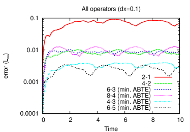
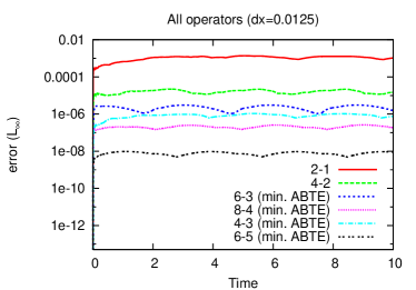
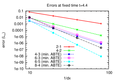
Figure 9: Comparison of the errors for all the new, optimized, differencing operators constructed in this paper. The top (middle) plot shows a comparison of all the unique and optimized operators at low (high) resolutions. The bottom plot shows the error at $t=4.4$ for all resolutions. The most successful operators are the optimized $D_{6-5}$, $D_{4-3}$, and $D_{8-4}$.

Even for the lowest resolution shown here, which uses only $21^{3}$ grid points per block, the difference is still more than one order of magnitude, indicating that $D_{6-5}$ or $D_{4-3}$ would be fine choices there.

V.3.2 Comparison of cost

Higher order operators allow higher accuracy with the same number of grid points, but they also require more operations per grid point and thus have a higher cost. Table 8 compares actual run times per time integrator step for runs with $161^{3}$ grid points per block. These measured costs include not only calculating the right hand side, which requires taking the derivatives, but also applying the boundary conditions, which requires decomposing the system into its characteristic modes, and also some inter-processor communication. The time spent in the time integration itself is negligible.

Table 8: Relative operator costs for our test problem, measured in seconds per time step with an RK4 integrator. The number in parentheses for the $D_{6-5}$ used an RK6 time integrator, which requires seven iterations instead of four. The numbers marked with an asterisk were obtained from runs using a larger number of processors and are probably larger than they would be otherwise due to scaling inefficiencies.

	Time [sec]	Time [sec]
Operator	without dissipation	with dissipation
$D_{2-1}$	$26.9$	$27.7$
$D_{4-2}$	$27.9$	$29.7$
$D_{6-3}$	$30.5$	$32.0$
$D_{8-4}$	$34.4$	$35.3$
$D_{4-3}$	$28.6$	$44.8$
$D_{6-5}$	$41.6^{*}$	$39.1\;(86.2^{*})$

Larger stencils increase the cost slightly. This increase in cost is more than made up by the increase in accuracy, as shown above. For operators based on diagonal norms, adding dissipation to the system increases the cost only marginally. The dissipation operators for derivatives based on non-diagonal norms are more complex to calculate and increase the run time noticeably. All numbers were obtained from a straightforward legible implementation in Fortran, without spending much effort on optimizing the code for performance.

The effect of higher order operators on the overall run time is not very pronounced. As they do not increase the storage requirements either, the only reason speaking against using them (for smooth problems) seems to be the effort one has to spend constructing and implementing them.

VI Conclusion

Let us summarize the main points of this paper. We have explicitly constructed accurate, high-order finite differencing operators which satisfy summation by parts. This construction is not unique, and it is necessary to specify some free parameters. We have considered several optimization criteria to define these parameters; namely, (a) a minimum bandwidth, (b) a minimum of the truncation error on the boundary points, (c) a minimum spectral radius, and a combination of these.

We examined in detail a set of operators that are up to tenth order accurate. We found that minimum bandwidth operators may have a large spectral radius or truncation error near the boundary. Optimizing for these two criteria can, surprisingly, reduce the operators’ spectral radius by three orders and their accuracy near the boundary by two orders of magnitude.

Some of the finite differencing operators require artificial dissipation. We have therefore also constructed high-order dissipation operators, compatible with the above finite differencing operators, and also semi-definite with respect to the SBP scalar product.

We tested the stability and accuracy of these operators by evolving a scalar wave equation on a spherical domain. Our domain is split into seven blocks, each discretized with a structured grid. These blocks are connected through penalty boundary conditions. We demonstrated that the optimized finite differencing operators have also far superior properties in practice. The most accurate operators are $D_{8-4}$ and $D_{6-5}$; the latter is in our setup five orders of magnitude more accurate than a simple $D_{2-1}$ operator.

Appendix A Operator coefficients

We provide, for the reader’s convenience, the coefficients for the derivative and dissipation operators that we constructed above. Since the values of these coefficients themselves are only of limited interest, and since there is a large danger of introducing errors when typesetting these coefficients, we make them available electronically instead. We also make a Cactus cac thorn SummationByParts available via anonymous CVS. This thorn implements the derivative and dissipation operators. Our web pages num contain instructions for accessing these. For the sake of continuity, we will also make the coefficients available on www.arxiv.org together with this article.

We distribute the coefficients as a set of files, where each file defines on operator. The content of the file is written in a Fortran-like pseudo language that defines the coefficients in declarations like

  a(1) = 0.5
  q(2,3) = 42.0

and sometimes makes use of additional constants, as in

  x1 = 3
  a(2) = x1 + 4

We write here a(1) as $a_{1}$ and q(2,3) as $q_{23}$.

A.1 Derivative operators

The derivative operators $D_{2-1}$, $D_{4-2}$, $D_{6-3}$, $D_{8-4}$, $D_{4-3}$, and $D_{6-5}$ are defined via coefficients $a_{i}$ and $q_{ij}$. In the interior of the domain it is

$$D_{ij}u_{j} = \frac{1}{h}\sum_{j=1}^{s}a_{j}\left(u_{i+j}-u_{i-j}\right)$$ (24)

and near the left boundary it is (i.e. $i=1,b$)

$$D_{ij}u_{j} = \frac{1}{h}\sum_{j=1}^{s}q_{ji}u_{j}.$$ (25)

At the right boundary the same coefficients are used in opposite order and with opposite sign.

A.2 Dissipation operators

A.2.1 Dissipation operators based on diagonal norms

The dissipation operators corresponding to $D_{2-1}$, $D_{4-2}$, $D_{6-3}$, and $D_{8-4}$ are defined via coefficients $a_{ij}$ and $q_{i}$.

In the interior of the domain it is

$$A_{ij}u_{j} = \frac{\epsilon}{2^{2p}}\left[q_{0}u_{i}+\sum_{j=1}^{s}q_{j}\left(u_{i-j}+u_{i+j}\right)\right]$$ (26)

and near the boundary it is

$$A_{ij}u_{j} = \frac{\epsilon}{2^{2p}}\sum_{j=1}^{s}a_{ji}u_{j},$$ (27)

where $\epsilon\geq 0$ selects the amount of dissipation and is usually of order unity.

A.2.2 Dissipation operators based on non-diagonal norms

The dissipation operators corresponding to $D_{4-3}$ and $D_{6-5}$…are more complicated, since they depend on the user parameters specifying the number of grid points, $N$, and the size of the transition region (i.e. the region where $B_{p}$ is different from 1).

The dissipation operators are then constructed according to Eq. (10)

$$A_{2p}=-\frac{\epsilon}{2^{2p}}\,h^{2p}\;\Sigma^{-1}D_{p}^{T}B_{p}D_{p}.$$ (28)

The coefficients for the inverse of the norm, $\Sigma^{-1}$, are provided in the boundary region only. In the files this inverse is denoted by sigma(i,j). In the interior the norm (and its inverse) is diagonal with value $1$.

In the $D_{4-3}$ case, the $N\times N$ matrix $D_{2}$ defining the consistent approximation of $d^{2}/dx^{2}$ is given by

$$D_{2}=\frac{1}{h^{2}}\left(\begin{array}[]{rrrrcrrrr}1&-2&1&0&&&&&\\ 1&-2&1&0&&&&&\\ 0&1&-2&1&&&&&\\ &&&&\ddots&&&&\\ &&&&&1&-2&1&0\\ &&&&&0&1&-2&1\\ &&&&&0&1&-2&1\end{array}\right),$$ (29)

while the diagonal matrix $B_{2}$ has the value $h$ at either boundary and increases linearly to the value 1 across the user defined transition region.

In the $D_{6-5}$ case the matrix defining the consistent approximation of $d^{3}/dx^{3}$ near the left boundary $D_{3}^{l}$ is

$$D_{3}^{l}=\frac{1}{h^{3}}\left(\begin{array}[]{rrrrrc}-1&3&-3&1&0&\\ -1&3&-3&1&0&\\ -1&3&-3&1&0&\\ 0&-1&3&-3&1&\\ &&&&&\ddots\end{array}\right),$$ (30)

while at the right boundary $D_{3}^{r}$ is

$$D_{3}^{r}=\frac{1}{h^{3}}\left(\begin{array}[]{crrrrr}\ddots&&&&&\\ &-1&3&-3&1&0\\ &0&-1&3&-3&1\\ &0&-1&3&-3&1\\ &0&-1&3&-3&1\end{array}\right).$$ (31)

Since the values on the diagonal in the interior of $D_{3}^{l}$ and $D_{3}^{r}$ are $-3$ and $3$, respectively, it is impossible to construct a single matrix $D_{3}$ to cover the whole domain. However, since both matrix products $(D_{3}^{l})^{T}D_{3}^{l}$ and $(D_{3}^{r})^{T}D_{3}^{r}$ result in the same interior operator, dissipation operators can be constructed in the left and right domain separately and then combined into a global operator. The diagonal matrix $B_{3}$ has the values $h^{2}$ at the boundary and and $1$ in the interior, and a third order polynomial with zero derivative at either end of the transition region is used to smoothly connect the boundary with the interior.

References

- Kreiss and Scherer (1974) H. O. Kreiss and G. Scherer, in Mathematical Aspects of Finite Elements in Partial Differential Equations, edited by C. D. Boor (Academica Press, New York, 1974).
- Kreiss and Scherer (1977) H. O. Kreiss and G. Scherer, Tech. Rep., Dept. of Scientific Computing, Uppsala University (1977).
- Olsson (1995a) P. Olsson, Math. Comp. 64, 1035 (1995a).
- Olsson (1995b) P. Olsson, Math. Comp. 64, S23 (1995b).
- Olsson (1995c) P. Olsson, Math. Comp. 64, 1473 (1995c).
- Carpenter et al. (1994) M. Carpenter, D. Gottlieb, and S. Abarbanel, J. Comput. Phys. 111, 220 (1994).
- Gustafsson (1998) B. Gustafsson, BIT 38, 293 (1998).
- Mattsson (2003) K. Mattsson, J. Sci. Comput. 18, 133 (2003).
- Strand (1996) B. Strand, Ph.D. thesis, Uppsala University, Department of Scientific Computing, Uppsala University. Uppsala, Sweden (1996).
- Carpenter et al. (1999) M. Carpenter, J. Nordström, and D. Gottlieb, J. Comput. Phys. 148, 341 (1999).
- Nordström and Carpenter (2001) J. Nordström and M. Carpenter, J. Comput. Phys. 173, 149 (2001).
- Reula (1998) O. Reula, Living Rev. Rel. 1, 3 (1998), URL http://relativity.livingreviews.org/Articles/lrr-1998-3/index%.html.
- Rauch (1985) J. Rauch, Trans. Am. Math. Soc. 291, 167 (1985).
- Secchi (1996a) P. Secchi, Differential Integral Equations 9, 671 (1996a).
- Secchi (1996b) P. Secchi, Arch. Rat. Mech. Anal. 134, 155 (1996b).
- Lehner et al. (2005) L. Lehner, O. Reula, and M. Tiglio, to appear in Class. Quantum Grav. (2005), eprint gr-qc/0507004.
- Svärd et al. (2005) M. Svärd, K. Mattsson, and J. Nordström, J. Sci. Comput. 24, 79 (2005).
- Mattsson et al. (2004) K. Mattsson, M. Svärd, and J. Nordström, J. Sci. Comput. 21, 57 (2004).
- Friedrich (2002) H. Friedrich, Lect. Notes Phys. 604, 1 (2002), eprint gr-qc/0209018.
- Strand (1994) B. Strand, J. Comput. Phys. 110, 47 (1994).
- Tadmor (1994) E. Tadmor, in Lecture notes delivered at Ecole des Ondes, "Méthodes numériques d’ordre élevé pour les ondes en régime transitoire", INRIA–Rocquencourt January 24-28. (1994), URL http://www.cscamm.umd.edu/people/faculty/tadmor/pub/spectral-%approximations/Tadmor.INRIA-94.pdf.
- Svärd (2005) M. Svärd, to appear in J. Sci. Comput. (2005).
- Goodale et al. (2003) T. Goodale, G. Allen, G. Lanfermann, J. Massó, T. Radke, E. Seidel, and J. Shalf, in Vector and Parallel Processing - VECPAR’2002, 5th International Conference, Lecture Notes in Computer Science (Springer, Berlin, 2003), URL http://www.cactuscode.org.
- (24) Cactus Computational Toolkit home page, URL http://www.cactuscode.org/.
- Schnetter et al. (2004) E. Schnetter, S. H. Hawley, and I. Hawke, Class. Quantum Grav. 21, 1465 (2004), eprint gr-qc/0310042.
- (26) Mesh Refinement with Carpet, URL http://www.carpetcode.org/.
- (27) B. Zink, P. Diener, E. Pazos, and M. Tiglio, submitted to PRD, eprint gr-qc/0511163.
- (28) LAPACK: Linear Algebra Package, URL http://www.netlib.org/lapack/.
- (29) BLAS: Basic Linear Algebra Subroutines, URL http://www.netlib.org/blas/.
- (30) Netlib Repository, URL http://www.netlib.org/.
- Burns et al. (1994) G. Burns, R. Daoud, and J. Vaigl, in Proceedings of Supercomputing Symposium (1994), pp. 379–386, URL http://www.lam-mpi.org/download/files/lam-papers.tar.gz.
- Squyres and Lumsdaine (2003) J. M. Squyres and A. Lumsdaine, in Proceedings, 10th European PVM/MPI Users’ Group Meeting (Springer-Verlag, Venice, Italy, 2003), no. 2840 in Lecture Notes in Computer Science, pp. 379–387.
- (33) LAM: LAM/MPI Parallel Computing, URL http://www.lam-mpi.org/.
- Gropp et al. (1996) W. Gropp, E. Lusk, N. Doss, and A. Skjellum, Parallel Computing 22, 789 (1996).
- Gropp and Lusk (1996) W. D. Gropp and E. Lusk, User’s Guide for mpich, a Portable Implementation of MPI, Mathematics and Computer Science Division, Argonne National Laboratory (1996), aNL-96/6.
- mpi (a) MPICH: ANL/MSU MPI implementation, URL http://www-unix.mcs.anl.gov/mpi/mpich/.
- mpi (b) MPI: Message Passing Interface Forum, URL http://www.mpi-forum.org/.
- (38) Sonderforschungsbereich/Transregio 7 “Gravitational Wave Astronomy”, URL http://www.tpi.uni-jena.de/SFB/.
- (39) CCT Numerical Relativity, URL http://www.cct.lsu.edu/about/focus/numerical/.