A Study of the Edge-Switching Markov-Chain Method for the Generation of Random Graphs

Abstract

We study the problem of generating connected random graphs with no self-loops or multiple edges and that, in addition, have a given degree sequence. The generation method we focus on is the edge-switching Markov-chain method, whose functioning depends on a parameter $w$ related to the method’s core operation of an edge switch. We analyze two existing heuristics for adjusting $w$ during the generation of a graph and show that they result in a Markov chain whose stationary distribution is uniform, thus ensuring that generation occurs uniformly at random. We also introduce a novel $w$-adjusting heuristic which, even though it does not always lead to a Markov chain, is still guaranteed to converge to the uniform distribution under relatively mild conditions. We report on extensive computer experiments comparing the three heuristics’ performance at generating random graphs whose node degrees are distributed as power laws.

Keywords: Random-graph generation, Edge switch, Markov chain.

1 Introduction

Let $D=\{d_{1},d_{2},\ldots,d_{n}\}$ be a set of nonnegative integers such that $d_{1}\geq d_{2}\geq\cdots\geq d_{n}$ and let ${\cal G}_{D}$ be the set of all connected graphs on $n$ nodes that have no self-loops or multiple edges and for which $D$ is the degree sequence. That is, the degree of node $u_{j}$, $1\leq j\leq n$, is $d_{j}$. We know from [11, 7] that ${\cal G}_{D}$ is a nonempty set, in which case we say that $D$ is realizable, if and only if all the following conditions hold:

• $\sum_{j=1}^{n}d_{j}$ is even.

• $\sum_{j=1}^{n}d_{j}\geq 2(n-1)$.

• $\sum_{j=1}^{k}d_{j}\leq k(k-1)+\sum_{j=k+1}^{n}\min\{k,d_{j}\}$ for all $k$ such that $1\leq k\leq n$.

We consider in this paper the problem of generating graphs of ${\cal G}_{D}$ uniformly at random when $D$ is realizable.

In the absence of the connectivity constraint, the problem of generating random graphs for a given degree sequence is closely related to some other problems, like generating a $(0,1)$ matrix with given marginals [25], approximating the permanent of a matrix [19], and sampling a perfect matching or an $f$-factor of a graph [14, 5]. However, it remains generally unknown how to generate graphs uniformly at random for a given degree sequence within reasonable time bounds [26], even though exceptions exist for some special cases, like regular [21] and bipartite graphs [14, 19].

The problem of generating random graphs has recently acquired considerable prominence from a practical perspective. Since many real-world networks, like the Internet, the WWW, social networks, and scientific-collaboration networks, typically have a very large number of nodes and have evolved over time in such an unorganized way that only limited information is known about their topologies [3, 24], many studies of their properties have been conducted within a random-graph framework [2, 15]. In addition, these networks are now known to differ sharply from the classical random-graph model introduced by Erdős and Rényi [12, 8], in which the node-degree distribution is the Poisson distribution. Some empirical studies suggest that many of them have node-degree distributions that seem to conform to a power law [13, 6, 3, 24], that is, the probability that a randomly chosen node has degree $a$ is proportional to $a^{-\tau}$ for some $\tau>1$.

Clearly, any method for sampling a graph uniformly at random from ${\cal G}_{D}$ for a given $D$ can be easily extended to generate random graphs having a power-law node-degree distribution. We first obtain $D$ by sampling each $d_{j}$ from the power-law distribution. If $D$ turns out not to be realizable, then we discard it entirely and obtain a new one, repeating this process while needed. We then select the desired graph uniformly at random from ${\cal G}_{D}$.

Other, more complex methods for generating random graphs having node degrees distributed as a power law have been proposed. In these methods, generation is achieved by successively adding nodes and edges to the graph in such a way that tries to follow some principles, like preferential attachment, that are believed to have guided the evolution of some real-world networks [22, 9]. However, simply generating a graph having a given degree sequence sampled from the power-law distribution has been observed to perform satisfactorily with regard to certain measures [27]. Moreover, this approach can be used to obtain random graphs having any node-degree distribution, which is an important flexibility since correctly determining the node-degree distribution of real-world networks has remained essentially an open problem [1].

Given a realizable $D$, we consider the generation method that we call the edge-switching Markov-chain (ESMC) method for choosing graphs from ${\cal G}_{D}$ uniformly at random, also variously known by other denominations [16]. This method, which can be modeled as a Markov chain and whose details are more thoroughly described in Section 2, employs an operation that we call an edge switch to transform a graph of ${\cal G}_{D}$ into another graph, maybe not in ${\cal G}_{D}$ by virtue of not being connected, that has the same degree sequence $D$. Let $G$ be the graph being generated. To avoid generating unconnected graphs, we periodically perform a connectivity test on $G$. If $G$ is unconnected, we undo all the edge switches performed since the previous connectivity test. Basically, the method consists of first obtaining a graph $G$ from ${\cal G}_{D}$ deterministically and then applying a series of edge switches and connectivity tests to $G$ until a certain halting condition is satisfied. We also discuss in Section 2 a methodology for obtaining the halting condition, which ultimately also embodies a criterion for estimating how close $G$ is to a uniformly random sample from ${\cal G}_{D}$.

The ESMC method is intrinsically based on an integer parameter $w\geq 1$ giving the number of edge switches to be attempted between successive connectivity tests. Naturally, setting $w$ appropriately is crucial to the performance of the method. When $w$ is too small, a large number of connectivity tests is performed, which dramatically increases the running time of the method, as the time complexity of a connectivity test is high in comparison to the time complexity of an edge switch. On the other hand, when $w$ is excessively large the probability that the connectivity test is performed on an unconnected graph tends to be high, possibly causing many edge switches to be undone. Obtaining an ideal value for $w$ beforehand seems to be an elusive goal, so heuristics have been proposed for adjusting $w$ along the algorithm’s execution [16, 29]. We discuss the existing heuristics, and also introduce a new one, in Section 3.

We present in Section 4 the results of extensive computer experiments for degree sequences sampled from power-law distributions. We evaluate the three heuristics described in Section 3 along with two different halting conditions. In general, our computational results indicate that, on average, our heuristic outperforms the two existing heuristics in terms of the total running time by a margin of $12\%$ to $86\%$. We conclude in Section 5.

2 The ESMC method

We henceforth denote by $G$ the graph being generated, that is, the graph on which the edge switches and the connectivity tests are performed. An edge switch is performed on a pair of nonadjacent edges (i.e., edges that share no nodes) and consists of removing them from $G$ and adding back one of two other pairs of edges. The pair of edges to be added to $G$ is chosen at random from these two and the edge switch is only carried through if neither edge of the chosen pair already exists in $G$. For example, let $(u_{j},u_{k})$ and $(u_{x},u_{y})$ be two nonadjacent edges of $G$. The edge-switching operation on $(u_{j},u_{k})$ and $(u_{x},u_{y})$ consists of removing these edges from $G$ and adding to $G$ either $(u_{j},u_{x})$ and $(u_{k},u_{y})$ or $(u_{j},u_{y})$ and $(u_{k},u_{x})$. Although node degrees are clearly seen to remain unchanged by an edge switch, $G$ may become an unconnected graph. Figure 1(a) illustrates the two possible edges switches on the edges $(u_{j},u_{k})$ and $(u_{x},u_{y})$. Figure 1(b) illustrates a situation in which only one edge switch can be carried through on those edges.

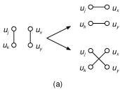
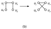
Figure 1: The two possible edge switches on the edges $(u_{j},u_{k})$ and $(u_{x},u_{y})$ (a) and a scenario in which only one of them can be carried through (b).

The ESMC method is best described on a Markov chain ${\cal M}$ having one state associated with each graph of ${\cal G}_{D}$. If $G_{1},G_{2},\ldots,G_{\left|{\cal G}_{D}\right|}$ are the graphs in ${\cal G}_{D}$ and $X_{1},X_{2},\ldots,X_{\left|{\cal G}_{D}\right|}$ are the states of ${\cal M}$, then we let, for $1\leq i\leq\left|{\cal G}_{D}\right|$, $X_{i}$ be the state in which $G=G_{i}$. In essence, the ESMC method consists of initially obtaining a graph of ${\cal G}_{D}$ and then performing a sequence of transitions on ${\cal M}$ from the corresponding state until a certain halting condition is satisfied.

In order to obtain the initial graph, we employ the Havel-Hakimi algorithm [18, 17, 7], which successively adds edges to an initial graph $G$ having $n$ isolated nodes. For $1\leq j\leq n$, along the process let the residual degree $r_{j}$ of $u_{j}$ be the difference between $d_{j}$ and the number of edges already incident to $u_{j}$; clearly, $r_{j}=d_{j}$ initially. The algorithm repeatedly selects the node, say $u_{k}$, having the highest residual degree and connects it to the $r_{k}$ nodes having the next highest residual degrees, which leads to $r_{k}=0$ and also to smaller values of the other nodes’ residual degrees. The repetition goes on until $r_{j}=0$ for all $j$ such that $1\leq j\leq n$. At this moment, $G$ has degree sequence $D$ but may be unconnected. Since $D$ is realizable, $G$ must contain a cycle if it is not connected. If we take an edge of this cycle and an edge of another connected component, and perform an edge switch on them, then necessarily two of the connected components of $G$ are merged together into a single one. This process can be repeated until $G$ becomes connected.

Let us then describe what constitutes a transition in ${\cal M}$. Let $w\geq 1$ be an integer parameter. A transition in ${\cal M}$ is a sequence of $w$ steps that we call edge-switching attempts. In each edge-switching attempt, we randomly select two distinct edges of $G$. If they are not adjacent, then we randomly choose one of the two possible edge switches. If the chosen edge switch is feasible, that is, it does not involve adding an edge that already exists in $G$, then we go on and perform the edge switch. $G$ is kept unchanged otherwise. After $w$ edge-switching attempts, we perform a connectivity test on $G$. If $G$ turns out to be unconnected, then we undo all the edge switches performed during the previous $w$ edge-switching attempts.

Now let $m$ be the number of edges of $G$. If we use an array with the edges of the graph, an adjacency matrix, and an appropriate collection of incidence lists and pointers, then an edge switch can be done in $O(1)$ time while requiring $\Theta(n^{2})$ space, which for large $n$ is prohibitive. An alternative way is to use an array with the edges of the graph and an appropriate collection of incidence trees and pointers, which leads to $O(\log d_{1})$ time and $\Theta(m)$ space instead. This has been our choice in all the computer experiments we discuss in Section 4. In any case, and considering that the connectivity test can be performed in $O(m)$ time, setting $w$ properly is essential to the achievement of good performance. We return to this issue in Section 3.

In ${\cal M}$, a transition exists from $X_{i}$ to $X_{j}$, $1\leq i,j\leq\left|{\cal G}_{D}\right|$, if and only if there is a sequence of $w$ edge-switching attempts transforming $G_{i}$ into $G_{j}$. Let $p_{i,j}$ be the probability associated with this transition. Clearly, $p_{i,j}=p_{j,i}$ so long as $w$ is constant (every edge switch can be undone with the same probability with which it was previously done), and $p_{i,i}>0$ (every edge-switching attempt may select adjacent edges to switch or an infeasible edge switch). The main results that pertain to the use of ${\cal M}$ in sampling a random graph from ${\cal G}_{D}$ uniformly at random are consequences of the following two classic theorems on Markov chains [20, 23].

Theorem 1.

A finite, irreducible, and aperiodic Markov chain converges to a unique stationary distribution regardless of the initial state.

Theorem 2.

Given a finite, irreducible, and aperiodic Markov chain with state space $\{Y_{1},Y_{2},\ldots,Y_{k}\}$, let $q_{i,j}$ be the probability associated with the transition from $Y_{i}$ to $Y_{j}$. If there are nonnegative numbers $\pi_{1},\pi_{2},\ldots,\pi_{k}$ such that $\sum_{i=1}^{k}\pi_{i}=1$, and furthermore

$$\pi_{i}q_{i,j}=\pi_{j}q_{j,i}$$

for all $i,j$ such that $1\leq i,j\leq k$, then the stationary distribution of this Markov chain is given by $\pi_{1},\pi_{2},\ldots,\pi_{k}$, with the probability associated with $Y_{i}$ being $\pi_{i}$, $1\leq i\leq k$.

Corollary 3, given next, follows directly from Theorem 2.

Corollary 3.

If $q_{i,j}=q_{j,i}$ for all $i,j$ such that $1\leq i,j\leq k$, then the stationary distribution of the Markov chain of Theorem 2 is the uniform distribution.

Our chain ${\cal M}$ is certainly finite and is also irreducible (since there is a sequence of transitions between any two states of ${\cal M}$ [28]) and aperiodic (since $p_{i,i}>0$ for all $i$ such that $1\leq i\leq\left|{\cal G}_{D}\right|$). Also, $p_{i,j}=p_{j,i}$ for all $i,j$ such that $1\leq i,j\leq\left|{\cal G}_{D}\right|$ if $w$ is constant. By Corollary 3, we then have the following.

Corollary 4.

If $w$ is constant, then ${\cal M}$ converges to the uniform distribution regardless of the initial state.

We finalize the section by discussing a halting condition for the ESMC method. For $t\geq 1$, let $g(t)$ be a function of $G$ right after the $t$th transition. Let also

$$\bar{g}(t)=\frac{g(0)+g(1)+\cdots+g(t)}{t+1},$$ (1)

where $g(0)$ refers to the initial $G$. The quantity in (1) is known to give an unbiased estimator of the expected value of $g(t)$ under the stationary distribution whenever Theorem 1 holds [20]. We use $\bar{g}(t)$ as an indirect indicator of the convergence of ${\cal M}$. Let $\delta\geq 1$ and $\gamma>0$ be two parameters, the former an integer. Our halting condition after the $t$th transition is that the inequality

$$\left|\frac{\bar{g}(z)-\bar{g}(t-\delta)}{\bar{g}(t-\delta)}\right|\leq\gamma$$ (2)

hold right after each of the $\delta$ most recent transitions that precede (with inclusion) the $t$th one (that is, for $t-\delta+1\leq z\leq t$). The efficacy of this halting condition depends clearly on the function $g(t)$. In Section 4 we present computational results for two different choices of $g(t)$ (deciding to halt based on one of them, however, bears no direct relationship to deciding to halt on the other).

3 Heuristics for parameter adjustment

As we remarked at the end of Section 1, adjusting $w$ along the evolution of ${\cal M}$ is a viable alternative, aiming at better convergence properties, to fixing its value at the onset. In this section we discuss some heuristics to do this. Each transition consists now of performing $w$ edge-switching attempts, a connectivity test (with the ensuing possible undoing of all the edge switches performed during the $w$ attempts), and moreover an update of the value of $w$. We consider two approaches to adjusting $w$. The first consists of a mechanism that is used in all existing heuristics for adjusting $w$ in accordance with the result of the previous connectivity test. The other one is a new heuristic that adjusts $w$ aiming at approximating a given probability for the success of the next connectivity test. Notice that, in either case, Corollary 4 is no longer applicable and the convergence of ${\cal M}$ has to be re-examined.

3.1 Two current heuristics

Let us begin with the first approach. We start with $w=1$ and increase the value of $w$ whenever the connectivity test succeeds; we decrease it otherwise. As we demonstrate next, a Markov chain exists associated with this approach that has a uniform stationary distribution.

Let ${\cal M}^{\prime}$ be a Markov chain whose states are each associated with a graph of ${\cal G}_{D}$ and a value of $w$. We denote by $X^{\prime}_{i,a}$ the state of ${\cal M}^{\prime}$ associated with $G_{i}$ and $w=a$. While ${\cal M}^{\prime}$ models the approach in question faithfully, it has more than one state associated with each graph of ${\cal G}_{D}$ and using it directly in our analysis may prove cumbersome. We then introduce another Markov chain, denoted by ${\cal M}^{\prime\prime}$ and having only $\left|{\cal G}_{D}\right|$ states, each associated with a graph of ${\cal G}_{D}$. We denote by $X^{\prime\prime}_{i}$ the state of ${\cal M}^{\prime\prime}$ associated with $G_{i}$. This state is the union of $X^{\prime}_{i,a}$ for all $a\geq 1$, i.e., $X^{\prime\prime}_{i}$ results from clustering together all the states of ${\cal M}^{\prime}$ that correspond to $G_{i}$.

In order to make the state space of ${\cal M}^{\prime}$ finite, we limit the value of $w$ by a fixed upper bound, henceforth denoted by $W$. This strategy not only makes ${\cal M}^{\prime}$ a finite Markov chain, which is crucial to the analysis that follows, but also avoids excessively large $w$ values, which may jeopardize the approach’s efficacy, especially in relation to the halting condition, as $g(t)$ may end up being calculated too sporadically with respect to the edge-switching attempts.

It is a consequence of our discussion of Section 2 that, in ${\cal M}^{\prime}$, any state $X^{\prime}_{i,a}$ is reachable from any state $X^{\prime}_{j,a}$ without even going through states for which $w\neq a$. As any of the involved transitions corresponds unequivocally to a transition in ${\cal M}^{\prime\prime}$, it follows immediately that ${\cal M}^{\prime\prime}$ is irreducible and aperiodic. By Theorem 1, ${\cal M}^{\prime\prime}$ converges to a unique stationary distribution.

Now let $X^{\prime}_{i,a}$ and $X^{\prime}_{j,b}$ be any two states of ${\cal M}^{\prime}$. The existence of a transition from $X^{\prime}_{i,a}$ to $X^{\prime}_{j,b}$ means that there is a sequence of $a$ edge-switching attempts transforming $G_{i}$ into $G_{j}$ and updating $w$ to $b$. Since every edge switch can be undone (as before, with the same probability with which it was previously done), there is also a sequence of $a$ edge-switching attempts transforming $G_{j}$ into $G_{i}$ and updating $w$ to $b$ (i.e., from $X^{\prime}_{j,a}$ to $X^{\prime}_{i,b}$). If $p^{\prime\prime}_{i,j}$ is the probability associated with the transition from $X^{\prime\prime}_{i}$ to $X^{\prime\prime}_{j}$ in ${\cal M}^{\prime\prime}$, then clearly $p^{\prime\prime}_{i,j}=p^{\prime\prime}_{j,i}$ and we have the following consequence of Corollary 3.

Corollary 5.

${\cal M}^{\prime\prime}$ converges to the uniform distribution regardless of the initial state.

Two heuristics for adjusting $w$ based on the outcome of the connectivity test have been proposed. In the first heuristic, which is a variation of the one introduced by Gkantsidis, Mihail, and Zegura in [16] and is henceforth referred to as the GMZ heuristic, $w$ is updated to $w+1$ when the connectivity test is successful and to $\lceil w/2\rceil$ otherwise. The other heuristic, due to Viger and Latapy [29] and henceforth referred to as the VL heuristic, is based on two parameters, $q^{+}$ and $q^{-}$, such that $q^{+}>0$ and $0<q^{-}<1$. It prescribes that $w$ be updated to $(1+q^{+})w$ when the connectivity test succeeds and to $(1-q^{-})w$ otherwise. In [29] it is suggested that these two parameters be adjusted in such a way as to satisfy $q^{+}/q^{-}=e-1$. We report on computer experiments with these two heuristics in Section 4.

3.2 A new heuristic

Let $\alpha$ be such that $0<\alpha<1$. We introduce a new heuristic to adjust $w$ whose goal is to achieve a constant probability $\alpha$ for the success of the next connectivity test. The new heuristic relies on a special connectivity test, whose details are described in Appendix A, that not only checks whether $G$ is connected but also calculates the probability that $G$ remains connected after an edge-switching attempt. We refer to this new heuristic as the SB heuristic.

For $1\leq i\leq\left|{\cal G}_{D}\right|$, let $\rho_{i}$ be the probability that $G_{i}$ remains connected after an edge-switching attempt. The SB heuristic is based on the assumption that the probability that a connectivity test succeeds after $w$ consecutive edge-switching attempts starting at $G_{i}$ is $(\rho_{i})^{w}$. In other words, we assume that the probability that a graph remains connected after each of the $w$ edge-switching attempts is $\rho_{i}$, and also that it suffices that one single edge switch yields an unconnected graph in order for the next connectivity test to be unsuccessful. We note that the latter assumption makes special sense under power-law node-degree distributions, since in such cases random node deletions are not likely to split the graph into more than one relatively large connected component [4, 10]. What this means is that, when an edge switch renders the graph unconnected, the forthcoming connectivity test can only succeed if a subsequent edge switch is performed on edges from different connected components, that is, most likely on at least one edge belonging to a relatively small connected component, which is a low-probability event.

In order to obtain $\rho_{i}$, we calculate the number of pairs of edges of $G_{i}$ on which performing an edge switch generates an unconnected graph. Let $(u_{j},u_{k})$ and $(u_{x},u_{y})$ be two edges of $G_{i}$. We say that $(u_{j},u_{k})$ and $(u_{x},u_{y})$ are neighbors if at least one other edge joins two of the four nodes in $G_{i}$. Clearly, an edge switch can only make $G_{i}$ unconnected if the two edges involved in the switch constitute a cut of $G_{i}$. In addition, it is also necessary that the edge switch be performed on two edges that are not neighbors. Given two nonadjacent edges $(u_{j},u_{k})$ and $(u_{x},u_{y})$ that constitute a cut of $G_{i}$ and moreover are not neighbors, only one of the two possible edge switches generates an unconnected graph. This is illustrated in Figure 2: in part (a), each edge is, individually, a cut of the graph, constituting what we call a nonadjacent, non-neighbor bridge pair; in part (b), only together are the two edges a cut of the graph, constituting what we call a nonadjacent, non-neighbor pair cut.

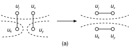
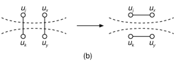
Figure 2: The two possibilities for an edge switch to produce an unconnected graph. In part (a), $(u_{j},u_{k})$ and $(u_{x},u_{y})$ constitute a nonadjacent, non-neighbor bridge pair. In part (b), $(u_{j},u_{k})$ and $(u_{x},u_{y})$ constitute a nonadjacent, non-neighbor pair cut. The dashed lines delimit the connected components that appear when the edges crossing them are removed from the graph.

Clearly, there are $\binom{m}{2}=m(m-1)/2$ pairs of distinct edges, and on each one we may perform up to two edge switches, depending on how many are feasible. Let $\mu^{\mathrm{b}}_{i}$ be the ratio of the number of nonadjacent, non-neighbor bridge pairs in $G_{i}$ to $m(m-1)$. Note that $\mu^{\mathrm{b}}_{i}$ gives the probability that we choose a nonadjacent, non-neighbor bridge pair and perform on it the edge switch that produces an unconnected graph. Likewise, let $\mu^{\mathrm{c}}_{i}$ be the ratio of the number of nonadjacent, non-neighbor pair cuts in $G_{i}$ to $m(m-1)$. Then $\mu^{\mathrm{c}}_{i}$ is the probability that we choose a nonadjacent, non-neighbor pair cut and perform on it the edge switch that produces an unconnected graph. We clearly have

$$\rho_{i}=1-\mu^{\mathrm{b}}_{i}-\mu^{\mathrm{c}}_{i}.$$ (3)

In Appendix A we give a connectivity test that calculates the value of $\rho_{i}$ and is asymptotically no harder than depth-first search in the worst case.

If $G_{i}$ is the graph obtained right after a connectivity test, then the intuition behind the SB heuristic indicates that $w$ should be adjusted in a way that led to $\alpha=(\rho_{i})^{w}$, yielding

$$w=\frac{\ln\alpha}{\ln\rho_{i}}.$$ (4)

Notice, however, that each graph $G_{i}$ of ${\cal G}_{D}$ may have a different $\rho_{i}$, so the Markov chain modeling this method might converge to a stationary distribution that is different from the uniform distribution. For this reason, we define $\bar{\rho}(t)$ to be the average of every $\rho_{i}$ obtained right after each of the first $t+1$ connectivity tests (the initial one and the $t$ others that correspond to transitions). We then let the SB heuristic adjust $w$ according to

$$w=\left\lceil\frac{\ln\alpha}{\ln\bar{\rho}(t)}\right\rceil$$ (5)

right after the $t$th connectivity test. Note, in connection with (5), that $w$ is assuredly a positive integer. Furthermore, for the reasons discussed in Section 3.1, we limit $w$ by a fixed upper bound $W$.

We remark, finally, that as a consequence of $w$ being adjusted as a function of every $\rho_{i}$ ever obtained, the method cannot be modeled as a Markov chain and, to be rigorous, can no longer even be treated as a variation of the ESMC method in which another heuristic is used. However, if $\bar{\rho}(t)$ converges as $t\to\infty$, then $w$ also converges. In this case, $w$ approaches a constant and, as noted in Section 2, we once again have a method that can be modeled as a Markov chain having a uniform stationary distribution. In Section 4, our approach to assessing the convergence of $\bar{\rho}(t)$ (and of $w$, consequently) is to compare the average value of $g(t)$ at the end of an execution under the SB heuristic to those obtained under the GMZ and VL heuristics. As we demonstrate in that section, the figures for the SB heuristic vary within relatively small percentages with respect to those of either of the other two heuristics and we take this as indication that $\bar{\rho}(t)$ is close to convergence. In what follows, then, we continue to refer to the SB heuristic as an alternative for use with the ESMC method.

4 Computational results

In this section we present computational results for the three heuristics of Section 3. We have concentrated on power laws with $\tau=2.0,2.1,\ldots,3.0$ and set $n=10^{3}$. All experiments were carried out on a Pentium 4HT running at 3GHz with 1GB of main memory. All running times we report refer to total elapsed times under a Linux operating system hosting one single user.

Before discussing our experiments, we pause momentarily to elaborate on a curious behavior of the power-law distribution. From Section 1, we know that, in order for $D$ to be realizable, its average node degree must be no less than the average node degree of a tree, which is approximately $2$ for sufficiently large $n$. For $n=10^{3}$, this is expected to hold only for $\tau\lessapprox 2.47$, meaning that for $\tau\gtrapprox 2.47$ $D$ is expected not to be realizable. By requiring realizability as we repeatedly sample $D$ from the power law, we are in fact making the node-degree distribution be slightly different from that very power law. What we have observed is that, for $\tau\gtrapprox 2.47$, the node-degree variance for realizable degree sequences tends to increase with $\tau$ while the number of edges remains roughly constant. These characteristics have affected the results we present next very strongly.

In our experiments, we used $W=10^{4}$. For each value of $\tau$, we sampled $600$ realizable degree sequences and, for each of them, executed the generation method using the three heuristics and two distinct halting conditions. We carried out the VL heuristic for $q^{+}=0.1,0.2,0.3$ and set $q^{-}$ in such a way that $q^{+}/q^{-}=e-1$. The SB heuristic was carried out for $\alpha=0.1,0.2,0.3$.

We have focused on analyzing four indicators, each calculated from the $600$ executions with each heuristic and each halting condition. The first one, which we denote by $R_{\mathrm{conv}}$, is the ratio of the average $g(t)$ value at the end of an execution to the average value of $\bar{g}(t)$ also at the end of an execution. $R_{\mathrm{conv}}$ can be used as a source of information on the convergence of the Markov chain, as we know that $\bar{g}(t)$ is an unbiased estimator for $g(t)$. Generally, the deviation of $R_{\mathrm{conv}}$ from $1$ grows with how far the generated graph is from a uniformly random sample of ${\cal G}_{D}$. The second indicator, which we denote by $R_{\mathrm{switch}}$, is the average number of edge switches performed during an execution that are not undone as a result of the connectivity test. The third indicator, which we denote by $R_{w}$, is the average value of $w$ at the end of an execution. The last indicator, finally, is the average running time (in minutes) of an execution and is denoted by $R_{\mathrm{time}}$.

4.1 Halting on the clustering coefficient

For the first halting condition, we have let $g(t)$ be the clustering coefficient of $G$. This coefficient is the ratio of three times the number of triangles in $G$ to the number of three-edge paths in $G$ (each triangle corresponds to three such paths) [24]. Calculating the clustering coefficient requires $O(d_{1}m)$ time, as a triangle is identified by checking whether an edge’s end nodes have a common neighbor. We have used $\delta=60$ and $\gamma=10^{-4}$ for this halting condition.

With regard to our discussion at the end of Section 3.2 on the convergence of $\bar{\rho}(t)$, we have observed the average value of $g(t)$ under the SB heuristic to vary within only roughly $5\%$ of the values obtained for the GMZ heuristic for most values of $\tau$, the exceptions being $\tau=2.4$ ($7.8\%$) and $\tau=2.5$ ($6.3\%$). As for the VL heuristic, the percentage drops to roughly $3\%$, the exceptions being the same with $5.7\%$ for $\tau=2.4$ and $5\%$ for $\tau=2.5$.

Figure 3 shows the results obtained with this halting condition for the GMZ heuristic (parts (a–d)), the VL heuristic (e–h), and the SB heuristic (i–l). The plots for $R_{\mathrm{conv}}$ (Figure 3(a, e, i)) show that $R_{\mathrm{conv}}$ is close to $1$ for all the three heuristics, especially when $\tau\leq 2.1$ or $\tau\geq 2.8$. The plots for $R_{\mathrm{switch}}$ (Figure 3(b, f, j)) show that the smallest value of $R_{\mathrm{switch}}$ is obtained for $\tau\approx 2.4$, suggesting that the clustering coefficient converges faster for such a value of $\tau$. The parameters $q^{+}$ and $q^{-}$ of the VL heuristic and $\alpha$ of the SB heuristic seem, curiously, to have small impact on $R_{\mathrm{switch}}$. Furthermore, since $m$ is almost constant for $\tau\geq 2.5$, $R_{\mathrm{switch}}$ does not seem to be proportional to $m$, as assumed in the analysis conducted in [29] for a slightly different power law. The plots for $R_{w}$ (Figure 3(c, g, k)) show that the smallest value of $R_{w}$ is also obtained when $\tau\approx 2.4$, indicating that the probability that an edge-switching attempt results in an unconnected $G$ is smaller when $\tau\approx 2.4$. We note that the highest $R_{w}$ is obtained with the SB heuristic. The reason for this behavior seems to be that both the GMZ heuristic and the VL heuristic start with $w=1$, while the SB heuristic starts with $w$ relatively close to $R_{w}$. The plots for $R_{\mathrm{time}}$ (Figure 3(d, h, l)) show that the SB heuristic yields on average the smallest running time, despite employing a more complex connectivity test. For example, the SB heuristic has on average outperformed the GMZ heuristic by roughly $12\%$ when $\tau=2.0$, $44\%$ when $\tau=2.3$, $61\%$ when $\tau=2.6$, and $74\%$ when $\tau=3.0$. In comparison to the VL heuristic, these figures have been roughly $21\%$ when $\tau=2.0$, $25\%$ when $\tau=2.3$, $51\%$ when $\tau=2.6$, and $56\%$ when $\tau=3.0$. Regarding the value of $\alpha$, the smallest average $R_{\mathrm{time}}$ for the SB heuristic corresponds to $\alpha=0.1$. We expect $R_{\mathrm{time}}$ to decrease even more if we continue decreasing $\alpha$, but this decrease will probably be progressively smaller until an optimal value of $\alpha$ is achieved. Also, it is curious to note that, for $\tau$ near $3.0$, the GMZ heuristic yields the smallest $R_{\mathrm{switch}}$ but the highest $R_{\mathrm{time}}$ in comparison to the other heuristics. In this situation, $R_{w}$ is so small that, even performing substantially fewer edge switches, the ESMC method requires on average much longer to conclude.

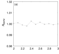
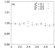
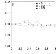
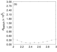
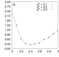
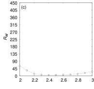
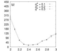
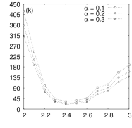
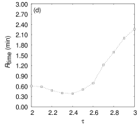
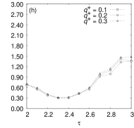
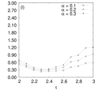
Figure 3: Computational results for the GMZ heuristic (a–d), the VL heuristic (e–h), and the SB heuristic (i–l) when the halting condition is based on the clustering coefficient. Plots refer to $R_{\mathrm{conv}}$ (a, e, i), $R_{\mathrm{switch}}$ (b, f, j), $R_{w}$ (c, g, k), and $R_{\mathrm{time}}$ (d, h, l).

Figure 4(a) presents the average $\mu^{\mathrm{b}}_{i}$ at the end of an execution for the SB heuristic when the halting condition is based on the clustering coefficient. The value of $\tau$ for which we obtain the highest average is $2.4$, in accordance with the fact that $R_{w}$ is on average minimum for this same value (cf. Figure 3(c, g, k)). When $\tau$ is decreased from $2.4$, on average $\mu^{\mathrm{b}}_{i}$ decreases as well, since the graph is expected to have more edges and, consequently, fewer bridges. When $\tau$ is increased from $2.4$, on average $\mu^{\mathrm{b}}_{i}$ also decreases. The reason in this case is that, since the number of edges remains practically constant as $\tau$ is increased from $2.4$, and moreover the variance within the degree sequence increases, the graph tends to acquire several star-like subgraphs and therefore the fraction of adjacent or neighbor bridge pairs is expected to increase. Figure 4(b) refers to $\mu^{\mathrm{c}}_{i}$. The behavior is similar, albeit in an extremely smaller scale, thus indicating that the fraction of nonadjacent, non-neighbor pair cuts in graphs whose node degrees are power-law-distributed is on average negligible. If we ignore pair cuts and use $\rho_{i}=1-\mu^{\mathrm{b}}_{i}$ in lieu of (3), then we obtain figures for $R_{\mathrm{time}}$ as shown in Figure 4(c). In this case $R_{\mathrm{time}}$ is on average significantly smaller than when pair cuts are not ignored (Figure 3(l)). This decrease is on average higher when $d_{1}$ is expected to be smaller. Since for small $d_{1}$ the time complexity of calculating the clustering coefficient is relatively close to the time complexity of a connectivity test, speeding-up the connectivity test impacts more strongly the overall running time. For example, when $\tau=2.4$, in which case we have observed the value of $d_{1}$ to be relatively small on average, ignoring pair cuts leads to a decrease in $R_{\mathrm{time}}$ of about $31\%$ on average. Likewise, when $\tau=2.0$, in which case we have observed the opposite trend regarding the value of $d_{1}$, the decrease in $R_{\mathrm{time}}$ is of about $7\%$.

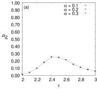
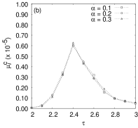
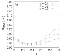
Figure 4: Plots for $\mu^{\mathrm{b}}_{i}$ (a), $\mu^{\mathrm{c}}_{i}$ (b), and $R_{\mathrm{time}}$ when pair cuts are ignored (c). The halting condition is the one based on the clustering coefficient.

4.2 Halting on the average distance between nodes

The second halting condition is based on letting $g(t)$ be the average distance between the nodes of $G$, which can be calculated by conducting a breath-first search rooted at each node of $G$. This calculation requires $\Theta(nm)$ time, therefore more than the calculation of the clustering coefficient. We have used $\delta=30$ and $\gamma=10^{-3}$ for this halting condition.

As we once again return to the issue raised at the end of Section 3.2 on the convergence of $\bar{\rho}(t)$, for this second halting condition we have observed the average value of $g(t)$ under the SB heuristic to stay below roughly $1\%$ of the values obtained for the GMZ heuristic for all values of $\tau$. As for the VL heuristic, the percentage remains the same but for $\tau=2.1$ ($1.8\%$).

Figure 5 shows the results when this is the halting condition for the GMZ heuristic (parts (a–d)), the VL heuristic (e–h), and the SB heuristic (i–l). The plots for $R_{\mathrm{conv}}$ (Figure 5(a, e, i)) show that $R_{\mathrm{conv}}$ is relatively far from $1$ in comparison to the results obtained with the first halting condition (Figure 3(a, e, i)). In order to obtain $R_{\mathrm{conv}}$ closer to $1$, we may need to increase $\delta$ and/or decrease $\gamma$. Despite being not so close to $1$, the value of $R_{\mathrm{conv}}$ is almost the same regardless of which heuristic is used to adjust $w$. The plots for $R_{\mathrm{switch}}$ (Figure 5(b, f, j)) show that the smallest value of $R_{\mathrm{switch}}$ occurs when $\tau\approx 2.4$. Similarly to the case of the clustering coefficient, this suggests that the average distance between nodes converges faster when $\tau\approx 2.4$. The plots for $R_{w}$ (Figure 5(c, g, k)) also show that the smallest $R_{w}$ is obtained for $\tau\approx 2.4$. Regarding $R_{\mathrm{time}}$ (Figure 5(d, h, l)), the plots show that the SB heuristic leads once again to the smallest running time on average. For example, on average the SB heuristic outperforms the GMZ heuristic by roughly $77\%$ when $\tau=2.0$, $86\%$ when $\tau=2.3$, $85\%$ when $\tau=2.6$, and $75\%$ when $\tau=3.0$. In comparison to the VL heuristic, on average the SB heuristic outperforms it by roughly $41\%$ when $\tau=2.0$, $80\%$ when $\tau=2.3$, $82\%$ when $\tau=2.6$, and $54\%$ when $\tau=3.0$. The average gain obtained with the SB heuristic is higher under this halting condition, which can be explained by noting that each transition is now slower than under the halting condition based on the clustering coefficient. As a consequence, it is under the average-distance halting condition that the impact of adjusting $w$ properly is more strongly manifest. Also, and unlike what occurs with the first halting condition, the gain obtained with the SB heuristic is now higher when $\tau$ is around $2.4$. This suggests that the choice for $g(t)$ depends on a careful consideration of each application’s peculiarities. Regarding the value of $\alpha$, the SB heuristic once again leads to the smallest $R_{\mathrm{time}}$ when $\alpha=0.1$, suggesting that the optimal value of $\alpha$ is less than $0.1$.

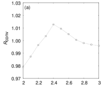
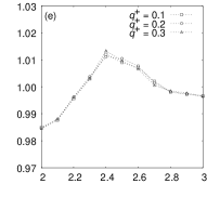
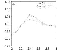
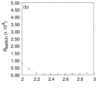
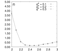
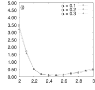
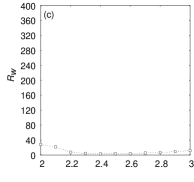
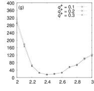
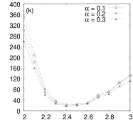
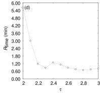
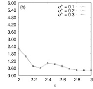
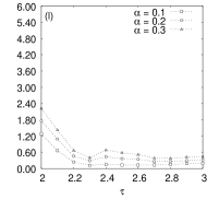
Figure 5: Computational results for the GMZ heuristic (a–d), the VL heuristic (e–h), and the SB heuristic (i–l) when the halting condition is based on the average distance between nodes. Plots refer to $R_{\mathrm{conv}}$ (a, e, i), $R_{\mathrm{switch}}$ (b, f, j), $R_{w}$ (c, g, k), and $R_{\mathrm{time}}$ (d, h, l).

Figure 6 presents, respectively in parts (a) and (b), the average $\mu^{\mathrm{b}}_{i}$ and $\mu^{\mathrm{c}}_{i}$ for the SB heuristic when the halting condition is based on the average distance between nodes. The results are similar to the ones shown in Figure 4(a, b) for the halting condition based on the clustering coefficient. The plots for $R_{\mathrm{time}}$ (Figure 6(c)), on the other hand, show a very different behavior. For almost all values of $\tau$, $R_{\mathrm{time}}$ is now seen to increase slightly when pair cuts are ignored. The reason for this behavior seems to be an insufficient number of samples. In fact, we expect $R_{\mathrm{time}}$ to be very slightly smaller than that obtained when pair cuts are not ignored. Since the time complexity of calculating the average distance between nodes is significantly higher than that of a connectivity test, ignoring pair cuts is therefore expected to have a small impact on the overall running time of the method.

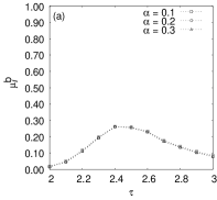
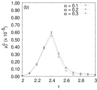
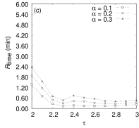
Figure 6: Plots for $\mu^{\mathrm{b}}_{i}$ (a), $\mu^{\mathrm{c}}_{i}$ (b), and $R_{\mathrm{time}}$ when pair cuts are ignored (c). The halting condition is the one based on the average distance between nodes.

5 Conclusions

We have considered the problem of generating, uniformly at random, connected graphs that have a given degree sequence but no multiple edges or self-loops. We studied the ESMC method, which employs edge switches to transform a graph into another while preserving the degree sequence. This method consists of first deterministically finding a graph with the desired properties and then performing random edge switches and also connectivity tests to obtain a randomized result.

We showed that, if we attempt to perform a constant number $w$ of edge switches between successive connectivity tests, then the method can be modeled as a Markov chain having a uniform stationary distribution. We also showed that, if $w$ is not constant but rather is adjusted as a function of the last connectivity test’s outcome, then the method can still be modeled as a Markov chain of uniform stationary distribution.

We have also introduced a new heuristic for adjusting $w$ that depends on the probability that the graph being generated remains connected after an edge switch is attempted. In order to calculate this probability, we use a new connectivity test that has the same time and space complexities as depth-first search (cf. Appendix A). Even though the resulting method cannot always be modeled as a Markov chain, we showed that there are circumstances under which it too converges to the uniform distribution.

One of the main issues regarding generation methods based on Markov chains is determining the number of transitions to be performed until the Markov chain is satisfactorily close to its stationary distribution. We have approached this issue by resorting to the pragmatic procedure of computing, after each transition, a certain function of the graph being generated, and halting the generation when the average of this function over all transitions seems to have converged. A proper choice for this function is essential to the efficacy of the method, but appears to require consideration on a case-by-case basis.

We have given computational results for power-law-based degree sequences. Our results contemplate two previous heuristics for adjusting $w$ and also our new heuristic, and were given for two distinct halting criteria. They show that our heuristic, on average, outperforms the two existing heuristics on power laws for which $2\leq\tau\leq 3$.

The ESMC method can be especially useful to generate a group of connected random graphs having the same degree sequence. After obtaining the first graph, we can continue performing a relatively small number of transitions to generate each additional instance, without having to run the method from its beginning. Finally, the ESMC method can be extended to generate random graphs having a given degree sequence and another desired property (e.g., graphs having the clustering coefficient limited to a given interval). We need only find a means of obtaining an initial graph having that property, then obtain an efficient procedure to test whether a graph has that property, and also show the irreducibility of the Markov chain, that is, show that there is a sequence of edge-switching attempts connecting any two graphs having the given degree sequence and the desired property.

Acknowledgments

The authors acknowledge partial support from CNPq, CAPES, and a FAPERJ BBP grant.

Appendix A The new connectivity test

Given a graph $G_{i}$ of ${\cal G}_{D}$, we show how a modified depth-first search on $G_{i}$ can be used to obtain $\rho_{i}$ in addition to testing whether $G_{i}$ is connected. Let $S_{i}$ be the directed graph induced by a depth-first search on $G_{i}$. This graph contains the same nodes as $G_{i}$ and a directed edge for each edge of $G_{i}$. The direction of an edge in $S_{i}$ is the direction along which the search traverses the edge for the first time. Let $(u_{j}\to u_{k})$ be an edge of $S_{i}$. We say that $u_{j}$ is the parent of $u_{k}$ (or, equivalently, $u_{k}$ is a child of $u_{j}$) if the search visits $u_{k}$ for the first time from $u_{j}$. Edge $(u_{j}\to u_{k})$ is then called a tree edge, as it is part of a directed spanning tree rooted at the start node of the search. If the search does not visit $u_{k}$ for the first time from $u_{j}$, then $(u_{j}\to u_{k})$ is called a back edge, as it necessarily represents a move toward an already visited node. Figure 7 shows an example $S_{i}$; nodes are numbered in such a way that an edge is a tree edge if and only if it leads from a lower-numbered node to a higher-numbered one.

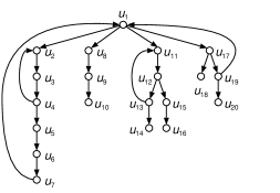
Figure 7: An example $S_{i}$. Nodes are visited in the order $u_{1},\ldots,u_{20}$.

The level of a node $u_{j}$ in $S_{i}$ is the length of the shortest directed path from the root to $u_{j}$. The descent and ancestry of $u_{j}$ in $S_{i}$ are, respectively, the set of nodes toward which a tree path exists from $u_{j}$ and the set of nodes from which a tree path exists toward $u_{j}$. Node $u_{j}$ is excluded from either set. Let $(u_{j}\to u_{k})$ be a tree edge and $(u_{x}\to u_{y})$ a back edge. We say that $(u_{x}\to u_{y})$ covers $(u_{j}\to u_{k})$ if $u_{x}=u_{k}$ or $u_{x}$ belongs to the descent of $u_{k}$, and furthermore $u_{y}=u_{j}$ or $u_{y}$ belongs to the ancestry of $u_{j}$. In Figure 7, edge $(u_{4}\to u_{2})$ covers edges $(u_{2}\to u_{3})$ and $(u_{3}\to u_{4})$.

Let us proceed to the calculation of $\rho_{i}$, which by (3) depends on $\mu^{\mathrm{b}}_{i}$ and $\mu^{\mathrm{c}}_{i}$.

A.1 Handling bridge pairs

Clearly, the number of nonadjacent, non-neighbor bridge pairs of $G_{i}$, on which $\mu^{\mathrm{b}}_{i}$ is based, can be obtained from the number of bridges of $G_{i}$, the number of pairs of adjacent bridges of $G_{i}$, and the number of neighbor bridge pairs of $G_{i}$. During the search, we count some undirected paths in $S_{i}$ (i.e., paths whose edges’ directions are ignored) having certain special properties. For each node $u_{j}$, we use the counters $B^{\mathrm{b}}_{j}$, $B^{\mathrm{bb}}_{j}$, $B^{\mathrm{bbb}}_{j}$, $B^{\mathrm{nb}}_{j}$, and $B^{\mathrm{bnb}}_{j}$ to record how many undirected paths of $S_{i}$ start at $u_{j}$, proceed through nodes in the descent of $u_{j}$ exclusively, and moreover consist in $G_{i}$ of, respectively, one bridge, two bridges, three bridges, a non-bridge edge followed by a bridge, and two bridges separated by a non-bridge edge. We now explain how these counters can be used to obtain the number of nonadjacent, non-neighbor bridge pairs of $G_{i}$ and also how we can calculate them during the search.

The number of bridges of $G_{i}$ can be easily obtained during the search, as an edge of $G_{i}$ is a bridge if and only if it is a tree edge of $S_{i}$ that is not covered by any back edge (e.g., $(u_{1}\to u_{8})$ in Figure 7). What we do is simply to accumulate $B^{\mathrm{b}}_{j}$ into a global counter as the exploration of $u_{j}$ concludes. Obtaining the number of pairs of adjacent bridges of $G_{i}$ is also simple, since it is a matter of accumulating, as the exploration of $u_{j}$ concludes, the number of pairs of adjacent bridges that are incident to $u_{j}$ and its descendants, that is,

$$\binom{B^{\mathrm{b}}_{j}}{2}+B^{\mathrm{bb}}_{j}.$$ (6)

As for obtaining the number of neighbor bridge pairs, note first that the edge connecting the two bridges can be of three types. It can be another bridge (e.g., $(u_{1}\to u_{8})$ connecting $(u_{1}\to u_{11})$ to $(u_{8}\to u_{9})$, and $(u_{8}\to u_{9})$ connecting $(u_{1}\to u_{8})$ to $(u_{9}\to u_{10})$ in Figure 7); it can be a tree edge that is not a bridge (e.g., $(u_{1}\to u_{17})$ connecting $(u_{1}\to u_{11})$ to $(u_{17}\to u_{18})$, and $(u_{11}\to u_{12})$ connecting $(u_{1}\to u_{11})$ to $(u_{12}\to u_{15})$ in Figure 7); and, finally, it can be a back edge (e.g., $(u_{19}\to u_{1})$ connecting $(u_{1}\to u_{11})$ to $(u_{19}\to u_{20})$, and $(u_{13}\to u_{11})$ connecting $(u_{1}\to u_{11})$ to $(u_{13}\to u_{14})$ in Figure 7). Let then $(u_{j}\to u_{k})$ be a tree edge. As the exploration of $u_{k}$ concludes, for each $u_{x}$ in $u_{k}$’s descent from which a back edge exists toward $u_{k}$, we add $B^{\mathrm{b}}_{x}$ to $B^{\mathrm{nb}}_{k}$. We then accumulate

$$B^{\mathrm{bb}}_{k}(B^{\mathrm{b}}_{k}-1)+B^{\mathrm{bbb}}_{k}+B^{\mathrm{b}}_{k}B^{\mathrm{nb}}_{k}+B^{\mathrm{bnb}}_{k}$$ (7)

into the global counter of neighbor bridge pair of $G_{i}$. When at last the search returns to $u_{k}$’s parent $u_{j}$, we do one of the following: if $(u_{j}\to u_{k})$ is a bridge, then we increment $B^{\mathrm{b}}_{j}$ and add $B^{\mathrm{b}}_{k}$ to $B^{\mathrm{bb}}_{j}$, $B^{\mathrm{bb}}_{k}$ to $B^{\mathrm{bbb}}_{j}$, and $B^{\mathrm{nb}}_{k}$ to $B^{\mathrm{bnb}}_{j}$; otherwise, we add $B^{\mathrm{b}}_{k}$ to $B^{\mathrm{nb}}_{j}$.

A.2 Handling pair cuts

The number of nonadjacent, non-neighbor pair cuts, which is the basis for computing $\mu^{\mathrm{c}}_{i}$, can be obtained by calculating the number of pair cuts, the number of adjacent pair cuts, and the number of neighbor pair cuts. Two edges of $S_{i}$ form a pair cut if and only if they are covered by one single common back edge (e.g., $(u_{1}\to u_{2})$ and $(u_{4}\to u_{5})$ in Figure 7). In order to identify pair cuts during the search, for each node we store the back edge that connects either the node itself or one of its descendants to its lowest-level ancestor. If more than one back edge reaches the same node, then we need store neither, since no edge through which the search is yet to backtrack can be uniquely covered by any of them.

Let $(u_{j}\to u_{k})$ be a tree edge. Assume that $(u_{j}\to u_{k})$ is covered only by the edge $(u_{x}\to u_{y})$ and let $C_{(u_{x}\to u_{y})}$ be a counter of the number of edges covered only by $(u_{x}\to u_{y})$. Clearly, the number of pair cuts either covered by $(u_{x}\to u_{y})$ or including this edge is $\binom{C_{(u_{x}\to u_{y})}+1}{2}$, since $(u_{x}\to u_{y})$ also participates in a pair cut along with each of the $C_{(u_{x}\to u_{y})}$ edges that it covers. This number is accumulated into a global counter of the pair cuts of $G_{i}$ as the search detects that no edge through which it is yet to backtrack is covered only by $(u_{x}\to u_{y})$.

In order to identify adjacent and neighbor pair cuts, we need to keep some information regarding $(u_{x}\to u_{y})$ and the edges covered only by it as the search backtracks from $u_{k}$. Besides $(u_{x}\to u_{y})$ itself and $C_{(u_{x}\to u_{y})}$, we also need to retain information on three other nodes, which we denote by $v_{1}$, $v_{2}$, and $v_{3}$. Nodes $v_{1}$ and $v_{2}$ are the two lowest-level nodes such that the edge between each of them and its parent is covered only by $(u_{x}\to u_{y})$. Node $v_{3}$ is the highest-level node such that the edge between it and its parent is covered only by $(u_{x}\to u_{y})$. For example, as the search backtracks from $u_{3}$ in the case of Figure 7, we store the back edge $(u_{7}\to u_{1})$ and let $v_{1}=u_{5}$, $v_{2}=u_{6}$, and $v_{3}=u_{7}$.

Assume now that the search has concluded the exploration of all the neighbors of $u_{j}$. In the case of a child $u_{k}$ of $u_{j}$, assume as above that $(u_{j}\to u_{k})$ is covered only by the back edge $(u_{x}\to u_{y})$. Adjacent pair cuts can be identified in three scenarios: when $u_{k}=u_{x}$ (Figure 8(a)), when $u_{j}=u_{y}$ (Figure 8(b)), and when $u_{k}$ is the parent of $v_{1}$ (Figure 8(c)). As for neighbor pair cuts, there are five cases. The first case happens when a tree edge connects $(u_{x}\to u_{y})$ to one of the tree edges covered only by it; this can be identified either when $u_{x}$ is a child of $u_{k}$ (Figure 8(d)) or when $u_{y}$ is the parent of $u_{j}$ (Figure 8(e)). The second case occurs when another back edge connects $(u_{x}\to u_{y})$ to one of the tree edges covered only by it; this can be identified either by the existence of the back edge $(u_{x}\to u_{k})$ (Figure 8(f)) or by the existence of the back edge $(u_{j}\to u_{y})$ (Figure 8(g)). The third case occurs when $(u_{x}\to u_{y})$ connects two edges covered only by it, and can be identified when $u_{j}=u_{y}$ and $u_{x}=v_{3}$ (Figure 8(h)). The fourth case occurs when a tree edge connects two other tree edges, the latter two covered only by $(u_{x}\to u_{y})$; this case can be identified by $v_{1}$ or $v_{2}$ being two levels above $u_{k}$ (Figure 8(i)). The fifth and last case happens when another back edge connects two edges covered only by $(u_{x}\to u_{y})$, which can be identified by the existence of a back edge from the parent of $v_{1}$ to $u_{k}$ (Figure 8(j)). After updating the number of adjacent pair cuts and neighbor pair cuts before the search backtracks from $u_{j}$, we increment $C_{(u_{x}\to u_{y})}$ and let $v_{2}=v_{1}$ and $v_{1}=u_{k}$. If no node is currently marked as $v_{3}$, then we also let $v_{3}=u_{k}$.

Figure 8: Scenarios for the occurrence of adjacent and neighbor pair cuts.

A.3 Complexity

Let us now discuss the space and time complexities of this modified depth-first search. Clearly, the ESMC method requires $\Omega(m)$ space, since we need to store an array with the edges of the graph being generated. During the search, for each node $u_{k}$, we need to store its parent (say, $u_{j}$), its level, the $B^{\mathrm{}}_{k}$’s, and the back edge covering $(u_{j}\to u_{k})$ that reaches the lowest-level node. If $(u_{x}\to u_{y})$ is this edge, then we also need to store the $v_{1}$, $v_{2}$, $v_{3}$, and $C_{(u_{x}\to u_{y})}$ corresponding to $(u_{j}\to u_{k})$. Summing up over all nodes, this information requires only $\Theta(n)$ space. Furthermore, for each node we keep a list of the back edges arriving at it for the sake of handling the cases in Figure 8(f, j), which requires $O(m)$ space overall. We also, finally, keep a global $n$-element array for nodes to register the back edges originating at them. This is needed for identifying the occurrence of the scenario illustrated in Figure 8(g). We then see, in summary, that the modified depth-first search does not change the space complexity of the ESMC method.

Obtaining the time complexity requires that we detail the steps performed during the exploration of a node $u_{j}$ of $G_{i}$. First we explore each neighbor $u_{k}$ of $u_{j}$, and update the $B^{\mathrm{}}_{j}$’s if $(u_{j}\to u_{k})$ is a tree edge. Otherwise, if $(u_{j}\to u_{k})$ is a back edge, then we include it in the list of back edges arriving at $u_{k}$ and record the back edge that leaves $u_{j}$ and arrives at its lowest-level ancestor. After exploring the entire descent of $u_{j}$, for each node toward which there is a back edge leaving $u_{j}$ we set a mark in the $n$-element array. Then, for each child $u_{k}$ of $u_{j}$, we update the counters of pair cuts using the $n$-element array, the information regarding the back edge, say $(u_{x}\to u_{y})$, that reaches the lowest-level node, and the list of back edges arriving at $u_{k}$. The edge $(u_{x}\to u_{y})$ may become the back edge that arrives at $u_{j}$’s lowest-level ancestor; in this case, we also update $C_{(u_{x}\to u_{y})}$, $v_{1}$, $v_{2}$, and $v_{3}$, which requires $O(1)$ time. We then reset all marks in the $n$-element array, and for each back edge arriving at $u_{j}$ we update $B^{\mathrm{nb}}_{j}$, which also requires only $O(1)$ time for each edge. Finally, we conclude the exploration of $u_{j}$ by updating the counters of adjacent and neighbor bridge pairs using (6) and (7). We then see that a tree edge $(u_{j}\to u_{k})$ is visited at most three times, twice when $u_{j}$ and $u_{k}$ are exploring their neighbors, and once more when $u_{j}$ revisits the tree edges leaving it to update the pair-cut counters and the back edge reaching the lowest-level node. Each back edge $(u_{x}\to u_{y})$, in turn, is visited at most six times, twice when $u_{x}$ and $u_{y}$ are exploring their neighbors, twice when $u_{x}$ set and reset marks in the $n$-element array, once when updating $B^{\mathrm{nb}}_{y}$, and once more when the parent of $u_{y}$ is updating the number of neighbor pair cuts (cf. the cases illustrated in Figure 8(f, j)). In conclusion, the time complexity of the modified depth-first search is $O(m)$, thus the same as that of the standard depth-first search.

References

- [1] D. Achlioptas, A. Clauset, D. Kempe, and C. Moore. On the bias of traceroute sampling: or, power-law degree distributions in regular graphs. In Proceedings of the Thirty-Seventh Annual ACM Symposium on Theory of Computing, pages 694–703, 2005.
- [2] L. A. Adamic, R. M. Lukose, and B. A. Huberman. Local search in unstructured networks. In S. Bornholdt and H. G. Schuster, editors, Handbook of Graphs and Networks: From the Genome to the Internet, pages 295–317. Wiley-VCH, Weinheim, Germany, 2003.
- [3] R. Albert and A.-L. Barabási. Statistical mechanics of complex networks. Reviews of Modern Physics, 74:47–97, 2002.
- [4] R. Albert, H. Jeong, and A.-L. Barabási. Error and attack tolerance of complex networks. Nature, 406:378–382, 2000.
- [5] R. P. Anstee. An algorithmic proof of Tutte’s -factor theorem. Journal of Algorithms, 6:112–131, 1985.
- [6] A.-L. Barabási and R. Albert. Emergence of scaling in random networks. Science, 286:509–512, 1999.
- [7] C. Berge. Graphs. North-Holland, Amsterdam, The Netherlands, 1989.
- [8] B. Bollobás. Random Graphs. Cambridge University Press, Cambridge, UK, second edition, 2001.
- [9] B. Bollobás and O. Riordan. Mathematical results on scale-free random graphs. In S. Bornholdt and H. G. Schuster, editors, Handbook of Graphs and Networks: From the Genome to the Internet, pages 1–34. Wiley-VCH, Weinheim, Germany, 2003.
- [10] R. Cohen, K. Erez, D. ben-Avraham, and S. Havlin. Resilience of the Internet to random breakdowns. Physical Review Letters, 85:4626–4628, 2000.
- [11] P. Erdős and T. Gallai. Graphs with prescribed degrees of vertices. Matematikaies Fizikai Lapok, 11:264–274, 1960.
- [12] P. Erdős and A. Rényi. On random graphs. Publicationes Mathematicae, 6:290–297, 1959.
- [13] M. Faloutsos, P. Faloutsos, and C. Faloutsos. On power-law relationships of the Internet topology. In Proceedings of the Conference on Applications, Technologies, Architectures, and Protocols for Computer Communication, pages 251–262, 1999.
- [14] H. N. Gabow. An efficient reduction technique for degree-constrained subgraph and bidirected network flow problems. In Proceedings of the Fifteenth Annual ACM Symposium on Theory of Computing, pages 448–456, 1983.
- [15] C. Gkantsidis, M. Mihail, and A. Saberi. Hybrid search schemes for unstructured peer-to-peer networks. In Proceedings of the Conference on Computer Communications, pages 1526–1537, 2005.
- [16] C. Gkantsidis, M. Mihail, and E. Zegura. The Markov chain simulation method for generating connected power law random graphs. In Proceedings of the Fifth Workshop on Algorithm Engineering and Experiments, 2003.
- [17] S. Hakimi. On the realizability of a set of integers as degrees of the vertices of a graph. SIAM Journal on Applied Mathematics, 10:496–506, 1962.
- [18] V. Havel. A remark on the existence of finite graphs. Časopis pro Pěstování Matematiky, 80:477–480, 1955.
- [19] M. Jerrum, A. Sinclair, and E. Vigoda. A polynomial-time approximation algorithm for the permanent of a matrix with non-negative entries. Journal of the ACM, 51:671–697, 2004.
- [20] S. Karlin and H. M. Taylor. A First Course in Stochastic Processes. Academic Press, New York, NY, second edition, 1975.
- [21] J. H. Kim and V. H. Vu. Generating random regular graphs. In Proceedings of the Thirty-Fifth Annual ACM Symposium on Theory of Computing, pages 213–222, 2003.
- [22] A. Medina, I. Matta, and J. Byers. On the origin of power laws in Internet topologies. Computer Communication Review, 30(2):18–28, 2000.
- [23] M. Mitzenmacher and E. Upfal. Probability and Computing: Randomized Algorithms and Probabilistic Analysis. Cambridge University Press, New York, NY, 2005.
- [24] M. E. J. Newman. The structure and function of complex networks. SIAM Review, 45:167–256, 2003.
- [25] A. R. Rao, R. Jana, and S. Bandyopadhyay. A Markov chain Monte Carlo method for generating random -matrices with given marginals. The Indian Journal of Statistics, 58:225–242, 1996.
- [26] A. Sinclair. Algorithms for Random Generation and Counting: a Markov Chain Approach. Birkhäuser, Boston, MA, 1993.
- [27] H. Tangmunarunkit, R. Govindan, S. Jamin, S. Shenker, and W. Willinger. Network topology generators: degree-based vs. structural. In Proceedings of the Conference on Applications, Technologies, Architectures, and Protocols for Computer Communication, pages 147–159, 2002.
- [28] R. Taylor. Constrained switchings in graphs. Lecture Notes in Mathematics, 884:314–336, 1981.
- [29] F. Viger and M. Latapy. Efficient and simple generation of random simple connected graphs with prescribed degree sequence. Lecture Notes in Computer Science, 3595:440–449, 2005.