Rebounce and Black hole formation in a Gravitational Collapse Model with Vanishing Radial Pressure

Abstract

We examine spherical gravitational collapse of a matter model with vanishing radial pressure and non-zero tangential pressure. It is seen analytically that the collapsing cloud either forms a black hole or disperses depending on values of the initial parameters which are initial density, tangential pressure and velocity profile of the cloud. A threshold of black hole formation is observed near which a scaling relation is obtained for the mass of black hole, assuming initial profiles to be smooth. The similarities in the behaviour of this model at the onset of black hole formation with that of numerical critical behaviour in other collapse models are indicated.

I Introduction

Astrophysical black holes have a minimum mass, known as the Chandrashekhar mass. Realistic matter in a star is almost stationary at the initial epoch of its collapse and has a characteristic scale which depends on the properties of matter. If one does not restrict to stationary realistic matter, then in principle one should be able to produce arbitrary small mass black holes from initially collapsing cloud, as there will not be any characteristic scale present in the cloud and the positive pressure in the cloud has tendency to push the matter in radially outward direction in spherically symmetric situation.

There can be very many possible equation of states with pressure present that the collapsing matter can satisfy, but the non-linear Einstein equations are tractable analytically only for a very few equations of state. Here, we examine a spherically symmetric collapse model, in which the radial pressure vanishes and non-zero tangential pressure is present in the cloud. The Einstein cluster is such an example with vanishing radial pressure, where a cloud of rotating particles whose motion is sustained by an angular momentum has an average effect of creating a non-zero tangential stress. Such a static system was first introduced by Einstein ein , which was later generalized to non-static case Bondi . Subsequently, the gravitational collapse models with a vanishing radial pressure have been investigated extensively by Magli magli and others tan for the purpose of examining the validity or otherwise of the cosmic censorship conjectures and to understand the black hole and naked singularity formation in gravitational collapse.

We observe an intriguing feature in this model that it has a threshold of black hole formation and it shows a power law behaviour for the mass of the black hole near this threshold. We work in the comoving coordinates $(t,r,\theta,\phi)$ and construct an effective potential for the collapsing shells, with the aid of which one can see transparently the various possible evolutions of the collapsing shells. We demonstrate for a set of initial data that the collapsing cloud either forms a black hole or completely disperses, depending on the values of initial parameters. We point out similarities in behavior of this model at the threshold of black hole formation with already established critical behavior seen in other matter models radiation .

The outline of the paper is as follows. In Section II, we discuss the collapse equations and regularity conditions and in Section III, a tangential pressure model is constructed. In Section IV, various possible dynamical evolutions are illustrated and a scaling relation for the black hole mass is obtained. Discussion and conclusions are outlined in Section V.

II Einstein Equations, Regularity and Energy Conditions

We consider four dimensional spherically symmetric metric in comoving coordinates,

$$ds^{2}=-e^{2\nu(t,r)}dt^{2}+e^{2\psi(t,r)}dr^{2}+R^{2}(t,r)d\Omega^{2},$$ (1)

where $d\Omega^{2}$ is the line element on two-sphere. The energy-momentum tensor is then diagonal for any general Type I collapsing matter field and is given as $T^{t}_{t}=-\rho;\;T^{r}_{r}=p_{r};\;T^{\theta}_{\theta}=T^{\phi}_{\phi}=p_{\theta}$. This is a general class of matter fields that includes many known physical forms of matter he . The quantities $\rho$, $p_{r}$ and $p_{\theta}$ are the density, radial and tangential pressures respectively. We take the matter field to satisfy the weak energy condition, that is, the energy density measured by any local observer be non-negative. Then for any timelike vector $V^{i}$ we have $T_{ik}V^{i}V^{k}\geq 0$, i.e. $\rho\geq 0;\;\rho+p_{r}\geq 0;\;\rho+p_{\theta}\geq 0$. The dynamical evolution of the system is determined by the Einstein equations and for metric (1) these are given as

$$\rho=\frac{F^{\prime}}{R^{2}R^{\prime}},\;\;\;\;p_{r}=-\frac{\dot{F}}{R^{2}\dot{R}},$$ (2)

$$\nu^{\prime}(\rho+p_{r})=2(p_{\theta}-p_{r})\frac{R^{\prime}}{R}-p_{r}^{\prime},$$ (3)

$$-2\dot{R^{\prime}}+R^{\prime}\frac{\dot{G}}{G}+\dot{R}\frac{H^{\prime}}{H}=0,$$ (4)

$$G-H=1-\frac{F}{R},$$ (5)

where $(\,\dot{}\,)$ and $(^{\prime})$ are partial derivatives with respect to $t$ and $r$ respectively and

$$G(t,r)=e^{-2\psi}R^{\prime 2},\;\;H(t,r)=e^{-2\nu}\dot{R}^{2}.$$ (6)

The function $F(t,r)$ is twice the Misner-Sharp mass for the collapsing cloud, which gives the total mass within the shell of comoving radius $r$ at time $t$ misner . Regularity at the initial epoch implies $F(t_{i},0)=0$, that is, the mass function vanishes at the center of the cloud. It is seen from (2) that the density of matter blows up when $R=0$ or $R^{\prime}=0$. Here $R^{\prime}=0$ corresponds to a shell-crossing singularity. We use the scaling independence of the coordinate $r$ to write, $R(t,r)=rv(t,r)$ and we have

$$v(t_{i},r)=1; v(t_{s}(r),r)=0; \dot{v}(t_{i},r)<0,$$ (7)

where $t_{i}$ and $t_{s}$ are the initial and singular epochs respectively. The condition $\dot{v}(t_{i},r)<0$ signifies initially collapsing shells. At the initial epoch we have $R=r$, ı.e. $v(t,r)=1$, and at the singularity $R=0$ and $v=0$. At all other epochs $v$ has a non-zero finite value for all $r$ with $0<r<r_{b}$, where $r_{b}$ is the boundary of the cloud.

From the point of view of dynamic evolution of initial data from $t=t_{i}$, we now have five arbitrary functions, given by $\nu(t_{i},r)=\nu_{0}(r),\psi(t_{i},r)=\psi_{0}(r),\rho(t_{i},r)=\rho_{0}(r),p_{r}(t_{i},r)=p_{r_{0}}(r),p_{\theta}(t_{i},r)=p_{\theta_{0}}(r)$. They are all not independent, (3) gives a relation for them. To preserve the regularity and smoothness of initial data we assume that the gradients of pressures vanish at the center, $p_{r_{0}}^{\prime}(0)=p_{\theta_{0}}^{\prime}(0)=0$. Thus we have a total of five field equations with seven unknowns $\rho$, $p_{r}$, $p_{\theta}$, $\psi$, $\nu$, $R$, and $F$, giving a freedom of choice of two free functions to complete the system. This choice, subject to the given initial data and weak energy condition, determines the matter distribution and metric of the space-time, leading to a particular dynamical collapse evolution of the initial data.

III Tangential Pressure Model

In this framework, we now study a class of collapse models with vanishing radial pressure and non-vanishing tangential pressure, which have been studied extensively in recent years magli ; tan . For the sake of transparency, we construct and consider below an explicit collapse solution with a non-vanishing tangential pressure. We choose the allowed two free functions, $F(t,r)$ and $\nu(t,r)$, in the following way. The vanishing or a constant $p_{r}$ implies that the mass function $F$ has to be necessarily of the form $F(t,r)=r^{3}{\cal M}(r)$, where ${\cal M}$ can be any general function of $r$, and we also choose $\nu(t,r)=\nu_{0}(R)$.

Consider ${\cal M}$ now be of the form

$${\cal M}(r)=m_{0}e^{-m_{2}r^{2}},$$ (8)

where $m_{0}$ and $m_{2}$ are positive constants. Using the above form of mass function in equation (2), we get $p_{r}=0$, i.e. the radial pressure vanishes identically, and the density at initial epoch is given by $\rho_{0}(t_{i},r)=(3-2m_{2}r^{2})m_{0}e^{-m_{2}\,r^{2}}$. We also take the initial tangential pressure to be of the form

$$p_{\theta}(t_{i},r)=e^{\,p_{\theta_{2}}r^{2}}-1,$$ (9)

such that both $p_{\theta}$ and $p_{\theta}^{\prime}$ vanish at the center. We note that while the above profiles are chosen in order to give one particular solution, the following analysis is valid for any smooth initial data with initial density and pressure expressed in even powers of $r$. In general, as $v\rightarrow 0$, $\rho\rightarrow\infty$ and the density blows up at $R=0$, which is a curvature singularity as expected. Using $\nu=\nu_{0}(R)$ in equation (4), we get

$$G(t,r)=f(r)e^{2\nu_{0}(R)},$$ (10)

where $f(r)$ is another arbitrary function of $r$. In analogy with dust collapse models, we write

$$f(r)=1+r^{2}b(r),$$ (11)

where $b(r)$ is the energy distribution function for the collapsing shells. We take it to be a smooth function, $b(r)=-b_{0}+b_{2}r^{2}+\cdots$. Using $\nu$ in (3), the equation of state turns out to be $2p_{\theta}=R\,\nu_{,R}\,\rho$. Finally, using (10) in equation (5), we get

$$\sqrt{R}\dot{R}=-e^{\nu_{0}(R)}\sqrt{f(r)Re^{2\nu_{0}}-R+r^{3}{\cal M}}.$$ (12)

IV Dynamical Evolution of the Collapsing Shells

The initial density profile, tangential pressure profile and velocity profile of the cloud are now as specified above and we have to evolve the initial data to investigate the possible outcomes of the collapse. Initially, all the shells have the scale factor $v(t_{i},r)$ as unity, with $\dot{v}(t_{i},r)<0$, i.e. an initially collapsing cloud. The possible bounce of a shell is given by the change in sign of $\dot{v}$.

Figure 1: Typical effective potential for a bouncing shell.

The evolution of a particular shell is deduced from equation (12). Rewriting (12) in terms of $v$, we get

$$v\dot{v}^{2}={e^{2\nu_{0}}\,\,[v\,j(r,v)+{\cal M}]}\equiv-{V}(r,v),$$ (13)

where $j(r,v)=[f(r)e^{2\nu_{0}(rv)}-1]/r^{2}$. We call $V(r,v)$ as the effective potential for a shell. A similar effective potential has been constructed for studying critical behaviour in scalar field collapse in higher dimensions by Frolov frolov . As seen in FIG.1, the allowed regions of motion correspond to ${V}(r,v)\leq 0$, and dynamics of a shell can be studied by finding the turning points. Starting from an initially collapsing state ($\dot{v}<0$), there is a rebounce if $\dot{v}=0$ (at $v=v_{2}$ in FIG.1) before the shell has become singular. This can happen when ${V}(r,v)=0$. Hence, to study the various possible evolutions for a particular shell, we need to analyze roots of the equation ${V}(r,v)=0$, keeping the value of $r$ fixed. We have confirmed numerically that there is no shell-crossing in the cloud for a wide range of initial data of interest, which suggests that if a particular shell with comoving coordinate $r_{a}$ bounces then all the other shells with $r>r_{a}$ must also bounce. This implies that if central shell at $r=0$ bounces, then the whole cloud must also bounce off. This suggests that to investigate the situation when the whole cloud is just about to disperse off, it is sufficient to study the dispersal of the shells near the center. Therefore, to find the threshold of black hole formation and to get the scaling relation for the mass of black hole, we need to analyze the model only near the center.

With the form of smooth initial data (8), (9), we can integrate (3) on $t=t_{i}$, close to the center, and $\nu_{0}=\nu_{0}(R)$ gives

$$\nu_{0}(R)=\frac{p_{\theta_{2}}}{3m_{0}}R^{2}+\left(\frac{3p_{\theta_{2}}+10m_{2}}{36m_{0}}\right)p_{\theta_{2}}R^{4}+\cdots$$ (14)

We neglected higher order terms above since we want to consider the evolution of shells near $r=0$ only. Near the center, equation (13) can be written as

$$v\dot{v}^{2}\approx A(r,v)\left[\,P_{5}\,r^{2}\,v^{5}+\,\left(\frac{2}{3}\frac{p_{\theta_{2}}}{m_{0}}f(r)\,\right)\,v^{3}+b(r)\,v+{\cal M}\right],$$ (15)

where $A(r,v)=1+(2p_{\theta_{2}}r^{2}v^{2})/3m_{0}$ and $P_{5}=({4p_{\theta_{2}}^{2}+m_{0}p_{\theta_{2}}(3p_{\theta_{2}}+10m_{2}))}/{18m_{0}^{2}}$. The first factor in $V(r,v)$ i.e function $A(r,v)$, being the $|g_{00}|$ term, is always positive and does not contribute to the bounce of shells. The main features of evolution of cloud derive from the second factor in $V(r,v)$, a quintic polynomial having five roots in general. Only positive real roots correspond to physical cases. Since $V(r,0)=-\mathcal{M}<0$, any region between $R=rv=0$ and the first positive zero of $V(r,v)$ always becomes singular during collapse. The region between the unique positive roots is forbidden as $\dot{v}^{2}<0$ there. For a particular shell to bounce it must therefore lie, during initial epoch ($v=1$), in a region to the right of the second positive root.

We now study a configuration in which interesting possibilities for bounce and collapse arise when $b(r)<0\,;\,p_{\theta_{2}}f(r)\,>0$.

If the discriminant of the quintic polynomial is positive, then from the Descartes’ rule of signs, there are two positive roots $\gamma_{1}(r)$ and $\gamma_{2}(r)$ dickson , and the space of allowed dynamics is $[0,\gamma_{1}]$ and $[\gamma_{2},\infty)$. The region $(\gamma_{1},\gamma_{2})$ is forbidden. Shells in the $[0,\gamma_{1}]$ region initially, always become singular. Shells initially belonging to the region $[\gamma_{2},\infty)$ will undergo a bounce and subsequent expansion, starting from initial collapse. This bounce occurs when their geometric radius approaches $R_{bounce}=r\gamma_{2}$. If the initial data is chosen such that the discriminant vanishes, then the positive roots are equal and there is no forbidden region.

For $b(r)<0\,;\,p_{\theta_{2}}f(r)\,>0$ a shell can evolve in three different possible ways:

i) If the effective potential for a shell has two positive roots, i.e. if it crosses the $x$ axis twice in the range $[0,1]$ (see FIG.1), then the shell bounces off, as seen by differentiating equation (13) to get $2v\ddot{v}+\dot{v}^{2}=-V,_{v}$. Since near the turning point $V,_{v}<0$ and $v>0$, we have $\ddot{v}>0$.

ii) If $V(r,v)<0$ in the whole range $[0,1]$, then the shell will reach the singularity at $v=0$.

iii) When the potential has double roots in $[0,1]$, then it indicates that the shell is in critical collapse condition.

In order to understand the possible dynamical evolutions clearly, we now consider one specific configuration of the initial data, in which $p_{\theta_{2}}$ and $b(r)$ are kept fixed and $m_{0}$ is allowed to vary. We take $b(r)=-|b_{0}|$, then close to the center effective potential can be written as

$$V\approx A\left[P_{5}r^{2}v^{5}+\frac{2p_{\theta_{2}}}{3m_{0}}(1-b_{0}r^{2})v^{3}-b_{0}v+m_{0}(1-m_{2}r^{2})\right].$$ (16)

We will see that for the above effective potential, depending on the values of initial parameters, three different types of evolutions of the collapsing cloud are possible in general.

Case A

This type of evolution is depicted in FIG. 2 which shows the effective potential for the central shell $(r=0)$ and two other shells. Initially we have $v=1$, $\dot{v}<0$ and as the collapse proceeds the value of $v$ decreases, reaching a minimum where potential becomes zero. Then it again increases so that $\dot{v}>0$. The effective potential moves towards positive side as one goes away from the center and the potential has two positive roots for all the shells. There is complete bounce of collapsing shells and Minkowski space is left behind.

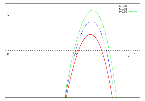
Figure 2: Effective potential for different comoving radii in Case A type configuration. Here $m_{0}=1.25$, $p_{\theta_{2}}=4.5$, $b_{0}=-3.0$ and $m_{2}=0.1.$

Case B

As $m_{0}$ is increased further, we reach a value at which the potential for the central shell just touches the $x$ axis. We call this value as the critical value $m_{0c}$ of the initial parameter $m_{0}$ (for the other two parameters fixed). This is shown in FIG. 3. The outer shells still have positive potential which indicates forbidden region, therefore, all those shells will bounce back. This configuration is the boundary point between the complete dispersal and black hole formation.

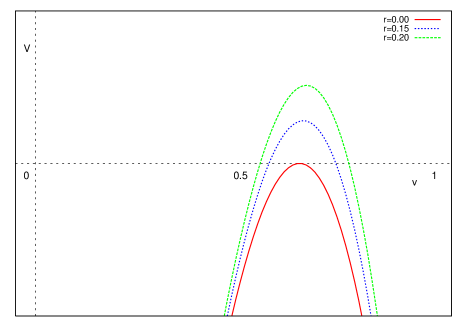
Figure 3: Effective potential for different comoving radii for Case B type configuration. Here $m_{0}=1.3333$, $p_{\theta_{2}}=4.5$, $b_{0}=-3.0$ and $m_{2}=0.1.$

Case C

If we increase $m_{0}$ even further, the potential for the central shell (FIG. 4) is negative for the whole range of $v$ which will allow the central shell to reach the singularity at $v=0$. If we increase $r$, the potential minima goes up, and there is a value of $r$ at which the effective potential just touches the $x$ axis. We call this radius the critical radius $r_{c}$ of the collapsing cloud for the chosen set of initial numbers. Now all the shells from $r=0$ to $r=r_{c}$ will reach the singularity and will contribute to the mass of the black hole formed, but the shells with comoving coordinate more than $r_{c}$ bounce off. We numerically confirm this by integrating equation (15). Physical radius for various shells is plotted in FIG. 5.

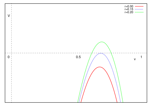
Figure 4: Effective potential for different comoving radii in Case C type configuration. Here $m_{0}=1.40$, $p_{\theta_{2}}=4.5$, $b_{0}=-3.0$ and $m_{2}=0.1.$

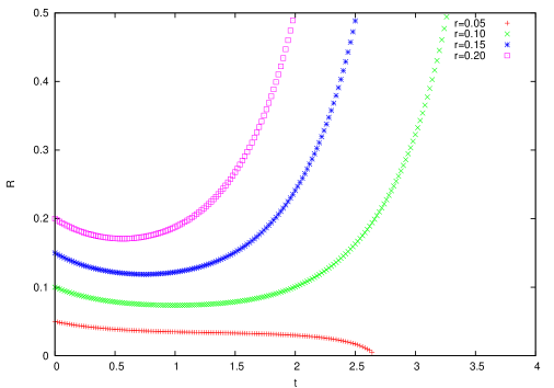
Figure 5: Physical radius of different shells in Case C type evolution, where $m_{0}=1.35,|b_{0}|=3.0$, $m_{2}=0.1$ and $p_{\theta_{2}}=4.5$. Shells with comoving radius less than the critical radius reach singularity, while those with larger than critical value escape to infinity.

We can understand qualitatively why the solution for Case B is a massless naked singularity. Suppose we are in initial data parameter range of Case C regime and we decrease the value of $m_{0}$. As $m_{0}$ approaches $m_{0c}$ fewer and fewer shells reach singularity. Thus if we approach the threshold of black hole formation from the initial data of Case C region, we can see that when $m_{0}$ is very very close to $m_{0c}$, almost only the central shell reaches singularity and other shells are stopped from collapsing and bounce back at the value of $v$ which is the root of the potential for those shells. Apparent horizon is given by equation $F=R$, which implies $v_{ah}\approx r^{2}\,m_{0}$ for the shells near the center. A shell is trapped if it reaches value of $v$ smaller than $v_{ah}$. Now, as all outer shells reach a minimum value $v_{0}(r)>>v_{ah}$, those are not trapped. Only the central shell is singular when $m_{0}$ is nearly equal to $m_{0c}$ and trapped surfaces are not formed. As $F=r^{3}{\cal M}(r)$, the mass which contributes towards singularity formation is zero which means the singularity is massless and also as the trapped surfaces are not formed, the central singularity is visible.

We note that in the collapsing cloud if a shell bounces then all the shells with larger value of comoving radius will also bounce, i.e. there is no shell-crossing. To see this, we can integrate near the center numerically to obtain $R^{\prime}$ as well as all the metric functions. We see that $R^{\prime}$ remains positive during the collapse evolution which is plotted for one particular initial data set in FIG. 6. We find all solutions for various values of initial data and it was seen that for the critical solution as well as for solutions near the critical point shell cross does not occur.

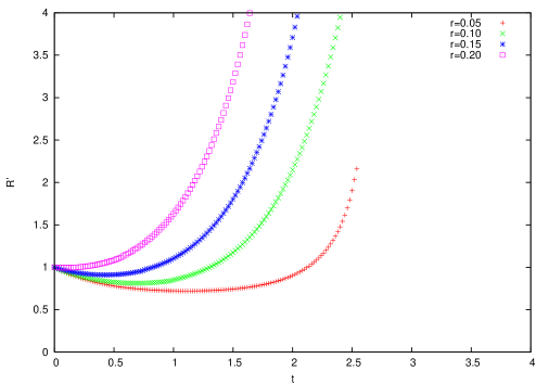
Figure 6: $R^{\prime}$ for different shells in Case C type evolution, where $m_{0}=1.35,|b_{0}|=3.0$, $m_{2}=0.1$ and $p_{\theta_{2}}=4.5$.

The expression for critical radius in terms of the initial parameters can be obtained from the condition that at critical radius, effective potential just touches the $x$ axis, i.e. the quintic polynomial has double roots. For a quintic polynomial $a_{5}x^{5}+a_{3}x^{3}+a_{1}x+a_{0}=0$ , the discriminant is given as follows pari ,

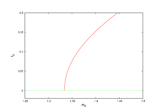
Figure 7: Figure represents behavior of critical radius with the density parameter, keeping other parameters values unchanged.

$$\Delta=a_{5}\left[a_{0}^{2}(108a_{3}^{5}-900a_{1}a_{3}^{3}a_{5}+2000a_{1}^{2}a_{3}a_{5}^{2}+3125a_{0}^{2}a_{5}^{3})+16a_{1}^{3}a_{3}^{4}-128a_{1}^{4}a_{3}^{2}a_{5}+256a_{1}^{5}a_{5}^{2}\right].$$ (17)

The condition that $\Delta$ vanishes at the double root gives, from equation (16), the expression for critical radius as,

$$r_{c}^{2}=\frac{m_{0}-m_{0c}}{m_{0}(0.833b_{0}+2m_{2})+c_{1}(0.22b_{0}^{3}-1.04m_{0}p_{\theta_{2}})},$$ (18)

where $c_{1}=\frac{b_{0}m_{0}}{p_{\theta_{2}}^{2}}(3p_{\theta_{2}}+10m_{2})$ and $m_{0c}=\frac{2b_{0}^{3}}{9p_{\theta_{2}}}$. Behavior of the critical radius with the parameter $m_{0}$ can be seen in FIG.7. In the model considered here, the mass function, which is twice the Misner-Sharp mass, depends only on $r$. The total mass which collapsed to form singularity from the regular initial profile is $\frac{1}{2}r_{c}^{3}m_{0}e^{-m_{1}r_{c}^{2}}$. The mass of black hole would then be

$$M_{BH}=c_{m}(m_{0}-m_{0c})^{\frac{3}{2}},$$ (19)

where $c_{m}$ is a constant near the threshold. We can fix any of the two parameters $m_{0}$, $b_{0}$, and $p_{\theta_{2}}$ and vary the third one to obtain the expression for critical radius. Following the same procedure as earlier, it is easily seen that for $b_{0}$ and $p_{\theta_{2}}$ the same scaling relation and exponent exists near the threshold of the black hole formation. Therefore, in general, for a parameter $\xi$, we can write $M_{BH}=c_{\xi}|\xi-\xi_{c}|^{\frac{3}{2}}$.

V Discussion and Conclusions

We like to point out the similarities in the behaviour of this model with the critical behavior in scalar field gravitational collapse choptuik , and other matter models radiation :

i) The three types of evolutions discussed in Case A-C are very much analogous to the subcritical, Critical and super-critical evolutions studied in the above models. In case A the whole cloud disperse off and in Case C black hole forms whose mass can be controlled by an initial parameter. Case B is the boundary between the case A and Case C configuration which is like the critical solution in the above cases.

ii) A power law behaviour is seen for the mass of the black hole near the threshold of its formation. Infinitesimal mass black holes can be formed in this model if the initial parameters are finely tuned.

iii) The same value of exponent is observed for different initial parameters which is like universality of the critical solution.

Our purpose here is to investigate how the initial parameters determine the evolution and the end state of collapse. The metric function $\nu$, in spite being a restrictive choice, makes the model tractable. The other class of tangential pressure models, i.e non-static Einstein cluster has a different form of the function $\nu$ in comoving coordinates and it can not be written as function of $R$ only. We have observed similar behavior at threshold of black hole formation in Einstein cluster as well and the same value of the exponent was seen mahajan . The effective potential method for calculating the critical exponent applies to this case as well as to non-static Einstein cluster mahajan . This suggests that the method applies at least for all mass-conserving systems. However, the system considered here has a limitation, and is different from the models considered so far for critical behaviour in one respect that it has no radial stress which enables shells to interact directly with each other. It will be interesting to explore whether the method we used here could be applied for studying such behaviour in the models with a non-vanishing radial pressure as well.

Acknowledgments

S. Gutti, R. Goswami and A. Madhav are thanked for useful discussions.

APPENDIX A : BLACK HOLE FORMATION FOR COLLAPSE IN CASE C CONFIGURATION

We can rewrite equation (12) as

$$\sqrt{v}\dot{v}=-\sqrt{e^{4\nu_{0}}vb_{0}+e^{2\nu_{0}}\left(v^{3}h(rv)+{\cal M}\right)},$$ (20)

where

$$h(R)=\frac{e^{2\nu_{0}(R)}-1}{R^{2}}.$$ (21)

Integrating the above equation, we get

$$t(v,r)=\int_{v}^{1}\frac{\sqrt{v}dv}{\sqrt{e^{4\nu_{0}}vb_{0}+e^{2\nu_{0}}\left(v^{3}h(rv)+{\cal M}\right)}}$$ (22)

The time of singularity for a shell at a comoving coordinate radius $r$ is the time when the physical radius $R(r,t)$ becomes zero. The shells collapse consecutively, that is one after the other to the center as there are no shell-crossings. Taylor expanding the above function around $r=0$, we get

$$t(v,r)=t(v,0)\;+\left.r\;\frac{dt(v,r)}{dr}\right|_{r=0}+\left.\frac{r^{2}}{2!}\;\frac{d^{2}t(v,r)}{d^{2}{r}^{2}}\right|_{r=0}$$ (23)

Let us denote

$${\cal X}_{n}(v)=\left.\frac{{d}^{n}t(v,r)}{{d}r^{n}}\right|_{r=0}$$ (24)

As we have taken the initial data with only even powers of $r$, the first derivatives of the functions appearing in above equations vanish at $r=0$, hence we have

$${\cal X}_{1}(v)=0$$ (25)

Now we can express the next coefficient ${\cal X}_{2}$ as

$${\cal X}_{2}(v)=-\int_{v}^{1}\frac{\sqrt{v}dv[\beta v^{5}+2m_{0}p_{\theta_{2}}v^{2}+9m_{0}^{2}(b_{02}v+m_{2})]}{9m_{0}^{2}\,(hv^{3}+b_{00}v+M)^{\frac{3}{2}}}$$ (26)

where

$$\beta=6p_{\theta_{2}}^{2}+24m_{0}b_{02}p_{\theta_{2}}-3m_{0}\rho_{2}p_{\theta_{2}}$$ (27)

We need to determine now whether it is possible to have families of future directed outgoing null geodesics coming out of the singularity. In the case when such families do exist which terminate in the past at the singularity, and which could reach outside observers, then the singularity will be visible. In the case otherwise it is hidden within the black hole. Another way to look at this is through the apparent horizon and formation of trapped surfaces in the spacetime. As the collapse evolves, if the trapped surfaces form well in advance to the formation of the singularity, then the same will be covered. On the other hand, if the trapped surface formation is sufficiently delayed during the collapse then the singularity may be naked. The apparent horizon within the collapsing cloud is given by the equation , $R/F=1$, which gives the boundary of the trapped surface region of the space-time. If the neighborhood of the center gets trapped earlier than the singularity, then it is covered, otherwise it is naked with non-spacelike future directed trajectories escaping from it.

In order to consider the possibility of existence of such families, and to examine the nature of the singularity occurring at $R=0,r=0$ in this model, let us consider the outgoing null geodesic equation which is given by

$$\frac{dt}{dr}=e^{\psi-\nu}$$ (28)

We now use here a method which is similar to that given in dim . The singularity curve is given by $v(t_{s}(r),r)=0$, which corresponds to $R(t_{s}(r),r)=0$. Therefore, if we have any future directed outgoing null geodesics terminating in the past at the singularity, we must have $R\rightarrow 0$ as $t\rightarrow t_{s}$ along the same. Now writing equation (28) in terms of variables $(u=r^{\alpha},R)$, we have

$$\frac{dR}{du}=\frac{1}{\alpha}r^{-(\alpha-1)}R^{\prime}\left[1+\frac{\dot{R}}{R^{\prime}}e^{\psi-\nu}\right]$$ (29)

Now in order to get tangent to the null geodesic in the $(R,u)$ plane, we choose a particular value of $\alpha$ such that the geodesic equation is expressed only in terms of $\left(\frac{R}{u}\right)$. A specific value of alpha is to be chosen which enables us to calculate the proper limits at the central singularity. For example, for ${\cal X}_{1}(0)\neq 0$ case, we can choose $\alpha=\frac{5}{3}$ and using equation (5), (and considering that $\dot{R}<0$), we get

$$\frac{dR}{du}=\frac{3}{5}\left(\frac{R}{u}+\frac{\sqrt{{\cal M}_{0}}{\cal X}_{1}(0)}{\sqrt{\frac{R}{u}}}\right)\left(\frac{1-\frac{F}{R}}{\sqrt{G}[\sqrt{G}+\sqrt{H}]}\right)$$ (30)

In the tangential pressure collapse model discussed in the previous section we have ${\cal X}_{1}(0)=0$, and hence we choose $\alpha=\frac{7}{3}$ so that when in limit $r\rightarrow 0,t\rightarrow t_{s}$ we get the value of tangent to null geodesic in the $(R,u)$ plane

$$\frac{dR}{du}=\frac{3}{7}\left(\frac{R}{u}+\frac{\sqrt{M_{0}}{\cal X}_{2}(0)}{\sqrt{\frac{R}{u}}}\right)\frac{(1-\frac{F}{R})}{\sqrt{G}(\sqrt{G}+\sqrt{H})}$$ (31)

Now note that for any point with $r>0$ on the singularity curve $t_{s}(r)$, we have $R\to 0$ whereas $F$ (interpreted as mass of the object within the comoving radius $r$) tends to a finite positive value once the energy conditions are satisfied. Under the situation, the term $F/R$ diverges in the above equation, and all such points on the singularity curve will be covered as there will be no outgoing null geodesics from such points.

Hence we need to examine the central singularity at $r=0,R=0$ to determine if it is visible or not. That is, we need to determine if there are any solutions existing to the outgoing null geodesics equation, which terminate in the past at the singularity and in future go to a faraway observer, and if so under what conditions these exist. Note that if any outgoing null geodesics terminate at the singularity in the past then along the same, in the limit as $r\rightarrow 0,t\rightarrow t_{s}$ we then have from equation (26) $\dot{R}=0$, therefore $H=0$ and $G=1$ in this limit as $F/R$ vanishes. Let now $x_{0}$ be the tangent to the null geodesics in $(R,u)$ plane, at the central singularity, then it is given by,

$$x_{0}=\lim_{t\rightarrow t_{s}}\lim_{r\rightarrow 0}\frac{R}{u}=\left.\frac{dR}{du}\right|_{t\rightarrow t_{s};r\rightarrow 0}$$ (32)

Using equation (31), we get,

$$x_{0}^{\frac{3}{2}}=\frac{7}{4}\sqrt{{\cal M}_{0}}{\cal X}_{2}(0)$$ (33)

In the $(R,u)$ plane, the null geodesic equation will be,

$$R=x_{0}u$$ (34)

It follows that if ${\cal X}_{2}(0)>0$, then that implies that $x_{0}>0$, and we then have radially outgoing null geodesics coming out from the singularity, making the central singularity to be a visible one. On the other hand, if ${\cal X}_{2}(0)\leq 0$, we will have a black hole solution. Now for the initial data in the range of Case C, we calculate ${\cal X}_{2}(0)$ and find that it remains negative which implies that a black hole is necessarily formed.

References

- (1) Einstein A., Ann. Math. 40, 4 922 (1939)
- (2) Datta B. K., Gen. Relat. Grav. 1, 19 (1970); Bondi H., Gen. Relat. Grav. 2, 321 (1971).
- (3) G. Magli, Class. Quant. Grav. 14 (1997) 1937; Class. Quant. Grav. 15 (1998) 3215;
- (4) S. M. C. V. Goncalves, S. Jhingan, G. Magli, Phys.Rev. D65 (2002) 064011; T.Harada, K.Nakao and H.Eguchi, Class.Quantum Grav. 16(1999) 2785-2796; A.Mahajan, R.Goswami and P.S. Joshi, Class.Quantum Grav. 22(2005) 271-282.
- (5) C.R.Evans and J.S.Colman, Phys.Rev.Lett. 72 (1994) 1782; D.W.Neilsen and M.W.Choptuik, Class.Quant.Grav. 17,(2000) 761; C.Gundlach, Phys.Rev. D55 (1997) 6002; D.Eardly,E.Hirschmann and J.Horne, Phys.Rev. D52 (1995) 5397.
- (6) S. W. Hawking and G. F. R. Ellis, The large scale structure of spacetime, Cambridge Univ. Press, Cambridge (1973).
- (7) C.W.Misner and D.H.Sharp, Phys.Rev 136 B571 (1964).
- (8) A. Frolov, Class. Quant. Grav. 16 (1999) 407
- (9) Dickson L. E., New First Course in the Theory of Equations, John Wiley & sons, New York.
- (10) C.Batut, D.Bernardi, H.Cohen, M.Olivier PARI-GP, Version 2.2.12.
- (11) M.W.Choptuik, Phys.Rev.Lett.70, 9 (1993).
- (12) A.Mahajan, T.Harada, P.S.Joshi and K.Nakao, submitted for publication.
- (13) R. Goswami and P. S. Joshi, Phys. Rev. D69 (2004) 044002; R. Goswami and P. S. Joshi, Phys. Rev. D69 (2004) 104002.