Cauchy–perturbative matching revisited: tests in spherical symmetry

Abstract

During the last few years progress has been made on several fronts making it possible to revisit Cauchy–perturbative matching (CPM) in numerical relativity in a more robust and accurate way. This paper is the first in a series where we plan to analyze CPM in the light of these new results.

One of the new developments is an understanding of how to impose constraint-preserving boundary conditions (CPBC); though most of the related research has been driven by outer boundaries, one can use them for matching interface boundaries as well. Another front is related to numerically stable evolutions using multiple patches, which in the context of CPM allows the matching to be performed on a spherical surface, thus avoiding interpolations between Cartesian and spherical grids. One way of achieving stability for such schemes of arbitrary high order is through the use of penalty techniques and discrete derivatives satisfying summation by parts (SBP). Recently, new, very efficient and high order accurate derivatives satisfying SBP and associated dissipation operators have been constructed.

Here we start by testing all these techniques applied to CPM in a setting that is simple enough to study all the ingredients in great detail: Einstein’s equations in spherical symmetry, describing a black hole coupled to a massless scalar field. We show that with the techniques described above, the errors introduced by Cauchy–perturbative matching are very small, and that very long term and accurate CPM evolutions can be achieved. Our tests include the accretion and ring-down phase of a Schwarzschild black hole with CPM, where we find that the discrete evolution introduces, with a low spatial resolution of $\Delta r=M/10$, an error of $0.3\%$ after an evolution time of $1,000,000\,M$. For a black hole of solar mass, this corresponds to approximately $5\,s$, and is therefore at the lower end of timescales discussed e.g. in the collapsar model of gamma-ray burst engines.

I Introduction

It is generally expected that the geometry of compact sources should resemble flat spacetime at large enough distances. This is true not only qualitatively, but through very precise falloff conditions that are built into the formal definition of asymptotic flatness. Within this definition, the deviations from flat spacetime are well described (in the sense of the leading order behaviour of an expansion in powers of “$1/r$”) by perturbations of the Schwarzschild spacetime Misner et al. (1973).

Such perturbations can in turn be studied through the gauge invariant Regge-Wheeler and Zerilli (RWZ) formalisms Regge and Wheeler (1957); Zerilli (1970). These allow one to derive, after a spherical harmonic decomposition (that is, for each “$(\ell,m)$”), two master evolution equations for the truly gauge invariant, linearized physical degrees of freedom. Due to the multipole decomposition, these equations involve only one spatial coordinate (the radial one). The fact that they are one-dimensional implies that these master equations can be solved for very large computational domains with very modest computational resources. On the other hand, three-dimensional Cauchy codes are very demanding on their resource requirements. Even though mesh refinement can help in this respect, there is a limit to how much one can coarsen the grid in the asymptotic region; this limit is set by the resolution required to reasonably represent wave propagation in the radiative zone. The use of a grid structure adapted to the physical geometry (possibly through multiple patches) can also help Lehner et al. (2005a); Thornburg (2004); Kidder et al. (2001), but one still ends up imposing artificial (even if constraint-preserving) boundary conditions at the outer boundary. For example, one in general misses information about the geometry outside the domain Lau (2005).

Two approaches that at the same time provide wave extraction, physically motivated boundary conditions, and extend the computational domain to the radiative regime are Cauchy–characteristic Winicour (2005); Bishop et al. (1996) and Cauchy–perturbative matching (CPM) Rezzolla et al. (1999); Rupright et al. (1998); Gómez et al. (1998); this paper is concerned with the latter. The idea is to match at each timestep a fully non-linear Cauchy code to an outer one solving, say, the RWZ equations.

This paper is the first one in a series where we plan to revisit CPM in the light of some recent technical developments —which we describe below— that should help in its implementation. Before discussing these developments, we point out and summarize some features present in the original implementation of CPM which we hope to improve on:

1. The non-linear Cauchy equations were solved on a Cartesian, cubic grid. On the other hand, the RWZ equations use a radial coordinate for the spatial dimension. Mixing Cartesian coordinates with spherical ones leads to the need for interpolation back and forth between both grids. Especially when using high order methods, this type of interpolation might not only be complicated but also subtle: depending on how it is done it might introduce noise and sometimes it might even be a source of numerical instabilities.

2. When injecting data from the perturbative module to the Cauchy code and vice versa boundary conditions were given to all modes, irrespectively of their propagation speed and without taking into account the existence of constraint violating boundary modes. One would intuitively expect a cleaner matching if boundary conditions are given according to the characteristic (propagation) speeds of the different modes, and even cleaner if constraint-preservation is automatically built in during the matching.

3. Low order numerical schemes, which result in slow convergence, were used.

In recent years there has been progress on several related fronts that should in principle help in the implementation of CPM. We describe these new results next:

1. The first improvement is the ability to implement smooth (in particular, spherical) boundaries in 3D Cauchy evolutions Lehner et al. (2005a); Thornburg (2004); Kidder et al. (2001). One important advantage of this is the fact that the matching can be performed —to either a perturbative or a characteristic outer module— without the need for interpolation between spherical and Cartesian grids. In that way a possible source of noise can be eliminated. It is now understood how to match different domains using schemes of arbitrary high order while at the same time ensuring numerical stability. One way of doing so is through the use of multiple patches (much in the same way multiple charts are used in differential geometry), penalty terms and difference operators satisfying summation by parts Lehner et al. (2005a) (more about this below). This is the approach we shall explore here in the context of CPM.

2. The second improvement is the construction of constraint-preserving boundary conditions (CPBC). Several efforts have by now reported numerically stable (in the sense of convergent) implementations of such boundary conditions for the fully three-dimensional non-linear Einstein’s equations Sarbach and Tiglio (2004); Kidder et al. (2005); Szilagyi and Winicour (2003). Furthermore, there have been reports in the context of Cauchy–characteristic matching that significant improvements are obtained when this type of boundary conditions are used in the matching Szilagyi and Winicour (2003). With this in mind, we will test their use in CPM.

3. Lastly, new, accurate and efficient high order difference operators satisfying SBP and associated dissipative operators have been constructed recently Strand (1994, 1996); Mattsson et al. (2004); Diener et al. (2005). As mentioned above, in conjunction with certain penalty interface treatment such operators guarantee numerical stability when “glueing” together different computational grids. We will test these operators in the context of CPM.

We have incorporated these techniques, i.e., high-order summation-by-parts finite differencing and dissipation operators, multiple coordinate patches with penalty inter-patch constraint-preserving boundary conditions and Cauchy–perturbative matching, into a spherically symmetric numerical code evolving the Einstein–Christoffel form of the field equations Anderson and York (1999), minimally coupled to a Klein-Gordon field. Using this tool, we can test the performance of the numerical methods in a non-trivial, but easily reproducible and computationally inexpensive setting, and gain experience for three-dimensional applications. The evolutions presented here model black holes with excision in isolation, under dynamical slicings, and black holes accreting scalar field pulses, which are used as a scalar analogue of gravitational radiation.

The plan of this paper is as follows. In section II we introduce the continuum system and the numerical techniques we have used. Results are presented in section III, where a black hole is evolved successively from simple settings, i.e., single-patch, isolated, Killing-field adapted gauges, to more involved ones including Cauchy–perturbative matching and scalar pulse accretion. Finally, in section IV, we draw conclusions and give an outlook to future work.

II Equations and Methods

II.1 Evolution equations and constraint-preserving boundary conditions

In this paper we use the Einstein–Christoffel (EC) system Anderson and York (1999) in spherical symmetry. We follow the notation of Ref. Kidder et al. (2000); in particular, the densitized lapse is denoted by $\alpha=Ng^{-1/2}$, and $\tilde{\alpha}=\alpha r^{2}\sin(\theta)$ is introduced for convenience. Here, $g$ is the determinant of the 3-metric and $N$ the lapse function, while the 4-metric is written as

$$ds^{2}=-N^{2}dt^{2}+g_{rr}(dr+\beta dt)^{2}+r^{2}g_{T}(d\theta^{2}+\sin^{2}\theta d\phi^{2})$$

The vacuum part of the evolution equations in spherical symmetry for this formulation constitute a symmetric hyperbolic system of six first order differential equations. The vacuum variables are the two metric and extrinsic curvature components

$$g_{rr},\ g_{T},\ K_{rr},\ K_{T},$$

where the extrinsic curvature is written as

$$K_{ij}=K_{rr}dr^{2}+r^{2}K_{T}(d\theta^{2}+\sin^{2}\theta d\phi^{2}),$$

plus two auxiliary variables needed to make Einstein’s equations a first order system. These extra variables are defined as

$$f_{rrr} = \frac{g^{\prime}_{rr}}{2}+4\frac{g_{rr}f_{rT}}{g_{T}},$$

$$f_{rT} = \frac{g^{\prime}_{T}}{2}+\frac{g_{T}}{r}.$$

In addition, a massless Klein-Gordon field is minimally coupled to the geometry Kidder et al. (2001); Calabrese et al. (2002). The scalar field equation

$$g^{ab}\nabla_{a}\nabla_{b}\Psi=0$$

is converted into a first order system by introduction of the variables

$$\Pi = \frac{1}{N}(\beta\Psi^{\prime}-\dot{\Psi}),$$

$$\Phi = \Psi^{\prime}.$$

Throughout this paper the ’prime’ and ’dot’ represent partial derivatives with respect to $r$ and $t$, respectively.

Constraint preserving boundary conditions are imposed by analyzing the characteristic modes of the main and constraint evolution systems, as discussed in Calabrese et al. (2002). These modes and their associated characteristic speeds are summarized in Table 1. For illustration purposes, we also show the direction of propagation of each mode in the Schwarzschild spacetime in Painlevé-Gullstrand coordinates Painleve (1921); Gullstrand (1922); Martel and Poisson (2001).

Mode	Speed	r<2M	r>2M
$u_{1}=g_{rr}$	$\beta$	left	left
$u_{2}=g_{T}$	$\beta$	left	left
$u_{3}=K_{rr}-f_{rrr}\,g_{rr}^{-1/2}$	$\beta+\tilde{\alpha}\,g_{T}$	left	left
$u_{4}=K_{T}-f_{rT}\,g_{rr}^{-1/2}$	$\beta+\tilde{\alpha}g_{T}$	left	left
$u_{5}=K_{rr}+f_{rrr}\,g_{rr}^{-1/2}$	$\beta-\tilde{\alpha}g_{T}$	left	right
$u_{6}=K_{T}+f_{rT}\,g_{rr}^{-1/2}$	$\beta-\tilde{\alpha}g_{T}$	left	right
$u_{7}=\Pi+\Phi\,g_{rr}^{-1/2}$	$\beta-\tilde{\alpha}g_{T}$	left	right
$u_{8}=\Pi-\Phi\,g_{rr}^{-1/2}$	$\beta+\tilde{\alpha}g_{T}$	left	left

Table 1: Characteristic modes for Einstein-Christoffel system in spherical symmetry, and their direction of propagation for a Schwarzschild spacetime in Painlevé-Gullstrand coordinates with respect to the vector field $\partial_{r}$. In this gauge, all modes are outflow at the inner boundary, if it is located at $r<2M$, while boundary conditions have to be applied to the incoming modes $u_{1},u_{2},u_{3},u_{4}$ and $u_{8}$ at the outer boundary, assuming is is located at $r>2M$.

From Table 1 we notice that for the Schwarzschild spacetime there are four ingoing and two outgoing gravitational modes at the outer boundary, and therefore expect the same count to hold for perturbations thereof. Boundary conditions for the incoming modes $u_{1},u_{2}$ and $u_{4}$ are fixed by the CPBC procedure. Thus, the only free incoming modes are $u_{3}$, which represents a gauge mode and $u_{8}$, which represents a physical one (see Calabrese et al. (2002) for more details). Boundary conditions do not need to be specified at the inner boundary if it is located inside the event horizon, because all modes are outflow then.

II.2 Cauchy–perturbative matching

Since there is no radiative degree of freedom in spherically symmetric spacetimes, we use the massless Klein-Gordon field as a scalar analogue of gravitational waves. To emulate the setup of three-dimensional Cauchy–perturbative matching as closely as possible, the scalar wave is evolved on a fixed Schwarzschild background in a “perturbative” patch defined for $r\geq{r_{m}}$, while the fully non-linear Einstein’s equations are evolved in the “Cauchy” patch, defined for $r\in[r_{e},r_{m}]$, where $r_{e}$ and $r_{m}$ denotes the excision radius and the matching radius, respectively.

The fact that we are using CPBC allows us to perform a clean matching. From the analytical point of view our matching works in the following way: As mentioned above, after the CPBC procedure, only two free characteristic modes are entering the Cauchy computational domain (at $r=r_{m}$), denoted by $u_{3}$ and $u_{8}$. Since in a very precise sense $u_{3}$ is a gauge mode, we are free to give boundary conditions to it in a very simple way: we just set it to its initial value. Regarding $u_{8}$, we use the "perturbative” value of the same quantity coming from the perturtative domain as counterpart, and communicate these two modes (how this is done at the numerical level is explained below). Similarly, there is only one characteristic mode entering the perturbative domain, which is the linearized version of $u_{7}$. We therefore communicate the non-linear and linear versions of that mode as well.

II.3 Discrete techniques

Given a well-posed initial-boundary value problem for Einstein’s field equations, we construct a stable and accurate discrete system by using operators satisfying the SBP property. In short, a finite difference operator, $D$, satisfies SBP on a computational domain $[a,b]$ discretized using grid points $i=1,\ldots,n$ and a grid spacing $h$ if

$$\langle u,Dv\rangle+\langle v,Du\rangle=\left(uv\right)|_{a}^{b}$$ (1)

holds for all grid functions $u,v$. Here the scalar product, $\Sigma$ is defined in terms of its coefficients $\sigma_{ij}$ by

$$\langle u,v\rangle=h\sum_{i,j=1}^{n}u_{i}v_{j}\sigma_{ij}.$$ (2)

In this paper we use the new, efficient, and accurate high order SBP difference operators and associated dissipation operators constructed in Ref. Diener et al. (2005). Thus, as mentioned, this paper also serves as an extra test of those new operators.

SBP operators are standard centered finite difference operators in the interior of the domain, but the stencils are modified to yield lower order operators in a region close to the boundaries (at the boundary itself the stencil is completely one sided). There are several types of SBP operators depending on the properties of the norm. The simplest are the diagonal norm operators. They have the advantage that SBP is guaranteed to hold in several dimensions by simply applying the 1D operator along each direction and that numerical stability can be guaranteed by discrete energy estimates in a wide range of cases. The main disadvantage is that the order of the operator at and close to the boundary is only half the interior order. We denote the SBP operators by the interior and boundary order and consider here the diagonal operators $D_{2-1}$, $D_{4-2}$, $D_{6-3}$ and $D_{8-4}$. The second type is the restricted full norm operators, where the norm is diagonal at the boundary but has a non-diagonal block in the interior. The advantage of these operators is that the order at and close to the boundary is only one order lower than in the interior, while the disadvantage is that schemes based on these operators may be unstable without the use of dissipation. The restricted full operators we use here are $D_{4-3}$ and $D_{6-5}$.

If the computational domain is split into several sub-domains (“patches”), the discrete representation requires a stable technique to communicate the solution at inter-patch boundaries. We make use of a penalty method Lehner et al. (2005b), which adds a damping term to the right hand side of the evolution equation at the boundary point in a way which retains linear stability. The method has a free parameter, called $\delta$ in Ref. Lehner et al. (2005b), which determines how much the difference between characteristic fields on either side of the inter-patch boundary is penalized. Different values of $\delta$ result in different amount of energy dissipation at the inter-patch boundary and can in principle be chosen so that no energy is dissipated (this is marginally stable). Usually the value of $\delta$ is chosen such that some dissipation of energy occurs. With constant values of $\delta$ the amount of dissipation decreases with resolution.

II.4 Numerical code

For the purposes of this paper, a one-dimensional code which supports constraint-preserving boundaries, multiple grid patches, and the use of the aforementioned high order SBP derivative and dissipation operators has been developed. In addition, the code is able to reproduce the (single grid and without CPM matching) second-order methods of Ref. Calabrese et al. (2002) for comparison. We use the methods of lines, and the time integration is performed by a 4th order Runge-Kutta method. The grid patches that we consider here are not intersecting, but touching. This implies, that each grid function is double valued at the patch interface coordinate since the SBP derivative operators are one sided at the boundaries. To ensure consistency without compromising (linear) stability, we make use of a penalty method as described above. Constraint-preserving boundary conditions require the calculation of derivatives of certain grid functions at the outer boundary, which we also obtain by using the SBP derivative operators.

In a black hole setting, the computational domain next to the excision boundary tends to quickly amplify high frequency noise, which can not be represented accurately on the discrete grid. This is especially true for high order accurate derivative operators. Thus, high order simulations of black holes need a certain amount of numerical dissipation to be stable. This dissipation is here provided by the SBP dissipation operators constructed in Ref. Diener et al. (2005). The free parameters of these operators, namely the coefficient of the dissipation and the extent of the transition region (for non-diagonal operators), are found by numerical experiment.

III Results

The numerical experiments presented in this section are set up to systematically test the performance of the new techniques in several situations of increasing difficulty. We start with a series of tests evolving a Schwarzschild black hole in Painlevé-Gullstrand coordinates with either a single patch or two patches matched via the penalty method, and compare the performance of all SBP operators with the second order finite-differencing method presented in Calabrese et al. (2002). Next, to test more dynamical situations, a gauge or scalar field signal is injected in a constraint-preserving manner through the outer boundary and accreted onto the black hole. A robust stability test is then performed with noise on the incoming gauge mode $u_{3}$, and, with Cauchy–perturbative matching, on the scalar field mode $u_{8}$. Finally, a series of high-precision tests involving all techniques are presented, in which a black hole accretes a scalar field injected through the outer boundary of the perturbative patch. These simulations also include a test of the long-term stability and accuracy after accretion and ring-down.

III.1 Schwarzschild black hole in Painlevé-Gullstrand coordinates

In our first series of tests, a Schwarzschild black hole is evolved with high-order accurate SBP operators, constraint-preserving boundary conditions and excision. Cauchy–perturbative matching is not used in these tests. To fix the coordinate system, we make use of the horizon-penetrating Painlevé-Gullstrand coordinates Gullstrand (1922); Martel and Poisson (2001), and we fix the coordinate functions $\tilde{\alpha}$ and $\beta$ of the previous section to their exact values.

For all tests, the inner boundary is located well inside the event horizon (more precisely, it is located at $r_{e}=1M$), which implies that all modes are outflow. Therefore, no boundary conditions may be applied at the excision boundary. The exact boundary location is not crucial as long as it is inside the apparent horizon, but this choice facilitates comparison with Calabrese et al. (2002). Also, in dynamical situations the apparent horizon location may move significantly on the coordinate grid, and to ensure outflow conditions at the inner boundary some penetration into the black hole is of advantage. To match the setup of Calabrese et al. (2002), we set the outer boundary to $r=10M$. To ensure well-posedness of the continuum problem, boundary conditions should be applied to the incoming modes $u_{1}$, $u_{2}$, $u_{3}$, $u_{4}$, and $u_{8}$. However, three of these modes, namely $u_{1}$, $u_{2}$, and $u_{4}$, can be fixed by the use of constraint-preserving boundary conditions, as discussed in Section II, which leaves the freely specifyable gauge mode $u_{3}$ and the scalar field mode $u_{8}$. Since in these initial tests we are only interested in obtaining a stationary black hole solution, the initial scalar field is set to zero, and the (scalar field) characteristic mode $u_{8}$ is penalized to zero as well. The incoming gauge mode $u_{3}$ is penalized to the exact solution.

An error function $\delta M$ can be defined by use of the Misner-Sharp mass function Misner et al. (1973)

$$M(r):=\frac{rg_{T}}{2}\left[1+\frac{r^{2}}{g_{T}}\left(K_{T}^{2}-\frac{f_{rT}^{2}}{g_{rr}}\right)\right],$$ (3)

where then, if the black hole mass is denoted by $M$, $\delta M(r)=(M(r)-M)/M$. Since the same error measure and continuum system is used in Calabrese et al. (2002), we can compare the different discrete approaches directly.

III.1.1 One grid patch

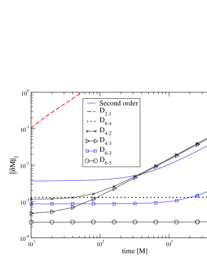
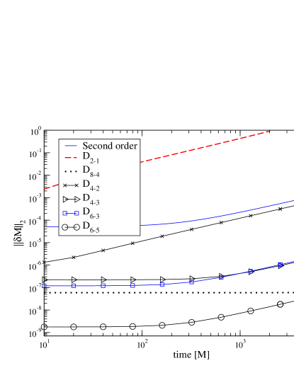
Figure 1: Time evolution of the relative error in the Misner-Sharp mass function when evolving a Schwarzschild black hole in Painlevé-Gullstrand coordinates with one grid patch, for different discrete methods. Two resolutions are displayed, corresponding to $\Delta r=M/8$ (upper panel) and $\Delta r=M/64$ (lower panel). The result from the method presented ref. Calabrese et al. (2002) is denoted by “second order”, while new results are marked by the SBP derivative and dissipation operators used. The high-order operators $D_{6-5}$ and $D_{8-4}$ display superior performance already at the lowest resolution.

The computational domain $r\in[1,10]$ is represented by one coordinate patch, which is exactly the same setup as in ref. Calabrese et al. (2002). In Figure 1 we compare for coarse and high resolutions, $\Delta r=M/8,M/64$, the performance of the methods used in ref. Calabrese et al. (2002), namely second order spatial derivatives with fourth order Kreiss-Oliger dissipation (which is set to zero near the boundaries) and a third order extrapolation at the boundaries, with the SBP derivative and dissipation operators $D_{2-1}$, $D_{4-2}$, $D_{4-3}$, $D_{6-3}$, $D_{6-5}$ and $D_{8-4}$. The figure shows the evolution of the $L_{2}$ norm of the Misner-Sharp mass error over an evolution time of $10,000M$. In all cases displayed there is a linear growth in the error after some time. This is an artefact of the discrete representation of the constraint-preserving boundary conditions. We have also performed tests with maximally dissipative boundary conditions: these yield a discrete equilibrium after some time, and thus allow for evolutions of unlimited time. However, since these boundary conditions are not correct for most systems of practical interest, we only make use of this result to point out the source of the linear growth of errors observed, which converges away with increasing resolution.

As soon as the error gets close to $1$, the code encounters an instability, which, in this case, is associated with a migration of the excision boundary outside of the black hole, and consequently ill-posedness of the continuum problem. While this migration could be theoretically avoided by choosing horizon-fixing dynamical coordinate conditions, a solution with this magnitude of error is, in any case, not of practical use.

In the present numerical code, the SBP operators are also used as one-sided derivatives for determining the constraint-preserving boundary conditions, which suggests that the operator $D_{2-1}$, which is only first order at the boundaries, will yield less accurate outer boundary conditions than the third order method in Calabrese et al. (2002). Figure 1 clearly demonstrates this fact. However, the operators $D_{6-3}$, $D_{6-5}$ and $D_{8-4}$ are significantly more accurate than the results presented in ref. Calabrese et al. (2002), and already so at the coarsest resolution. Furthermore, at $\Delta r=M/64$ the SBP operator $D_{6-5}$ induces a solution error of less than $10^{-7}$ (that is, four orders of magnitude smaller than the corresponding errors when using the second order method of Calabrese et al. (2002) with the same resolution) within $10,000M$, which appears sufficiently accurate for many practical purposes.

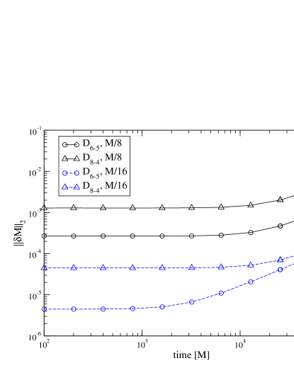
Figure 2: Evolution of a Schwarzschild black hole for $100,000M$. The axes show the quantities described in Figure 1. It is clear that even with low resolutions of $\Delta r=M/8$ and $M/16$, the operators $D_{6-5}$ and $D_{8-4}$ are able to evolve the black hole in a stable manner for a significant time.

The long-term evolution of a Schwarzschild black hole with the operators $D_{6-5}$ and $D_{8-4}$ is displayed in Figure 2. The linear growth of errors dominates the solution at late times, but since this error significantly decreases with resolution, long evolution times can be obtained even for moderate radial grid spacings. This is naturally an interesting feature for simulations with three-dimensional spatial grids, where computational resources are still a viable concern.

III.1.2 Two grid patches

As dicussed in the introduction, the use of multiple coordinate patches has advantages when modelling black holes. To implement a stable interface boundary condition, the penalty method is used to ensure linear stability. Here we first investigate the performance of the SBP operators coupled to an inter-patch penalty boundary method by evolving a black hole spacetime covered by two non-intersecting spherical shells, the first one from $r=1M$ to $r=5.5M$, and the second one from $r=5.5M$ to $r=10M$. In order to provide an intermediate test towards the CPM tests below, we do a non-linear matching, communicating all characteristic modes (that is, without imposing for the moment constraint-preserving boundary conditions at the matching interfaces).

The free parameter of the penalty boundary condition $\delta$ introduced in section II.3 is set to the dissipative value $0$. Only the operators $D_{6-5}$ and $D_{8-4}$ are used for comparison to the results from the previous section.

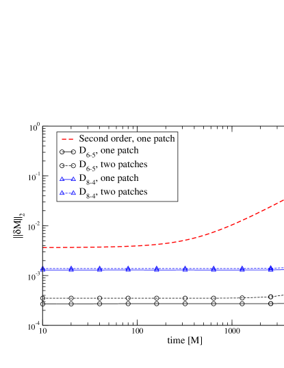
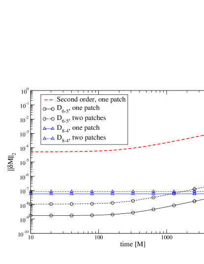
Figure 3: Comparison of uni-patch and multi-patch evolutions of a Schwarzschild black hole in Painlevé-Gullstrand coordinates. The graphs denoted by “one patch” and “second order” are those from Figure 1, while the corresponding graphs for “two patches” cover the computational domain with two non-intersecting spherical shells, the first one from $r=1M$ to $r=5.5M$, and the second one from $r=5.5M$ to $r=10M$. The one-sided derivatives at the interface boundary introduce a very small loss of accuracy. In the upper and lower panels the resolution is $\Delta r=M/8,M/64$, respectively. For the late time behaviour of $D_{6-5}$ and $D_{8-4}$ please also cf. Figure 2.

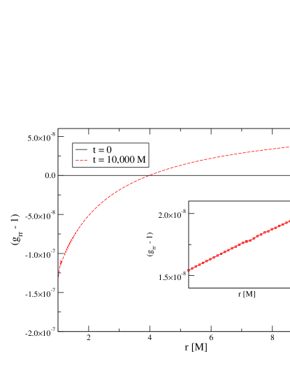
Figure 4: Evolution of metric function $g_{rr}$ for a black hole in Painlevé-Gullstrand coordinates, with a resolution of $\Delta r=M/64$, two grid patches with an interface at $r=5.5M$ and using the SBP operator $D_{6-5}$. The two graphs show the metric function at $t=0$ (where $g_{rr}(r)=1$) and at $t=10,000M$. The inset shows the region around the interface between the grid patches.

In Figure 3 the performance of the multi-patch system is compared to the uni-patch results from the previous section. As expected, the use of one-sided derivatives at the inter-patch boundary reduces the total level of accuracy, but in a very small amount; furthermore, the system is still stable and convergent. The time of the onset of the linear growth observed in all evolutions varies between the grid setups and choices of discrete operator. Figure 4 shows the 3-metric component $g_{rr}(r)$ at the times $t=0$ and $t=10,000M$. The region around the inter-patch interface at $r=5.5M$ is shown in the inset, which demonstrates that the penalty method introduces no strong visible artifacts in this part of the solution. This observation also holds for the other solution functions.

III.2 Gauge wave on a Schwarzschild background

The next series of tests focuses on a dynamical situation, namely the evolution of a Schwarzschild black hole in non-stationary coordinates. For this purpose, the initial data is set to a Schwarzschild black hole in Painlevé-Gullstrand coordinates as in section (III.1), as is the lapse and shift function at all times, but the incoming gauge mode $u_{3}$ at the outer boundary is set to a Gaussian pulse of the form

$$u_{3}(t)=u_{3}^{PG}(1+Ae^{-(t-t_{0})^{2}/\tilde{\sigma}^{2}}).$$ (4)

Here, $u_{3}^{PG}$ is the exact gauge mode from the stationary solution. As in ref. Calabrese et al. (2002), we impose a strong pulse with $A=1$, $t_{0}=5M$ and $\tilde{\sigma}=2M$. Since the solution is now not adapted to the asymptotically timelike Killing field, the SBP operators and multi-patch techniques can be tested on a solution with wave propagation without compromising the use of the error measure $||\delta M||_{2}$. To facilitate comparison with ref. Calabrese et al. (2002), the outer boundary is located at $r=30M$ in these tests.

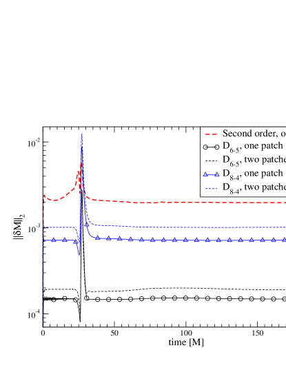
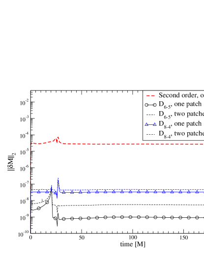
Figure 5: Comparison of uni-patch and multi-patch evolutions of a gauge wave travelling on a Schwarzschild background. The graphs denoted by “second order” are obtained with the methods in ref. Calabrese et al. (2002), while the corresponding graphs for “one patch” and “two patches” cover the computational domain with either one or two non-intersecting spherical shells, the first one from $r=1M$ to $r=15.5M$, and the second one from $r=15.5M$ to $r=30M$. The one-sided derivatives at the interface boundary introduce a small loss of accuracy, but the system is still stable. The upper and lower panels correspond to $\Delta r=M/8,M/64$, respectively.

Figure 5 shows results from the gauge pulse problem on a single grid patch and two grid patches, here with an inter-patch boundary at $r=15.5M$. While in the stationary case the inter-patch boundary method only had to deal with small numerically introduced differences between the values of the geometrical quantities at the interface, the non-stationary case introduces a large pulse travelling over the boundary, and is thus a much more severe test for accuracy and stability of the penalty method. The solution error is dominated by the ability of the discrete method to represent the propagation and accretion of the gauge pulse, and by possible artefacts introduced by the inter-patch boundary.

Judging from Figure 5, the high-order operators are stable and significantly more accurate than a second order method also in a dynamical situation, and even when using multiple matched domains.

III.3 Accretion of a scalar field pulse

Since the outer boundary has two free incoming modes, it is possible to inject a scalar field pulse in a way similar to the gauge pulse of section (III.2). In contrast to the gauge pulse, however, this system will result in an increase of mass of the black hole, which also implies that the Misner-Sharp mass cannot be used as a measure of the errors anymore. A possible choice for a gauge field source with compact support is

$$u_{8}(t)=\left\{\begin{array}[]{ll}0&t<t_{I}\\ \frac{A}{t_{F}^{8}}(t-t_{I})^{4}(t-t_{F})^{4}\sin(\frac{\pi t}{t_{F}})&t\in[t_{I},t_{F}]\\ 0&t>t_{F}\end{array}\right.$$

To facilitate comparisons with ref.  Calabrese et al. (2002) we use an amplitude $A=7.2$, and $t_{I}=0M$, $t_{F}=10M$ and set the computational domain to be $r\in[1,50]M$.

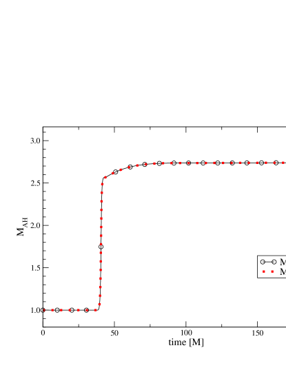
Figure 6: Evolution of the apparent horizon mass for the accretion of a strong scalar pulse to a Schwarzschild black hole. Shown are plots for two resolutions, $\Delta r=M/20$ and $\Delta r=M/40$, using the SBP operator $D_{6-5}$. The large scalar field amplitude leads to a significant increase in the black hole mass.

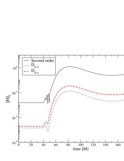
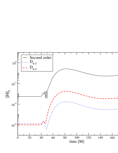
Figure 7: $L_{2}$ norm of the Hamiltonian constraint over time for the accretion of a strong scalar field pulse to a Schwarzschild black hole, with resolutions $\Delta r=M/20,M/40$ (upper and lower panels, respectively). The graph denoted by “second order” is obtained with the method presented in Calabrese et al. (2002), and the $D_{6-5}$ and $D_{8-4}$ are obtained using the corresponding SBP operators.

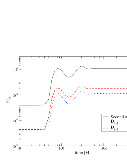
Figure 8: As Figure 7, but evolved for 10,000 M with $\Delta r=M/20$ to demonstrate the long-term behaviour after accretion of the pulse.

For resolutions $\Delta r=M/20$ and $\Delta r=M/40$, the time evolution of the apparent horizon is shown in Figure 6. The scalar pulse leads to a significant increase in the black hole mass by a factor of $\approx 2.7$ after the pulse is inside the black hole. Larger amplitudes are not obtainable with the simple gauge prescription used here, but a horizon-freezing gauge condition could improve on this result. As a replacement for the Misner-Sharp error measure, we plot the $L_{2}$ norm of the Hamiltonian constraint over time in Figure 7. It is apparent that the high-order operators are again stable and more accurate than the second order operator. The graphs indicate a growth of the constraint near $t=200M$, but a long-term evolution with $\Delta r=M/20$ shown in Figure 8 demonstrates that the system settles down to stability after the accretion.

III.4 Robust stability test with gauge noise

The term robust stability test Alcubierre et al. (2004) typically refers to the discrete stability of a numerical system in response to random perturbations. In this case, we will use the same system as in section (III.1.2), but impose random noise on the incoming gauge mode $u_{3}$ with a certain amplitude. To test the discrete stability of the evolution system, we chose a large range of amplitudes from $10^{-4}$ to $0.3$. Random perturbations of the latter amplitude is significant for a non-linear system.

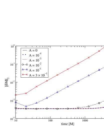
Figure 9: Results of a robust stability test for different random noise amplitudes. The system is a Schwarzschild black hole in Painlevé-Gullstrand coordinates, and the computational domain $r\in[1,10]M$ is covered by two patches with a boundary at $r=5.5M$ and a resolution of $M/8$. Random noise is superimposed on the ingoing gauge mode $u_{3}$, with an amplitude denoted by $A$. The graphs show the mass error with time for different random noise amplitudes, obtained with the SBP operator $D_{6-5}$.

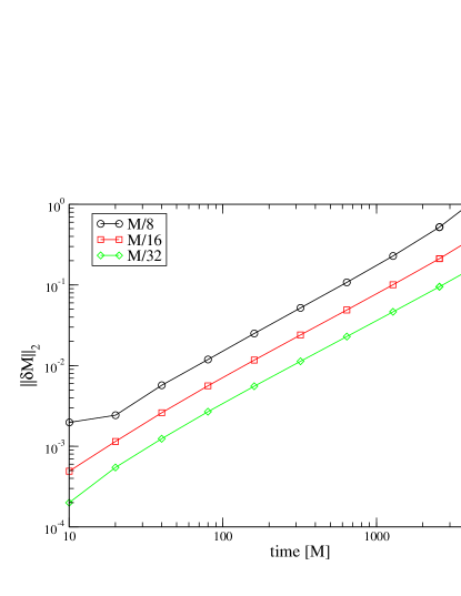
Figure 10: Like Figure 9, but for the highest random noise amplitude $0.3$ and different resolutions.

For this multi-patch test, results in the mass error for a resolution $\Delta r=M/8$ are shown in Figure 9. It is apparent that strong random noise induces a stronger growth in the solution error. However, this growth is still linear. As in all black hole evolutions in section (III.1), the system encounters a numerical instability as the solution error approaches $1$, but this is not a consequence of the random noise, but of the inner boundary becoming partially inflow due to a coordinate motion of the apparent horizon. Also, with increasing resolution, the growth rate of the error does not increase, as shown in Figure 10. We conclude that this high-order evolution system is discretely stable against strong random perturbations.

III.5 Cauchy–perturbative matching: robust stability test with scalar field noise

We now test the stability of the system with Cauchy–perturbative matching against random perturbations in the scalar field. To this end, the computational domain is again subdivided as in section (III.4), but the right patch evolves the scalar field on a fixed Painlevé-Gullstrand background as explained in the introduction. The interpatch boundary is thus matching the Cauchy patch to a perturbative one, and we test the stability of the system against random perturbations by imposing random noise on the incoming scalar field mode on the outer boundary of the perturbative patch.

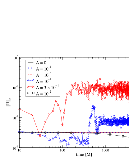
Figure 11: Robust stability test with Cauchy–perturbative matching. The system is a dynamically evolved Schwarzschild black hole in Painlevé-Gullstrand coordinates matched to a perturbative module at $r=5.5M$ as described in the introduction. Random noise is imposed via the incoming scalar field mode at the outer boundary. Plotted is the $L_{2}$ norm of the Hamiltonian constraint over time for different noise amplitudes. All evolutions were done with a resolution of $\Delta r=M/8$ and the SBP operator $D_{6-5}$.

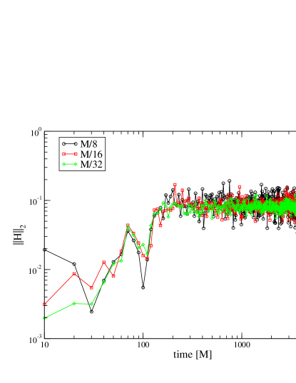
Figure 12: Like Figure 11, but for the highest random noise amplitude and different resolutions.

Since the mass error is not available for a system accreting a scalar field, the $L_{2}$ norm of the Hamiltonian constraint is used again in Figure 11. No exponential growth can be observed in the Hamiltonian constraint violation. The same is true when increasing the resolutions, as in Figure 12, which also deserves some additional comments: The robust stability test does not lead to a converging sequence of solutions if the random noise amplitude is not diminished with resolution. However, the purpose of these tests is to excite any unstable high freqcency modes present in the numerical system. The absence of any mode growing with increasing resolution shows that the system with a Cauchy–perturbative matching interface is stable even against strong random noise injected into the system. This is a promising result for any effort to do three-dimensional matching between Cauchy modules and perturbative ones using multiple patches and high-order summation-by-parts operators.

III.6 Cauchy–perturbative matching: Accretion of a “gravitational wave” and long-term evolution

Finally, using the massless Klein-Gordon field as a scalar analogue of gravitational waves in spherical symmetry, we model the accretion of a gravitational wave packet across a Cauchy–perturbative matching boundary. This test is an extension of the single-patch scalar field accretion of section (III.3), and makes use of all ingredients presented in this paper for a stable and accurate evolution of black holes with Cauchy–perturbative matching.

Figure 13: Accretion of a scalar wave packet across a Cauchy–peturbative matching interface, as a scalar analog for gravitational wave accretion in three-dimensional simulations. The packet consists of 50 waves injected from $t=0$ to $t=100M$, as described in the text. Here, the grid function $\Phi$ is plotted over the radial coordinate at $t=30M,65M,110M$ (from top to bottom), for the resolution $\Delta r=M/20$ and the SBP operator $D_{6-5}$. The inset shows the behaviour of the grid function around the matching interface, which is at $r=25.5M$. Note that even though the grid function is in principle two-valued on the interface, the penalties in conjunction with high order operators only lead to a very small mismatch.

Figure 14: Accretion of a scalar wave packet across a Cauchy–peturbative matching interface. This plot shows the apparent horizon mass over time for evolutions with different resolutions and the SBP operator $D_{6-5}$.

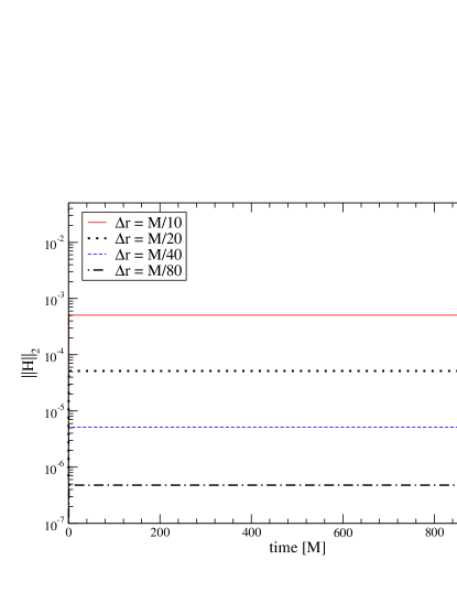
Figure 15: Accretion of a scalar wave packet across a Cauchy–peturbative matching interface. This plot shows the $L_{2}$ norm of the Hamiltonian constraint for different resolutions, using the SBP operator $D_{6-5}$. The non-linear constraint violations introduced at the continuum by the matching are small enough that they cannot be detected in these very accurate simulations. Please note, for comparison with Figure 8, that the amplitude of the Klein-Gordon signal is smaller compared to section (III.3).

Since Cauchy–perturbative matching assumes the gravitational wave to be a small perturbation of a fixed background in the wave zone, the amplitude of the wave packet that we inject through the outermost boundary is chosen to be $A=0.01$. Similarly to section III.3, we describe the packet by the function

$$u_{8}(t)=\left\{\begin{array}[]{ll}0&t<t_{I}\\ \frac{A}{t_{F}^{8}}(t-t_{I})^{4}(t-t_{F})^{4}\sin(\frac{\pi t}{nt_{F}})&t\in[t_{I},t_{F}]\\ 0&t>t_{F}\end{array}\right.$$

where for the number of half waves in the pulse we set $n=100$. We inject the packet from $t_{I}=0$ to $t_{F}=100M$. The plots in Figure 13 display the the evolution of the grid function $\Phi$, and specifically the behaviour of the function around the Cauchy–perturbative matching interface, which is at $r=25.5M$. The corresponding increase in apparent horizon mass is shown in Figure 14. The evolution of the Hamiltonian constraint violation using the SBP operator $D_{6-5}$ and different resolutions is shown in Figure 15. It is apparent that with the techniques used not only is the discrete system stable and accurate, but also the amount of non-linear constraint violations introduced at the continuum by the Cauchy–perturbative matching are very small, in Figure 15 they must actually be smaller than $10^{-6}$.

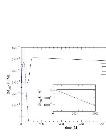
Figure 16: Accretion of a scalar wave packet across a Cauchy–peturbative matching interface. To demonstrate the advantage of using high-order methods, $(M_{AH}-1)$ is shown for evolutions obtained with the SBP operators $D_{4-3}$ $D_{6-5}$, with resolution $\Delta r=M/10$. The loss of mass after accretion of the wave packet with compact support in $t\in[0,100]M$ is a numerical artefact, which converges away with resolution. The inset shows that the evolution obtained with the operator $D_{4-3}$ is not unstable, but only significantly less accurate.

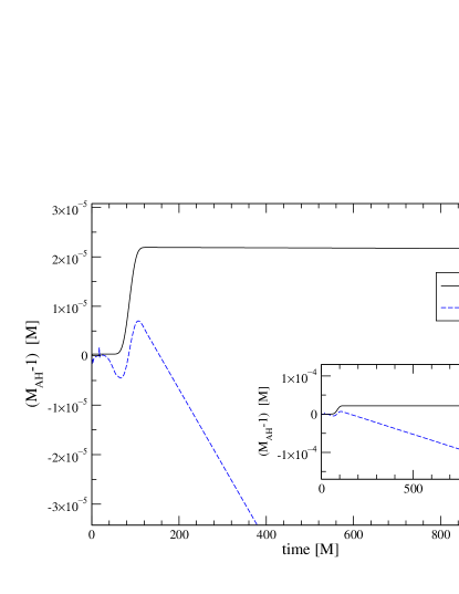
Figure 17: Like figure 16, but for a resolution of $\Delta r=M/20$.

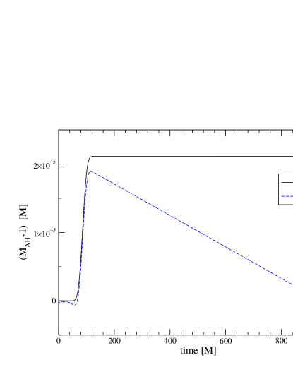
Figure 18: Like Figure 16, but for a resolution of $\Delta r=M/40$.

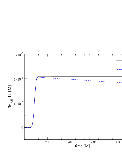
Figure 19: Like Figure 16, but for a resolution of $\Delta r=M/80$.

The advantages of using high-order methods is made evident in Figures 16, 17, 18, and 19. In these plots, the performance of the SBP operator $D_{6-5}$, which is sixth order in the interior and fifth order at the boundaries, is compared to that of the operator $D_{4-3}$, which is fourth order in the interior and third order at the boundaries, for different choices of resolution. Although both operators show convergence, for a mass increase of about $10^{-5}$, the operator $D_{4-3}$ is unable to reproduce the correct behaviour with reasonable grid resolutions. We consider this specifically important for three-dimensional simulations, where the necessary resources scale with $n^{4}$ if $n$ denotes the number of grid points in each direction. Thus, for all simulations requiring a certain amount of precision, high-order operators are an essential requirement.

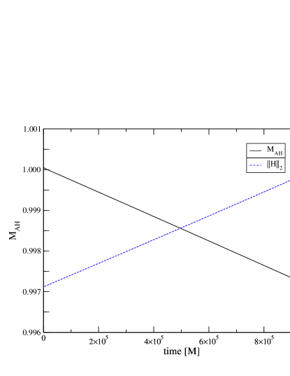
Figure 20: Long-term stable evolution of a Schwarzschild black hole after accretion of a scalar wave packet with Cauchy–perturbative matching. The SBP operator $D_{6-5}$ is used with a resolution of $\Delta r=M/10$. Plotted are the apparent horizon mass and the Hamiltonian constraint over time. The apparent horizon mass indicates that the discrete evolution introduces a relative error of about $0.3\%$ after $1,000,000M$.

The long-term evolution of a Schwarzschild black hole accreting a wave packet over a Cauchy–perturbative matching interface and settling down to equilibrium is shown in Figure 20. The black hole is evolved for $1,000,000M$ with the lowest resolution $\Delta r=M/10$ and the SBP operator $D_{6-5}$. While an evolution of this length might appear to be of only technical interest, we note that modelling phenomena like hypernovae and collapsars in general relativity will require the stable evolution of a black hole for at least several seconds, which is the lower end of timescales associated with the collapsar model of gamma-ray burst engines MacFadyen et al. (2001). For a stellar mass black hole, $M=M_{\odot}\approx 5\mu s$, that is $1s\approx 200,000M_{\odot}$.

IV Conclusions and outlook

To obtain long-term evolutions of compact astrophysical systems in three spatial dimensions, advanced numerical techniques are preferable in that they may improve stability and accuracy of the associated discrete model system. While high accuracy enables efficient use of the available computational resources, well-posedness of the continuum model and numerical stability are requirements which can not be met by increasing computational power. A number of techniques has been suggested to address these issues Lehner et al. (2005b): Multiple coordinate patches, typically adapted to approximate symmetries of certain solution domains, combined with high-order operators are expected to increase the accuracy of any model of a stellar system. Cauchy–perturbative matching provides an efficient way to accurately model the propagation of gravitational waves to a distant observer, and to yield physical boundary conditions on incoming modes of the Cauchy evolution. Constraint-preserving boundary conditions isolate the incoming modes on the constraint hypersurface, and, finally, for evolving black holes, an excision boundary is desirable to concentrate on the behaviour of the external spacetime. Only recently the consideration of the well-posedness of the differential system and the application of theorems on discrete stability of the numerical system have provided hints as how to address the outstanding issues. In this paper, we have applied all these techniques to a model system: a spherically symmetric black hole coupled to a massless Klein-Gordon field.

We find that the use of a first-order hyperbolic formulation of Einstein’s field equations, combined with high-order derivative and dissipation operators with the summation-by-parts property, penalized inter-patch boundary conditions and constraint-preserving outer boundary conditions leads to a stable and accurate discrete model. Specifically, isolated Schwarzschild black holes in coordinates adapted to the Killing fields, and in coordinates on which a gauge wave is imposed, and Schwarzschild black holes accreting scalar wave pulses were taken as typical model systems involving excision. The results show that the introduction of several coordinate patches and of a Cauchy–perturbative matching interface does not introduce significant artefacts or instabilities. Rather, the high-order methods allow the accurate long-term evolution of accreting black holes with excision and Cauchy–perturbative matching in reasonable resolutions. As an example, we have presented the evolution of such a system with the high-order SBP operator $D_{6-5}$, which, at a resolution of $\Delta x=M/10$, introduced an error of only $0.3\%$ after an evolution time of $1,000,000M$.

Most system of interest in general relativistic astrophysics will necessarily require the use of three-dimensional codes. Results from a one-dimensional study are useful in that they (i) allow to gain experience in a clean but non-trivial physical system, (ii) can be easily reproduced without the need to implement three-dimensional codes with multiple coordinate patches and (iii) allow to isolate sources of difficulty in the three-dimensional setting more easily. With the promising results from this study, we will, as a next step, apply these techniques to a three-dimensional, general relativistic setting.