Metric of a tidally perturbed spinning black hole

Abstract

We explicitly construct the metric of a Kerr black hole that is tidally perturbed by the external universe in the slow-motion approximation. This approximation assumes that the external universe changes slowly relative to the rotation rate of the hole, thus allowing the parameterization of the Newman-Penrose scalar $\psi_{0}$ by time-dependent electric and magnetic tidal tensors. This approximation, however, does not constrain how big the spin of the background hole can be and, in principle, the perturbed metric can model rapidly spinning holes. We first generate a potential by acting with a differential operator on $\psi_{0}$. From this potential we arrive at the metric perturbation by use of the Chrzanowski procedure in the ingoing radiation gauge. We provide explicit analytic formulae for this metric perturbation in Kerr coordinates, where the perturbation is finite at the horizon. This perturbation is parametrized by the mass and Kerr spin parameter of the background hole together with the electric and magnetic tidal tensors that describe the time evolution of the perturbation produced by the external universe. In order to make the metric accurate far away from the hole, these tidal tensors should be determined by asymptotically matching this metric to another one valid far from the hole. The tidally perturbed metric constructed here could be useful in initial data constructions to describe the metric near the horizons of a binary system of spinning holes. This perturbed metric could also be used to construct waveforms and study the absorption of mass and angular momentum by a Kerr black hole when external processes generate gravitational radiation.

I Introduction

Gravitational wave observatories, such as LIGO and VIRGO, have the potential to study black holes in the strong field regime Cutler and Thorne (2002). These black holes are expected to be immersed in a sea of gravitational perturbations that will alter the gravitational field of the background hole. Even though tidal perturbations are expected to be small relative to the background, they will be important in some astrophysical scenarios when attempting to provide an accurate description of the non-linear dynamical orbital evolution of bodies around this background. The need for high accuracy in the description of the orbital evolution derives from the fact that gravitational wave observatories are extremely sensitive to the phase of the gravitational waves emitted by the system. Therefore, since this phase is directly related to the orbital evolution, in some astrophysical scenarios it is necessary to take these tidal effects into consideration.

The study of gravitational perturbations around Kerr black holes is important for several reasons. First, it is of astrophysical interest to study the flux of mass and angular momentum across a perturbed Kerr horizon Poisson (2004a); Poisson and Sasaki (1995); Tagoshi et al. (1997); Alvi (2001), which can be calculated through manipulations of the tidally perturbed metric computed in this paper. Although this flux might be small for equal-mass binaries, in extreme-mass ratio inspirals (EMRI) up to $5\%$ of the total energy might be absorbed by the background hole. This absorption might slow down the orbital evolution increasing the duration of the gravitational wave signal Martel (2004); Hughes (2001). Space-based detectors, such as LISA, will be able to observe and measure the gravitational waveforms of EMRIs, since they have particularly low noise in the low frequency band where such inspirals are common. Therefore, precise knowledge of the gravitational waveform including the tidal perturbations effects might be important in data analysis Glampedakis and Babak (2005). Finally, the explicit formulae of this paper might be useful to compute initial data near the horizons of a binary system of spinning holes. For example, Refs. Alvi (2000); Yunes et al. (2005) make use of such explicit formulae for the non-spinning case to construct initial data via asymptotic matching. This data might be useful to the numerical relativity community because it derives from an approximate solution to the Einstein equation and, thus, we expect it to accurately describe the gravitational field of the system up to uncontrolled remainders.

In this paper, we analytically construct explicit formulae for the metric of a tidally perturbed Kerr hole, where the perturbations of the external universe are assumed to vary slowly in a well-defined sense. Metric perturbations for non-spinning holes have been studied in Refs. D’Eath (1975a, b, 1996); Alvi (2000); Poisson (2005) using the Regge-Wheeler formalism Regge and Wheeler (1957). However, this method is difficult to implement for spinning holes because the metric will now depend on both radius and angle $\theta$ in a non-trivial way, rendering the Einstein equations very difficult to solve. For this reason, we use the Chrzanowski procedure Chrzanowski (1975); Ori (2003) to construct the metric perturbation from the Newman-Penrose (NP) scalar $\psi_{0}$. This procedure allows us to calculate the metric in the so-called ingoing radiation gauge (IRG), which is suitable to study gravitational perturbations near the outer horizon ($r_{+}$), since there the metric is transverse and traceless.

We will work in the slow-motion approximation, described in detail in Refs. Burke and Thorne (1970); Burke (1971); D’Eath (1975a, b); Thorne and Hartle (1985); D’Eath (1996); Poisson (2004a, 2005), where we assume that the rate of change of the curvature of the external universe is small relative to the rotation rate of the background black hole, which in principle could be extremal. The external universe is completely arbitrary in that sense, as long as it respects the slow-motion approximation. For example, in the case where the external universe is given by a second black hole in a quasicircular orbit around the background hole, this approximation is valid as long as their orbital separation is sufficiently large. In particular, this separation must be at least greater than the inner most stable circular orbit (ISCO)Baumgarte (2000); Grandclement et al. (2002), so that the binary is still in a quasicircular orbit. In that case, the curvature generated by the second hole would correspond to the external universe, which will change slowly as long as the orbital velocity is sufficiently small. In this sense, the slow-motion approximation will hold for astrophysically realistic binaries as long as they are sufficiently separated.

Assuming this approximation to be valid, Poisson Poisson (2004a) has computed $\psi_{0}$ in the neighborhood of a spinning hole. First, the Weyl tensor of the spacetime is re-expressed in terms of the electric and magnetic tidal tensors of the external universe. Using the slow-motion approximation, Poisson argues that these tensors will be spatially coordinate independent if evaluated at sufficiently large distances from the worldline of the hole. With this tensor, the asymptotic form of $\psi_{0}$, denoted by $\tilde{\psi}_{0}$, is computed far from the hole by projecting the Weyl tensor onto the Kinnersly tetrad. This scalar will be a combination of slowly varying functions of time, which will be parametrized via the electric and magnetic tidal tensors, and scalar functions of the spatial coordinates, which will be given by the tetrad. The asymptotic form of $\psi_{0}$ now allows for the construction of an ansatz for $\psi_{0}$, which consists of its asymptotic form $\tilde{\psi}_{0}$ multiplied by a set of undetermined function of radius $R_{m}(r)$. These functions must satisfy the asymptotic condition $R_{m}\to 1$ as $r\gg r_{+}$, as well as the Teukolsky equation. This last condition is a differential constraint on $R_{m}(r)$ which can be solved for explicitly, thus allowing for the full determination of $\psi_{0}$. In this manner, the final expression for $\psi_{0}$ is obtained and is now valid close to the horizon as well, in particular, approaching the perturbations generated by the external universe sufficiently far from the hole’s worldline.

Once $\psi_{0}$ has been calculated, we can apply the Chrzanowski procedure to compute the metric perturbation, still in the slow-motion approximation. This calculation contains two parts: the computation of a potential ($\Psi$) and the determination of the metric perturbation ($h_{ab}$) from $\Psi$. In principle, one might think that it would be easier to try to compute $h_{ab}$ directly from $\psi_{0}$. Chrzanowski Chrzanowski (1975) attempted this by applying a differential operator onto $\psi_{0}$. However, Wald Wald (1978) discovered that doing this leads to a physically different gravitational perturbation from that represented by $\psi_{0}$. Cohen and Kegeles Kegeles and Cohen (1979) showed that by constructing a Hertz-like potential $\Psi$ from $\psi_{0}$ first and then applying Chrzanowski’s differential operator to $\Psi$ instead leads to the real metric perturbation. This is the procedure we will follow to construct the metric perturbation in this paper.

The construction of $\Psi$ requires the action of a fourth order differential operator on $\psi_{0}$, where here we follow Ori Ori (2003). This potential is simplified by the use of the slow-motion approximation that allows us to neglect any time derivatives of the electric and magnetic tidal tensors. Once $\Psi$ is calculated, we can apply Chrzanowski’s differential operator to this potential Kegeles and Cohen (1979); Campanelli and Lousto (1999). In this manner, we compute the metric of a perturbed spinning hole from a tidal perturbation described by $\psi_{0}$ in terms of tidal tensors. These tensors are unknown functions of time that represent the external universe and which should be determined by asymptotically matching this metric to another approximation valid far from the holes Alvi (2000); Yunes et al. (2005).

The metric computed here, however, has a limited applicability given by the validity of the slow-motion approximation and the Chrzanowski procedure. The slow-motion approximation implies that we can neglect all derivatives of the tidal tensors. Furthermore, since we are working only to first non-vanishing order in this approximation, it suffices to consider only the quadrupolar perturbation of the metric, since the monopolar and dipolar perturbations are identically zero. In perturbation theory, any $l$ mode in the decomposition of the perturbation is one order larger than the $l+1$ mode. Therefore, any higher modes or couplings of the quadrupole to other modes will be of higher order. The Chrzanowski procedure also possesses a limited region of validity, given by a region sufficiently close to the event horizon so that the spatial distance from the horizon to the radius of curvature of the external universe is small. This restriction is because the Chrzanowski procedure builds the metric as a linear perturbation of the background and neglects any non-linear interactions with the external universe. In particular, this restriction implies that this metric cannot provide valid information on the dynamics of the entire spacetime. However, if this metric is asymptotically matched to another approximation that is valid far from the background hole, then the combined global metric will describe the the $3$-manifold accurately.

We verify the validity of our calculations in several ways. First, we check that $\psi_{0}$ indeed satisfies the Teukolsky equation. After computing $\Psi$, we also check that it satisfies the Teukolsky equation and the differential constraint that relates $\Psi$ to $\psi_{0}$. Finally, we check that the metric perturbation constructed with this potential satisfies all of the Einstein equations to the given order. We further check that this perturbation is indeed transverse and traceless in the tetrad frame so that it is suitable for the study of gravitational perturbations near the horizon.

This paper is divided as follows. Sec. II describes the slow-motion approximation in detail, summarizes some relevant results from Ref. Poisson (2004a) and establishes some notation. Sec. III computes $\Psi$ from $\psi_{0}$ while Sec. IV calculates $h_{ab}$ from $\Psi$. Finally, Sec. V presents some conclusions and points toward future work. In the appendix, we provide an explicit transformation to Kerr-Schild coordinates that might be more amenable to numerical implementation.

In the remaining of the paper, we use geometrized units ($G=1$, $c=1$) and the symbol $O(a)$ stands for terms of order $a$, where $a$ is dimensionless. Latin indices range from $0$ to $3$, where $0$ is the time coordinate. The Einstein summation convention is assumed all throughout the paper, where repeated indices are to be summed over unless otherwise specified. Tetrad notation will be used, where indices with parenthesis refer to the tetrad and those without parenthesis to the components of the tensor. The relational symbol $\sim$ stands for “asymptotic to” as defined in Bender and Orszag (1999), while the symbols $\ll$ and $\gg$ are also to be understood in the asymptotic sense. In particular, note that if $f(r)$ is valid for $r\ll b$, then this function is not valid as $r\to b$. In this paper we have relied heavily on the use of symbolic manipulation software, such as MAPLE and MATHEMATICA.

II The slow-motion approximation and the NP scalar

In this section we will describe the slow-motion approximation in more detail and discuss the construction of $\psi_{0}$ due to perturbations of the external universe. Both the slow-motion approximation and $\psi_{0}$ have already been explained in detail and computed by Poisson in Ref. Poisson (2004a). Therefore, here we follow this reference and summarize the most relevant results for this paper while establishing some notation.

Let us begin by discussing the slow-motion approximation. Consider a non-spinning black hole of mass $m_{1}$ immersed in an external universe, with radius of curvature ${\cal{R}}$. This external universe could be given by any object that lives in the exterior of the hole’s horizon, such as a scalar field or another black hole. The slow-motion approximation requires that the external universe’s length scales be much larger than the hole’s scales. In other words, for the non-spinning case we must have $m_{1}/{\cal{R}}\ll 1$, since these are the only scales available.

For concreteness, let us assume that the external universe can be described by another object of mass $M_{ext}$ and that our hole is in a quasicircular orbit around it. Then, we have

$$\frac{m_{1}}{{\cal{R}}}\sim\frac{m_{1}}{m_{1}+M_{ext}}V^{2},\qquad V=\sqrt{\frac{m_{1}+M_{ext}}{b}},$$ (1)

where $V$ is the orbital velocity and $b$ is the orbital separation. There are two ways of enforcing $m_{1}/{\cal{R}}\ll 1$: the small-body approximation, where we let $m_{1}/M_{ext}\ll 1$; and the slow-motion approximation, where $V\ll 1$. However, in a future paper we might want to asymptotically match the metric perturbation computed in this paper to a post-Newtonian (PN) expansion Blanchet (2002), which requires small velocities. For this reason, we will restrict our attention to the slow-motion approximation, which implies that we can only investigate systems that are sufficiently separated. The ISCO is not a well-defined concept for black hole binaries, but it has been estimated for non-spinning binary numerically Baumgarte (2000); Grandclement et al. (2002) to be given approximately by $\omega_{ISCO}M/10$, where $M$ and $\omega_{ISCO}$ are the total mass of the system and its angular velocity at the ISCO respectively. For spinning binaries the holes can get closer without plunging, where the value of the ISCO becomes a function of the spin parameter of the holes. Regardless of the type of binary system, the slow-motion approximation will hold as long as we consider systems that are separated by at least more than their ISCO so that they are still in a quasicircular orbit.

The above considerations suffice for non-spinning holes because there is only one length scale associated with it, $m_{1}$. However, for spinning ones we must also take into account the time scale associated with the intrinsic spin of the hole. The slow motion approximation does not constraint how large the spin of the background hole could be. However, in the standard theory, it is usually assumed that isolated holes will obey $a<m_{1}$, where $a$ is the rotation parameter of the hole and $m_{1}$ is its mass. If the previous inequality did not hold, then the hole would be tidally disrupted by centrifugal forces. When the background hole is surrounded by an accretion disk, however, some configuration might lead to a violation of the previous condition Ansorg and Petroff (2005), but we will not consider those in this paper. Let us then define a dimensionless rotation parameter $\chi=a/m_{1}$, which is now restricted to $0<\chi<1$. The mass of the hole and this rotation parameter now define a new timescale, related to the rotation rate of the horizon and given by

$$\tau_{H}=\frac{1}{\Omega_{H}}=\frac{2m_{1}}{\chi}(1+\sqrt{1-\chi^{2}}),$$ (2)

where $\Omega_{H}$ is the angular velocity of the hole’s horizon Poisson (2004b). The slow-motion approximation then requires this time scale to be much smaller than the time scale associated with the change of the radius of curvature of the external universe, $\tau_{ext}$, i.e. $\tau_{H}/\tau_{ext}\ll 1$. This condition then becomes

$$m_{1}/{\cal{R}}\ll\chi,$$ (3)

since $\tau_{ext}\approx{\cal{R}}$. We take the above relation as the precise definition of the slow-motion approximation for spinning black holes. Following the reasoning that lead to Eq. (1), we must then have $V^{2}\ll\chi$, which, for a binary system, means that the orbital velocity of the system cannot exceed the rotation rate of the background hole. Thus, the slow-motion approximation implies that, to this order and for spinning holes, we can also only consider systems that are sufficiently separated and where the black holes have relatively rapid spins. This reasoning does not imply that the Schwarzschild limit is incompatible with the slow motion approximation. Actually, Poisson Poisson (2004a) showed that when computing certain quantities, such as $\psi_{0}$, this limit can be recovered if we work to higher order in the slow-motion approximation. The precise radius of convergence of the slow-motion approximation to first order remains unknown, but an approximate measure of how small a separation the approximation can tolerate will be studied in a later section.

Now that the slow-motion approximation has been explained in detail, let us proceed with the construction of $\psi_{0}$, which is defined by

$$\psi_{0}=C_{abcd}l^{a}m^{b}l^{c}m^{d},$$ (4)

where $C_{abcd}$ is the Weyl tensor of the spacetime and $l^{a}$ and $m^{a}$ are the first and third tetrad vectors. This null vector $m^{a}$ is not to be confused with the $m$ that we will introduce later in this section to denote the angular mode of the perturbation. Poisson works with the Kinnersly tetrad in advanced Eddington-Finkelstein (EF) coordinates, also known as Kerr coordinates, which are well-behaved at the outer horizon, given by $r_{+}=m_{1}+(m_{1}^{2}-a^{2})^{1/2}$.

The calculation of $\psi_{0}$ is based on making an ansatz guided by its asymptotic form far from the worldline of the hole but less than the radius of curvature of the external universe, i.e. $r_{+}\ll r\ll{\cal{R}}$. In this region, the Weyl tensor can be decomposed into electric ${\cal{E}}_{ab}$ and magnetic ${\cal{B}}_{ab}$ tidal fields, which are slowly varying functions of advanced time $v$ only. Thus, in this region, the only spatial coordinate dependence in $\psi_{0}$ is given by the tetrad, namely

$$\tilde{\psi}_{0}\sim-\sum_{m}z_{m}(v)\;_{2}Y_{2}^{m}(\theta,\phi),$$ (5)

where the tilde is to remind us that this quantity is the asymptotic form of $\psi_{0}$ and where ${}_{2}Y_{2}^{m}(\theta,\phi)$ are spin-weighted spherical harmonics, given by

$${}_{2}Y^{0}_{2}(\theta,\phi) = -\frac{3}{2}\sin^{2}{\theta},$$

$${}_{2}Y^{\pm 1}_{2}(\theta,\phi) = -\sin{\theta}(\cos{\theta}\mp 1)e^{\pm i\phi},$$

$${}_{2}Y^{\pm 2}_{2}(\theta,\phi) = \frac{1}{4}(1\mp 2\cos{\theta}+\cos^{2}{\theta})e^{\pm 2i\phi}.$$ (6)

In Eq. (5), the quantities $z_{m}(v)$ are complex combinations of the tidal fields given by $z_{m}(v)=\alpha_{m}(v)+i\beta_{m}(v)$, where

$$\alpha_{0}(v) = {\cal{E}}_{11}(v)+{\cal{E}}_{22}(v),$$

$$\alpha_{\pm 1}(v) = {\cal{E}}_{13}(v)\mp i{\cal{E}}_{23}(v),$$

$$\alpha_{\pm 2}(v) = {\cal{E}}_{11}(v)-{\cal{E}}_{22}(v)\mp 2i{\cal{E}}_{12}(v),$$

$$\beta_{0}(v) = {\cal{B}}_{11}(v)+{\cal{B}}_{22}(v),$$

$$\beta_{\pm 1}(v) = {\cal{B}}_{13}(v)\mp i{\cal{B}}_{23}(v),$$

$$\beta_{\pm 2}(v) = {\cal{B}}_{11}(v)-{\cal{B}}_{22}(v)\mp 2i{\cal{B}}_{12}(v).$$ (7)

Note that in this region, $\psi_{0}$ is independent of radial coordinate.

With Eq. (5) at hand, Poisson makes an ansatz for the functional form of $\psi_{0}$, namely

$$\psi_{0}=-\sum_{m}z_{m}(v)R_{m}(r)_{2}Y^{m}_{2}(\theta,\phi),$$ (8)

where $R_{m}(r)$ is an undetermined function of radius that must satisfy $R_{m}(r)\to 1$ as $r\gg r_{+}$. If Eq. (8) is inserted into the Teukolsky equation, one obtains a differential equation for $R_{m}(r)$. The angular part of the Teukolsky equation is automatically satisfied by the angular decomposition of $\psi_{0}$ in spin-weighted spherical harmonics with eigenvalue $E=4$ (Eq. $2.10$ in Ref. Press and Teukolsky (1973)). The spatial part of the Teukolsky equation yields a differential constraint for $R_{m}(r)$ namely,

$$\left\{x(1+x)\frac{d^{2}}{dx^{2}}\right. +\left.\left[3(2x+1)+2im\gamma\right]\frac{d}{dx}\right.$$ (9)

$$\left.+4im\gamma\frac{2x+1}{x(1+x)}\right\}R_{m}(x)=0,$$

where $x$ is a rescaled version of the radial coordinate given by

$$x=\frac{r-r_{+}}{r_{+}-r_{-}},$$ (10)

and where the inner and outer horizons are given, respectively, by $r_{\pm}=m_{1}^{2}\pm(m_{1}^{2}-a^{2})^{1/2}$. We should note that $r_{+}$ is an event horizon, while $r_{-}$ is actually an apparent horizon. Solving this equation Poisson (2004a) one obtains

$$R_{m}(r)=A_{m}x^{-2}(1+x)^{-2}F(-4,1,-1+2im\gamma;-x),$$ (11)

where $A_{m}$ is a normalization constant given by

$$A_{m}=-\frac{i}{6}m\gamma(1+im\gamma)(1+4m^{2}\gamma^{2}).$$ (12)

In Eq. (11), the function $F(a,b,c;x)$ is the hypergeometric function

$$F(a,b,c;x)=\sum_{n=0}^{\infty}\frac{(a)_{n}(b)_{n}}{(c)_{n}}\frac{x^{n}}{n!},$$ (13)

where $(a)_{n}$ is the Pochammer symbol defined as

$$(a)_{n} = a(a+1)(a+2)\ldots(a+n-1)=\frac{(a+n-1)!}{(a-1)!},$$

$$(a)_{0} = 1.$$ (14)

For the present case, the series gets truncated at the fourth power and we obtain

$$F(-4,1,-1+2im\gamma;-x)=\left(1+\frac{4}{2im\gamma-1}x\right.$$

$$\left.+\frac{6}{(2im\gamma-1)im\gamma}x^{2}+\frac{12}{(2im\gamma-1)im\gamma(2im\gamma+1)}x^{3}\right.$$

$$\left.+\frac{12}{(2im\gamma-1)im\gamma(2im\gamma+1)(2im\gamma+2)}x^{4}\right),$$ (15)

where $\gamma$ is a constant given by

$$\gamma=\frac{a}{r_{+}-r_{-}}.$$ (16)

In this manner, Poisson calculates $\psi_{0}$, which encodes the gravitational perturbations of the external universe on a spinning hole in the slow-motion approximation. The full expression for $\psi_{0}$ is then given by

$$\psi_{0}=-\sum_{m\neq 0}B_{m}x^{-2}(1+x)^{-2} \left(1+\frac{4}{2im\gamma-1}x+\frac{6}{(2im\gamma-1)im\gamma}x^{2}+\frac{12}{(2im\gamma-1)im\gamma(2im\gamma+1)}x^{3}\right.$$ (17)

$$\left.+\frac{12}{(2im\gamma-1)im\gamma(2im\gamma+1)(2im\gamma+2)}x^{4}\right)\;_{2}Y^{m}_{2}(\theta,\phi),$$

where we have used the final abbreviation

$$B_{m}=A_{m}z_{m}(v),$$ (18)

without summing over repeated indices here, to group all terms that are spatially coordinate independent. We have checked that Eq. (17) indeed satisfies the Teukolsky equation Press and Teukolsky (1973) for the $s=2$ mode that corresponds to this scalar. Note that, in this final expression, summation over the $m=0$ mode is removed because Poisson Poisson (2004a) has shown that it corresponds to the Schwarzschild limit and, thus, it contributes at a relative $O(m_{1}/{\cal{R}})$ higher than all other modes. Also note that the final expression for $\psi_{0}$ only contains the quadrupolar $l=2$ mode, once more because higher multipoles will be smaller by a relative factor of $m_{1}/{\cal{R}}$ in the slow-motion approximation. For this reason, there are no mode couplings in the $\psi_{0}$ presented above.

The time-evolution of the tidal perturbation will be exclusively governed by the electric and magnetic tidal fields. These tensors should be determined by asymptotically matching the metric perturbation generated by this $\psi_{0}$ to another approximation valid far from the hole. However, in Refs. Thorne and Hartle (1985); Alvi (2000); Yunes et al. (2005); Poisson (2005) it has been shown that when the external universe is given by another non-spinning black hole in a quasicircular orbit, these tensors scale approximately as

$$z_{m}\approx\frac{m_{2}}{b^{3}},$$ (19)

where $m_{2}$ is the mass of the other hole (the external universe) and $b$ is the orbital separation (approximately equal to the radius of curvature of the external universe). Note that the factor of $b^{3}$ in the denominator is necessary to make the tidal tensors dimensionally correct. Also note that in Eq. (19) we have neglected the time dependence of the tidal fields, which generally is given by a trigonometric function, since we are interested in a spatial hypersurface of constant time. For the case where the other hole is spinning, Eq. (19) will contain corrections proportional to $\chi$, but these terms will not change the overall scale of the tidal tensors.

Throughout the rest of the paper we will generate plots of physical quantities, such as $\psi_{0}$, $\Psi$ and $h_{ab}$. For the purpose of plotting, we will have to make two choices: one regarding the physical scenario that produces the perturbation of the external universe; and another regarding the parameters of the background black hole. As for the physical scenario, we will choose the external universe to be given by another orbiting black hole in a quasicircular orbit. This choice allows us to represent the tidal fields with the scaling given in Eq. (19). This scaling is not the exact functional form of the tidal fields and, therefore, the plots generated will not be exact. However, this scaling will allow us to provide plots accurate enough to study the general features of the global structure of the quantities plotted, as well as some local features near the horizons. Regarding the parameter choice, we will assume $m_{1}=m_{2}$, $a=0.99m_{1}$, and $b=10m_{1}$, where $M=m_{1}+m_{2}=1$ is the total mass. These choices are made in accordance with the slow-motion approximation, while making sure the system is not inside its ISCO. However, the formulae presented in this paper should apply to other choices of physical scenarios and background parameters as well, as long as these do not conflict with the slow motion approximation.

Given the chosen physical scenario, the formulae in this paper should apply to other mass ratios and separations, as long as the orbital velocity does not become too large. For the background parameters chosen, the orbital velocity is approximately $V\approx 0.3$, which indicates that, for fixed masses, we cannot reduce the orbital separation by much more without breaking the slow-motion approximation. However, since we provide explicit analytic formulae for all relevant physical quantities, we can estimate their error by considering the uncontrolled remainders, i.e.  the neglected terms in the approximation. In particular, in a later section, we will see that the uncontrolled remainders are still much smaller than the perturbation itself even at $b=10M$ as long as we restrict ourselves to field points sufficiently near the outer horizon of the background hole.

In Fig.1 we plot the real part of $\psi_{0}$ with the plotting choices described earlier.

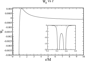
Figure 1: Plot of the real part of the NP scalar $\psi_{0}$ along the $x$-axis with the plotting parameters described in Sec. II.

Observe that as $r$ becomes large the scalar asymptotes to a constant given by ${\tilde{\psi}}_{0}$. Also observe that the functional behavior of the scalar is drastically different as $r$ becomes small. In this figure, as well as in future figures, we have chosen to include an inset where we zoom to a region close to the horizons, so that we can observe its local and global behavior. For the orbital parameter chosen, the inner and outer horizons are given by $r_{-}\approx 0.43M$ and $r_{+}\approx 0.57M$. Observe from the inset in Fig. 1 that the scalar diverges at the horizons and as $r\to 0$, which is due to the choice of tetrad. Finally, observe that, except for where it diverges, the real part of $\psi_{0}$ is of $O(V^{2})$ in the entire $3$-manifold.

III The potential

In this section we will use $\psi_{0}$ to construct the potential $\Psi$ by acting some differential operators on the NP scalar. This potential must satisfy the vacuum Teukolsky equation for the $s=-2$ mode together with the differential equation

$$\psi_{0}=D^{4}[\bar{\Psi}],$$ (20)

where the overbar stands for complex conjugation and where the differential operator is given by $D=l^{a}\partial_{a}$ Wald (1978); Lousto and Whiting (2002); Ori (2003).

Ori Ori (2003) has shown that the above differential equations can be inverted with use of the Teukolsky-Starobinsky relation to obtain

$$\Psi=\frac{1}{p}\Delta^{2}(D^{{\dagger}})^{4}[\Delta^{2}\bar{\psi}_{0}],$$ (21)

where here $\Delta$ is given by

$$\Delta=r^{2}-2m_{1}r+a^{2},$$ (22)

while $p$ is a constant that for the time-independent case reduces to

$$p=\left[l(l+1)-s^{2}+|s|\right]^{2}\left[l(l+1)-s^{2}+|s|+2\right]^{2}.$$ (23)

In our case, since $s$ and $l$ refer to $\psi_{0}$, $s=2$ and $l=2$ so that this constant becomes $p=576$.

The differential operator $D^{{\dagger}}$ is given in spherical Brill-Lindquist (BL) coordinates $(t_{BL},r,\theta,\phi_{BL})$ by

$$D^{{\dagger}}_{BL}=\partial_{r}-\frac{a}{\Delta}\partial_{\phi_{BL}},$$ (24)

neglecting any time dependence, since time derivatives will only contribute at a higher order. In order to compute $\Psi$ in Kerr coordinates, we must transform the above differential operator. The transformation between Kerr and BL coordinates is given by

$$dv = dt_{BL}+dr_{BL}\left(\frac{2m_{1}r}{\Delta}+1\right),$$

$$dr = dr_{BL},$$

$$d\theta = d\theta_{BL},$$

$$d\phi = d\phi_{BL}+dr_{BL}\frac{a}{\Delta}.$$ (25)

After transforming the differential operator $D^{{\dagger}}_{BL}$ we obtain

$$D^{{\dagger}}=\partial_{r},$$ (26)

because the $dr_{BL}/d\phi$ term in the transformation cancels the $\phi$ dependence. Note that $r$ and $\theta$ do not change in this transformation and, thus, $\Delta$ remains unchanged. Also note that $\Psi$ is a scalar constructed from differential operators on $\psi_{0}$ and, since the latter is a scalar, $\Psi$ will also be gauge invariant.

Before plugging in Eq. (17) into Eq. (21) to compute $\Psi$, let us try to simplify these expressions. In the previous section, we defined the inner and outer horizons $r_{+}$ and $r_{-}$, as well as the new variable $x$. We can invert the definition of $x$ so that it becomes a definition for $r$ as a function of $x$ and then insert this into Eq. (22). We then obtain

$$\Delta=4\eta x(1+x),$$ (27)

where we have defined $\eta=m_{1}^{2}-a^{2}$. It is clear now that when we combine the square of this expression with Eq. (17) some cancellations will occur that will simplify all future calculations.

We are now ready to compute $\Psi$, but first let us rewrite the function we want to differentiate, namely

$$\Delta^{2}\bar{\psi}_{0}=\sum_{m\neq 0}\bar{C}_{m}\bar{F}(x)\;_{2}{\bar{Y}}_{2}^{m}(\theta,\phi_{BL}),$$ (28)

where $F(x)$ is shorthand for the aforementioned hypergeometric function and where $C_{m}$ is a new function of advanced time only given by

$$C_{m}=-16B_{m}\eta^{2}=-16A_{m}\eta^{2}z_{m}(v).$$ (29)

Note that the angular dependence occurs in the spherical harmonics, while the only $x$ dependence is in the hypergeometric function. We can transform the $D^{{\dagger}}$ operator to $x$ space to obtain

$$D^{{\dagger}}=\partial_{r}=\frac{1}{2\eta^{1/2}}\partial_{x}.$$ (30)

Applying all these simplifications, $\Psi$ becomes

$$\Psi=\frac{\Delta^{2}}{576}\sum_{m\neq 0}\bar{C}_{m}\;{}_{2}{\bar{Y}}_{2}^{m}(\theta,\phi)\frac{1}{16\eta^{2}}\partial_{x}^{4}[\bar{F}(x)].$$ (31)

We can now apply all derivatives to obtain

$$\Psi=\frac{\Delta^{2}}{576}\sum_{m\neq 0}\bar{C}_{m}\;{}_{2}{\bar{Y}}_{2}^{m}(\theta,\phi)\frac{\bar{F}^{(4)}}{16\eta^{2}},$$ (32)

where we have used the shorthand $\bar{F}^{(n)}$ which stands for the $n$th derivative of the complex conjugate of the hypergeometric function. This derivative is given by

$$\bar{F}^{(4)}=\frac{288}{(2im\gamma+1)im\gamma(-2im\gamma+1)(-2im\gamma+2)},$$ (33)

Note that we can reexpress the constant $\gamma$ in terms of $\eta$ as $\gamma=a/(2\eta^{1/2})$. Interestingly this constant combines with $\bar{C}_{m}$ to return an overall constant that is purely real so that $\Psi$ is given by

$$\Psi=-\frac{1}{24}\Delta^{2}\sum_{m\neq 0}Y^{m}(\theta)e^{-im\phi}\bar{z}_{m}(v),$$ (34)

where here $Y^{m}$ stands for the $l=2$ spherical harmonics with zero $\phi$ dependence. We have checked that the potential of Eq. (34) indeed satisfies the definition of Eq. (20) as well as the Teukolsky equation for the $s=-2$ mode with angular eigenvalue $E=10$. Note that $\Psi$ has units of mass squared because the electric and magnetic tidal fields scale as the inverse of the mass squared. Furthermore, note that eventhough $\psi_{0}$ is singular at the horizon, $\Psi$ is finite and actually vanishes there.

Next, we proceed to decompose $\Psi$ into real and imaginary parts. The potential contains $2$ complex terms, namely the $\phi$ part of the spherical harmonics and the electric and magnetic tidal tensors. Decomposing $\Psi$ we obtain

$$\Psi_{R} =-\frac{\Delta^{2}}{24}\sum_{m\neq 0}\;Y^{m}\left(\Re(z_{m})\cos{m\phi}-\Im(z_{m})\sin{m\phi}\right),$$

$$\Psi_{I} =+\frac{\Delta^{2}}{24}\sum_{m\neq 0}\;Y^{m}\left(\Re(z_{m})\sin{m\phi}+\Im(z_{m})\cos{m\phi}\right)\,,$$ (35)

where recall that $(\alpha_{m},\beta_{m})$ in $z_{m}$ are complex functions of $v$. Note that the entire radial dependence is encoded in $\Delta^{2}$, whereas the angular dependence is hidden in the spherical harmonics. The time dependence occurs only in the the tidal fields that should be determined via asymptotic matching, as mentioned previously. This is the potential in Kerr coordinates associated with the $\psi_{0}$ calculated in the previous section in the slow-motion approximation.

In Fig. 2 we plot $\Psi_{R}$ with the plotting choices described in Sec. II.

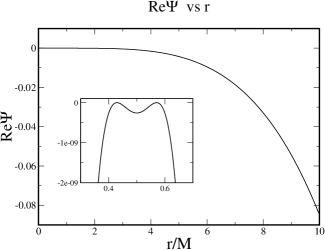
Figure 2: Plot of the potential $\Psi_{R}$ along the $x$-axis with the plotting parameters described in Sec. II.

Observe from the inset that the potential has nodes at both horizons. Also observe that the potential does not asymptote to a constant, but instead it grows quartically. This growth is due to the factor of $\Delta^{2}$ that dominates at large radius. Finally, note that the potential is still of $O(V^{2})$ for radii sufficiently close to the hole (roughly for $r<8m$).

IV The metric perturbation

In this section we compute the metric perturbation by applying Chrzanowski’s differential operator to the potential calculated in the previous section. The full metric of the spacetime is given by

$$g_{ab}=g^{B}_{ab}+h_{ab},$$ (36)

where $g^{B}_{ab}$ is the background metric and $h_{ab}$ is the perturbation. Since $\psi_{0}$ and $\Psi$ were computed in Kerr coordinates, the background should also be in this coordinate system. This background is given then by

$$g^{B}_{00} = -\left(1-\frac{2m_{1}r}{\Sigma}\right),$$

$$g^{B}_{01} = 1,$$

$$g^{B}_{03} = -\frac{m_{1}r}{\Sigma}(2a\sin^{2}{\theta}),$$

$$g^{B}_{13} = -a\sin^{2}{\theta},$$

$$g^{B}_{22} = \Sigma,$$

$$g^{B}_{33} = (r^{2}+a^{2})\sin^{2}{\theta}+\frac{2m_{1}r}{\Sigma}(a^{2}\sin^{4}{\theta}),$$ (37)

where $m_{1}$ is the mass of the background black hole, $a$ is its spin parameter, related to the angular momentum vector by $\vec{S}=m\vec{a}$, and where $\Sigma=r^{2}+a^{2}\cos^{2}{\theta}$.

Let us now construct the metric perturbation. We will work with the form of the differential operator presented in Ref. Campanelli and Lousto (1999), namely

$$h_{ab} = 2\Re\left(\left\{-l_{a}l_{b}(\delta+\bar{\alpha}+3\beta-\tau)(\delta+4\beta+3\tau)\right.\right.$$

$$\left.\left.-m_{a}m_{b}(D-\rho)(D+3\rho)+l_{(a}m_{b)}\left[(D-2i\rho_{I})\right.\right.\right.$$

$$\left.\left.\left.(\delta+4\beta+3\tau)+(\delta+3\beta-\bar{\alpha}-\bar{\pi}-\tau)\right.\right.\right.$$

$$\left.\left.\left.(D+3\rho)\right]\right\}\Psi\right),$$

where we have replaced $\bar{\rho}-\rho=-2i\rho_{I}$. The metric perturbation constructed in this fashion will be in the ingoing radiation gauge (IRG), which is defined by the conditions

$$h_{ll}=h_{ln}=h_{lm}=h_{l\bar{m}}=h_{m\bar{m}}=0.$$ (39)

In Eq. (IV) there are terms that depend on the differential operators $D=l^{a}\partial_{a}$ and $\delta=m^{a}\partial_{a}$, which in turn depends on the tetrad. To be consistent, we will continue to work with the Kinnersly tetrad in Kerr coordinates given by

$$e_{(1)}^{a} = l^{a}=\left(2\frac{r^{2}+a^{2}}{\Delta},1,0\frac{2a}{\Delta}\right),$$

$$e_{(2)}^{a} = n^{a}=\left(0,-\frac{\Delta}{2\Sigma},0,0\right).$$

$$e_{(3)}^{a} = m^{a}=\frac{1}{\sqrt{2}(r+ia\cos{\theta})}\left[ia\sin{\theta},0,1,\frac{i}{\sin{\theta}}\right],$$

$$e_{(4)}^{a} = \bar{m}^{a},$$ (40)

where the overbar stands for complex conjugation. Note that the $m^{a}$ vector is the same as the one in BL coordinates, but $l^{a}$ and $n^{a}$ are different. The differential operators associated with this tetrad in Kerr coordinates are

$$D = \partial_{r}+\frac{2a}{\Delta}\partial_{\phi}$$

$$\delta = \frac{1}{\sqrt{2}(r+ia\cos{\theta})}\left(\partial_{\theta}+\frac{i}{\sin{\theta}}\partial_{\phi}\right),$$ (41)

where once more we neglect the time derivatives by use of the slow motion approximation. The covariant form of the tetrad in these coordinates is given by

$$l_{a} = l_{a}^{R}=\left(1,-\frac{2\Sigma}{\Delta},0,-a\sin^{2}{\theta}\right),$$ (42)

$$n_{a} = n_{a}^{R}=\frac{1}{2\Sigma}\left(\Delta,0,0,-a\Delta\sin^{2}{\theta}\right),$$

$$m_{a}^{R} = \frac{a\sin{\theta}}{\sqrt{2}\Sigma}\left[a\cos{\theta},0,-\frac{r\Sigma}{a\sin{\theta}},-\cos{\theta}(r^{2}+a^{2})\right],$$

$$m_{a}^{I} = \frac{1}{\sqrt{2}\Sigma}\left[ar\sin{\theta},0,a\Sigma\cos{\theta},-r\sin{\theta}(r^{2}+a^{2})\right],$$

where the superscript $I$ and $R$ stand for the imaginary and real parts respectively. One can show that if this tetrad is used we can recover the background metric $g^{B}_{ab}$ with the formula $g^{B}_{ab}=2l_{(a}n_{b)}+2m_{(a}\bar{m}_{b)}$.

Eq. (IV) contains terms that depend on the spin coefficients of the background Chandrasekhar (2000). These coefficients, also called Ricci rotation coefficients for the case where the tetrad is non-null, are simply contraction of the tetrad with its derivatives. In the tetrad formalism, these quantities can also be related to the Riemann tensor. Let us decompose the spin coefficients into real and imaginary parts, i.e.

$$\rho_{R} = -\frac{r}{\Sigma},\qquad\rho_{I}=-\frac{a}{\Sigma}\cos{\theta},$$

$$\beta_{R} = \frac{\sqrt{2}}{4}\frac{r}{\Sigma}\cot{\theta},\qquad\beta_{I}=-\frac{\sqrt{2}}{4}\frac{a}{\Sigma}\cot{\theta}\cos{\theta},$$

$$\pi_{R} = -\sqrt{2}\frac{a^{2}}{\Sigma^{2}}r\sin{\theta}\cos{\theta},$$

$$\pi_{I} = \frac{\sqrt{2}}{2}\frac{a}{\Sigma^{2}}\left(r^{2}-a^{2}\cos^{2}{\theta}\right)\sin{\theta},\quad\tau_{I}=-\frac{\sqrt{2}}{2}\frac{a}{\Sigma}\sin{\theta},$$

$$\alpha_{R} = -\sqrt{2}\frac{a^{2}}{\Sigma^{2}}r\sin{\theta}\cos{\theta}-\frac{\sqrt{2}}{4}\frac{r}{\Sigma}\cot{\theta},$$

$$\alpha_{I} = \frac{\sqrt{2}}{2}\frac{a}{\Sigma^{2}}\sin{\theta}\left(r^{2}-a^{2}\cos^{2}{\theta}\right)-\frac{\sqrt{2}}{4}\frac{a}{\Sigma}\cot{\theta}\cos{\theta}.$$

These spin coefficients are the same as those obtained with the Kinnersly tetrad in BL coordinates. This invariance is due to the fact that the spin coefficients are only tetrad dependent but still gauge invariant.

We will split Eq. (IV) into $4$ terms in order to make calculations more tractable. The split is as follows: the term proportional to $l_{a}l_{b}$ will be denoted term $A$; the term proportional to $m_{a}m_{b}$ will be referred to as term $B$; the first half of the term proportional to $l_{(a}m_{b)}$ will be denoted term $C$; and the remaining of this term will be referred to as term $D$. In this manner we have

$$h_{ab}^{A} = \left[-l_{a}l_{b}(\delta+\bar{\alpha}+3\beta-\tau)(\delta+4\beta+3\tau)\right]\Psi,$$

$$h_{ab}^{B} = \left[-m_{a}m_{b}(D-\rho)(D+3\rho)\right]\Psi,$$

$$h_{ab}^{C} = \left[l_{(a}m_{b)}(D-2i\rho_{I})(\delta+4\beta+3\tau)\right]\Psi,$$

$$h_{ab}^{D} = \left[l_{(a}m_{b)}(\delta+3\beta-\bar{\alpha}-\bar{\pi}-\tau)(D+3\rho)\right]\Psi,$$ (44)

and the full metric perturbation is given by

$$h_{ab}=2\Re(h_{ab}^{A}+h_{ab}^{B}+h_{ab}^{C}+h_{ab}^{D}).$$ (45)

With this split we can now proceed to simplify each expression more easily. One such simplification is to operate with the differential operators. Expanding all terms we obtain

$$h_{ab}^{A} = -l_{a}l_{b}\left[\delta^{2}\Psi+\Psi\left(4\delta\beta+3\delta\tau\right)+\left(7\beta+2\tau+\bar{\alpha}\right)\delta\Psi+\left(\bar{\alpha}+3\beta-\tau\right)\left(4\beta+3\tau\right)\Psi\right],$$

$$h_{ab}^{B} = -m_{a}m_{b}\left[D^{2}\Psi+2\rho D\Psi+3\Psi D\rho-3\rho^{2}\Psi\right],$$

$$h_{ab}^{C} = l_{(a}m_{b)}\left[D\delta\Psi+4\Psi D\beta+3\Psi D\tau+\left(4\beta+3\tau\right)D\Psi-2i\rho_{I}\left(4\beta+3\tau\right)\Psi-2i\rho_{I}\delta\Psi\right],$$

$$h_{ab}^{D} = l_{(a}m_{b)}\left[\delta D\Psi+3\Psi\delta\rho+3\rho\delta\Psi+\left(3\beta-\bar{\pi}-\tau-\bar{\alpha}\right)D\Psi+\left(3\beta-\bar{\pi}-\tau-\bar{\alpha}\right)3\rho\Psi\right],$$ (46)

These expressions give the metric perturbation in terms of the action of the differential operators on the spin coefficients and the potential.

IV.1 Action of the Differential Operators

In order to provide explicit formulae for the metric perturbation we must investigate how the differential operators act on the spin coefficients and on the potential. Let us first concentrate on the action of the differential operators on the spin coefficients. After taking the necessary derivatives and decomposing the result into imaginary and real parts, we obtain

$$D\rho = D_{\rho,R}+iD_{\rho,I}=\frac{{r}^{2}-{a}^{2}\cos^{2}{\theta}}{\Sigma^{2}}+i\left[2\frac{ra}{\Sigma^{2}}\cos{\theta}\right],$$

$$D\tau = iD_{\tau,I}=i\sqrt{2}\frac{ar}{\Sigma^{2}}\sin{\theta},$$

$$D\beta = D_{\beta,R}+iD_{\beta,I}=-\frac{\sqrt{2}}{4}\frac{\cot{\theta}\left(r^{2}-a^{2}\cos^{2}{\theta}\right)}{\Sigma^{2}}$$

$$+i\left[\frac{\sqrt{2}}{2}\frac{ra}{\Sigma^{2}}\cot{\theta}\cos{\theta}\right],$$

$$\delta\rho = \delta_{\rho,R}+i\delta_{\rho,I}=-\frac{\sqrt{2}}{2}\frac{a^{2}}{\Sigma^{2}}\sin{\theta}\cos{\theta}$$

$$+i\left[\frac{\sqrt{2}}{2}\frac{ar}{\Sigma^{2}}\sin{\theta}\right],$$

$$\delta\beta = \delta_{\beta,R}+i\delta_{\beta,I}$$

$$= \frac{a^{4}\cos^{6}{\theta}-r^{4}+3r^{2}a^{2}\cos^{2}{\theta}-3\cos^{4}{\theta}r^{2}a^{2}}{4\Sigma^{3}\sin^{2}{\theta}}$$

$$+ i\left[ra\cos{\theta}\frac{3a^{2}\cos^{4}{\theta}-r^{2}\cos^{2}{\theta}+3r^{2}}{4\sin^{2}{\theta}\Sigma^{3}}\right.$$

$$\left.-ra\cos{\theta}\frac{a^{2}\cos^{2}{\theta}}{4\sin^{2}{\theta}\Sigma^{3}}\right],$$

$$\delta\tau = \delta_{\tau,R}+i\delta_{\tau,I}=\frac{1}{2}a^{2}\cos^{2}{\theta}\frac{-r^{2}+a^{2}\cos^{2}{\theta}-2a^{2}}{\Sigma^{3}}$$ (47)

$$+i\left[\frac{1}{2}ra\cos{\theta}\frac{-r^{2}+a^{2}\cos^{2}{\theta}-2a^{2}}{\Sigma^{3}}\right].$$

We now need to act with the differential operators on the potential itself. We can separate the $\phi$ dependence from these operators to obtain

$$D\Psi = D_{m}\Psi,$$

$$\delta\Psi = \delta_{m}\Psi,$$

$$(D\delta)\Psi = (D\delta)_{m}\Psi,$$

$$(\delta D)\Psi = (\delta D)_{m}\Psi$$ (48)

where

$$D_{m} = \partial_{r}-2i\frac{ma}{\Delta}=\frac{1}{2\eta^{1/2}}\partial_{x}-\frac{ima}{2\eta}\frac{1}{x(1+x)},$$

$$\delta_{m} = \delta_{0}\left(\partial_{\theta}+\frac{m}{\sin{\theta}}\right),$$

$$\delta_{0} = \frac{-\bar{\rho}}{\sqrt{2}},\qquad\delta_{0,r}=-\sqrt{2}\delta_{0}^{2}.$$ (49)

We can also compute the square of these operators acting on $\Delta^{2}Y^{m}$, where $Y^{m}$ stands for the spherical harmonics with no $\phi$ dependence. Doing so we obtain

$$D_{m}^{2}[\Delta^{2}]=8(r-m_{1})^{2}+4\Delta-4m^{2}a^{2}$$

$$\qquad\qquad-12ima(r-m_{1}),$$

$$\delta_{m}^{2}[Y^{m}]=\delta_{0}^{2}Y^{m}_{,\theta\theta}$$

$$+\left[\delta_{0}\left(\frac{ia\sin{\theta}}{\sqrt{2}\Sigma}+\frac{\delta_{0}}{\Sigma}a^{2}\sin{2\theta}\right)+2\delta_{0}^{2}\frac{m}{\sin{\theta}}\right]Y^{m}_{,\theta}$$

$$+\left[\frac{\delta_{0}m}{\sin{\theta}}\left(\frac{ia\sin{\theta}}{\sqrt{2}\Sigma}+\frac{\delta_{0}}{\Sigma}a^{2}\sin{2\theta}\right)\right.$$

$$\left.+\frac{\delta_{0}^{2}m}{\sin^{2}{\theta}}\left(m-\cos{\theta}\right)\right]Y^{m},$$

$$(\delta D)_{m}[\Delta^{2}Y^{m}]=\delta_{0}\left(Y^{m}_{,\theta}+\frac{m}{\sin{\theta}}Y^{m}\right)\left[4\Delta(r-m_{1})\right.$$

$$\left.\qquad\qquad\qquad-2ima\Delta\right],$$

$$(D\delta)_{m}[\Delta^{2}Y^{m}]=-\sqrt{2}\delta_{0}^{2}\Delta^{2}\left(Y^{m}_{,\theta}+\frac{m}{\sin{\theta}}Y^{m}\right)$$

$$\qquad\qquad\qquad+(\delta D)_{m}[\Delta^{2}Y^{m}],$$ (50)

where the commas stand for partial differentiation.

We now have all the ingredients to compute the action of the differential operators on the potential. Doing so we obtain

$$D_{m}\Psi = -\frac{\Delta}{12}\sum_{m\neq 0}\;Y^{m}\bar{z}_{m}e^{-im\phi}\left[2(r-m_{1})-ima\right],$$

$$\delta_{m}\Psi = -\frac{\Delta^{2}}{24}\sum_{m\neq 0}\left(Y^{m}_{,\theta}+\frac{m}{\sin{\theta}}Y^{m}\right)\;e^{-im\phi}\bar{z}_{m}\delta_{0},$$

$$(D_{m})^{2}\Psi = -\frac{1}{6}\sum_{m\neq 0}\;Y^{m}e^{-im\phi}\bar{z}_{m}\left[2(r-m_{1})^{2}+\Delta\right.$$

$$\left.-m^{2}a^{2}-3ima(r-m_{1})\right],$$

$$(\delta_{m})^{2}\Psi = -\frac{\Delta^{2}}{24}\sum_{m\neq 0}\;e^{-im\phi}\bar{z}_{m}\left\{\delta_{0}^{2}Y^{m}_{,\theta\theta}+\left[\delta_{0}\frac{ia\sin{\theta}}{\sqrt{2}\Sigma}\right.\right.$$

$$\left.\left.+\delta_{0}^{2}\left(\frac{a^{2}\sin{2\theta}}{\Sigma}+2\frac{m}{\sin{\theta}}\right)\right]Y^{m}_{,\theta}+\left[\frac{\delta_{0}m}{\sin{\theta}}\right.\right.$$

$$\left.\left.\left(\frac{ia\sin{\theta}}{\sqrt{2}\Sigma}+\frac{\delta_{0}}{\Sigma}a^{2}\sin{2\theta}\right)+\frac{\delta_{0}^{2}m}{\sin^{2}{\theta}}\left(m\right.\right.\right.$$

$$\left.\left.\left.-\cos{\theta}\right)\right]Y^{m}\right\},$$

$$(\delta D)_{m}\Psi = -\frac{\Delta}{12}\sum_{m\neq 0}\;\left(Y^{m}_{,\theta}+\frac{m}{\sin{\theta}}Y^{m}\right)e^{-im\phi}\bar{z}_{m}$$

$$\left[2\delta_{0}(r-m_{1})-\delta_{0}ima\right],$$

$$(D\delta)_{m}\Psi = (\delta D)_{m}\Psi+\frac{\sqrt{2}}{24}\Delta^{2}\sum_{m\neq 0}\left(Y^{m}_{,\theta}+\frac{m}{\sin{\theta}}Y^{m}\right)$$ (51)

$$e^{-im\phi}\bar{z}_{m}\delta_{0}^{2},$$

In order to complete the calculation, we need to provide explicit formulae for the first and second derivatives of the spherical harmonics. These derivatives are given by

$$Y^{\pm 1}_{,\theta} = -2\cos^{2}{\theta}+1\pm\cos{\theta},$$

$$Y^{\pm 1}_{,\theta\theta} = \sin{\theta}\left(4\cos{\theta}\mp 1\right),$$

$$Y^{\pm 2}_{,\theta} = -\frac{1}{2}\sin{\theta}\left(\cos{\theta}\mp 1\right),$$

$$Y^{\pm 2}_{,\theta\theta} = -\cos^{2}{\theta}\pm\frac{1}{2}\cos{\theta}+\frac{1}{2}.$$ (52)

Note that the spherical harmonics and all of its derivatives are purely real.

IV.2 Decomposition into real and imaginary parts

We will conclude this section by explicitly taking the real part of the metric perturbation, so as to have explicit formulae for the metric in terms of only the real and imaginary parts of the spin coefficients, the potential and the action of the differential operators on these quantities.

Before decomposing Eq. (IV), however, we must decompose the action of the differential operators on the potential, i.e. Eq. (IV.1). Let us first note that the action of any differential operator on the potential always contains the product of $3$ complex terms, the first $2$ of which are always $e^{-im\phi}$ and $\bar{z}_{m}$. The third term varies depending on the differential operator. Let us define the third term with superscripts as

$$c^{(D)} = -\frac{\Delta}{12}\sum_{m\neq 0}\;Y^{m}\left[2(r-m_{1})-ima\right],$$

$$c^{(\delta)} = -\frac{\Delta^{2}}{24}\sum_{m\neq 0}\left(Y^{m}_{,\theta}+\frac{m}{\sin{\theta}}Y^{m}\right)\;\delta_{0},$$

$$c^{(D^{2})} = -\frac{1}{6}\sum_{m\neq 0}\;Y^{m}\left[2(r-m_{1})^{2}+\Delta\right.$$

$$\left.-m^{2}a^{2}-3ima(r-m_{1})\right],$$

$$c^{(\delta)^{2}} = -\frac{\Delta^{2}}{24}\sum_{m\neq 0}\;\left\{\delta_{0}^{2}Y^{m}_{,\theta\theta}+\left[\delta_{0}\frac{ia\sin{\theta}}{\sqrt{2}\Sigma}\right.\right.$$

$$\left.\left.+\delta_{0}^{2}\left(\frac{a^{2}\sin{2\theta}}{\Sigma}+2\frac{m}{\sin{\theta}}\right)\right]Y^{m}_{,\theta}+\left[\frac{\delta_{0}m}{\sin{\theta}}\right.\right.$$

$$\left.\left.\left(\frac{ia\sin{\theta}}{\sqrt{2}\Sigma}+\frac{\delta_{0}}{\Sigma}a^{2}\sin{2\theta}\right)+\frac{\delta_{0}^{2}m}{\sin^{2}{\theta}}\left(m\right.\right.\right.$$

$$\left.\left.\left.-\cos{\theta}\right)\right]Y^{m}\right\},$$

$$c^{(\delta D)} = -\frac{\Delta}{12}\sum_{m\neq 0}\;\left(Y^{m}_{,\theta}+\frac{m}{\sin{\theta}}Y^{m}\right)$$

$$\left[2\delta_{0}(r-m_{1})-\delta_{0}ima\right],$$

$$c^{(D\delta)} = c^{(\delta D)}+\frac{\sqrt{2}}{24}\Delta^{2}\sum_{m\neq 0}\left(Y^{m}_{,\theta}+\frac{m}{\sin{\theta}}Y^{m}\right)$$ (53)

$$\delta_{0}^{2},$$

In general, if we want to decompose the product of $3$ complex quantities $a$, $b$ and $c$ we will obtain

$$(abc)_{R} = c_{R}\left(a_{R}b_{R}-a_{I}b_{I}\right)-c_{I}\left(a_{R}b_{I}+a_{I}b_{R}\right),$$

$$(abc)_{I} = c_{R}\left(a_{R}b_{I}+a_{I}b_{R}\right)+c_{I}\left(a_{R}b_{R}-a_{I}b_{I}\right).$$ (54)

Since we have identified $a=e^{-im\phi}$ and $b=\bar{z}_{m}$, their real and imaginary parts are $a_{R}=\cos{m\phi}$, $a_{I}=-\sin{m\phi}$, $b_{R}=\alpha_{m}$ and $b_{I}=-\beta_{m}$. Finally, if we further decompose $c$ we obtain

$$c^{(D)}_{R} = -\frac{\Delta}{6}\sum_{m\neq 0}Y^{m}(r-m_{1}),$$

$$c^{(D)}_{I} = \frac{\Delta}{12}\sum_{m\neq 0}Y^{m}ma,$$

$$c^{(\delta)}_{R} = -\frac{\Delta^{2}}{24}\sum_{m\neq 0}\left(Y^{m}_{,\theta}+\frac{m}{\sin{\theta}}Y^{m}\right)\delta_{0,R},$$

$$c^{(\delta)}_{I} = -\frac{\Delta^{2}}{24}\sum_{m\neq 0}\left(Y^{m}_{,\theta}+\frac{m}{\sin{\theta}}Y^{m}\right)\delta_{0,I},$$

$$c^{(D^{2})}_{R} = -\frac{1}{6}\sum_{m\neq 0}Y^{m}\left[2\left(r-m_{1}\right)+\Delta-m^{2}a^{2}\right],$$

$$c^{(D^{2})}_{I} = \frac{1}{2}\sum_{m\neq 0}Y^{m}ma\left(r-m_{1}\right),$$

$$c^{(\delta D)}_{R} = -\frac{\Delta}{12}\sum_{m\neq 0}\left(Y^{m}_{,\theta}+\frac{m}{\sin{\theta}}Y^{m}\right)\left[2\delta_{0,R}(r-m_{1})\right.$$

$$\left.+\delta_{0,I}ma\right]$$

$$c^{(\delta D)}_{I} = -\frac{\Delta}{12}\sum_{m\neq 0}\left(Y^{m}_{,\theta}+\frac{m}{\sin{\theta}}Y^{m}\right)\left[2\delta_{0,I}(r-m_{1})\right.$$

$$\left.-\delta_{0,R}ma\right]$$

$$c^{(D\delta)}_{R} = c^{(\delta D)}_{R}+\frac{\sqrt{2}}{24}\Delta^{2}\sum_{m\neq 0}\left(Y^{m}_{,\theta}+\frac{m}{\sin{\theta}}Y^{m}\right)\left(\delta_{0,R}^{2}\right.$$

$$\left.-\delta_{0,I}^{2}\right)$$

$$c^{(D\delta)}_{I} = c^{(\delta D)}_{I}+\frac{\sqrt{2}}{12}\Delta^{2}\sum_{m\neq 0}\left(Y^{m}_{,\theta}+\frac{m}{\sin{\theta}}Y^{m}\right)\delta_{0,R}\delta_{0,I}$$

$$c^{(\delta^{2})}_{R} = -\frac{\Delta^{2}}{24}\sum_{m\neq 0}\left\{Y^{m}_{,\theta\theta}\left(\delta_{0,R}^{2}-\delta_{0,I}^{2}\right)+\left[-\delta_{0,I}\frac{a\sin{\theta}}{\sqrt{2}\Sigma}\right.\right.$$

$$\left.\left.+\left(\delta_{0,R}^{2}-\delta_{0,I}^{2}\right)\left(\frac{a^{2}\sin{2\theta}}{\Sigma}+\frac{2m}{\sin{\theta}}\right)\right]Y^{m}_{,\theta}\right.$$

$$\left.+\left[\left(\delta_{0,R}^{2}-\delta_{0,I}^{2}\right)\left(\frac{ma^{2}\sin{2\theta}}{\sin{\theta}\Sigma}+\frac{m}{\sin{\theta}^{2}}(m\right.\right.\right.$$

$$\left.\Bigl{.}\left.-\cos{\theta})\Bigr{)}-\delta_{0,I}\frac{ma}{\sqrt{2}\Sigma}\right]Y^{m}\right\}$$

$$c^{(\delta^{2})}_{I} = -\frac{\Delta^{2}}{24}\sum_{m\neq 0}\left\{Y^{m}_{,\theta\theta}2\delta_{0,R}\delta_{0,I}+\left[\delta_{0,R}\frac{a\sin{\theta}}{\sqrt{2}\Sigma}\right.\right.$$ (55)

$$\left.\left.+2\delta_{0,R}\delta_{0,I}\left(\frac{a^{2}\sin{2\theta}}{\Sigma}+\frac{2m}{\sin{\theta}}\right)\right]Y^{m}_{,\theta}\right.$$

$$\left.+\left[2\delta_{0,R}\delta_{0,I}\left(\frac{ma^{2}\sin{2\theta}}{\sin{\theta}\Sigma}+\frac{m}{\sin{\theta}^{2}}(m\right.\right.\right.$$

$$\left.\Bigl{.}\left.-\cos{\theta})\Bigr{)}+\delta_{0,R}\frac{ma}{\sqrt{2}\Sigma}\right]Y^{m}\right\}$$

and where

$$\delta_{0,R}=\frac{r}{\sqrt{2}\Sigma}\qquad\delta_{0,I}=\frac{-a}{\sqrt{2}\Sigma}\cos{\theta}.$$ (56)

From these equations it is simple to reconstruct the real and imaginary parts of the action of the differential operators on the potential by combining Eq. (IV.2) and (IV.2). For example, the real part of $D_{m}\Psi$ is then given by

$$(D_{m}\Psi)_{R} = c_{R}^{(D)}\left(a_{R}b_{R}-a_{I}b_{I}\right)-c_{I}^{(D)}\left(a_{R}b_{I}+a_{I}b_{R}\right)$$ (57)

$$= \frac{\Delta}{12}\sum_{m\neq 0}Y^{m}\left[-2(r-m_{1})\left(\Re(z_{m})(v)\cos{m\phi}\right.\right.$$

$$- \left.\left.\Im(z_{m})(v)\sin{m\phi}\right)+ma\left(\Re(z_{m})(v)\sin{m\phi}\right.\right.$$

$$+ \left.\left.\Im(z_{m})(v)\cos{m\phi}\right)\right]\,.$$

We are now finally ready to get a final expression for the metric perturbation by taking the real part of Eq. (IV). Doing so we obtain

$$\Re[h_{ab}^{(A)}] = -l_{a}l_{b}\left[\Psi_{R}\left(4\delta_{\beta,R}+4\alpha_{R}\beta_{R}+3\alpha_{I}\tau_{I}+3\tau_{I}^{2}+12\beta_{R}^{2}-5\beta_{I}\tau_{I}+3\delta_{\tau,R}+4\alpha_{I}\beta_{I}-12\beta_{I}^{2}\right)+\Psi_{I}\left(-24\beta_{R}\beta_{I}\right.\right.$$

$$\left.\left.-4\delta_{\beta,I}-3\delta_{\tau,I}-5\tau_{I}\beta_{R}+4\alpha_{I}\beta_{R}-3\alpha_{R}\tau_{I}-4\alpha_{R}\beta_{I}\right)+(\delta_{m}\Psi)_{R}\left(7\beta_{R}+\alpha_{R}\right)+(\delta_{m}\Psi)_{I}\left(-7\beta_{I}-2\tau_{I}+\alpha_{I}\right)\right.$$

$$\left.+[(\delta_{m})^{2}\Psi]_{R}\right],$$

$$\Re[h_{ab}^{(B)}] = 2[(D_{m})^{2}\Psi]_{I}m^{R}_{a}m^{I}_{b}+[(D_{m})^{2}\Psi]_{R}(m^{I}_{a}m^{I}_{b}-m^{R}_{a}m^{R}_{b})+(D_{m}\Psi)_{R}\left[2(m^{I}_{a}m^{I}_{b}-m^{R}_{a}m^{R}_{b})\rho_{R}+4m^{R}_{a}m^{I}_{b}\rho_{I}\right]$$

$$+(D_{m}\Psi)_{I}\left[4m^{R}_{a}m^{I}_{b}\rho_{R}+2(m^{R}_{a}m^{R}_{b}-m^{I}_{a}m^{I}_{b})\rho_{I}\right]+3\Psi_{R}\left[(m^{I}_{a}m^{I}_{b}-m^{R}_{a}m^{R}_{b})(\rho_{I}^{2}-\rho_{R}^{2})-4m^{R}_{a}m^{I}_{b}\rho_{R}\rho_{I}\right.$$

$$\left.+D_{\rho,R}(m^{I}_{a}m^{I}_{b}-m^{R}_{a}m^{R}_{b})+2m^{R}_{a}m^{I}_{b}D_{\rho,I}\right]+6\Psi_{I}\Bigl{[}(m^{I}_{a}m^{I}_{b}-m^{R}_{a}m^{R}_{b})\rho_{R}\rho_{I}+m^{R}_{a}m^{I}_{b}(\rho_{I}^{2}-\rho_{R}^{2})\Bigr{.}$$

$$\left.+\frac{1}{2}(m^{R}_{a}m^{R}_{b}-m^{I}_{a}m^{I}_{b})D_{\rho,I}+m^{R}_{a}m^{I}_{b}D_{\rho,R}\right],$$

$$\Re[h_{ab}^{(C)}] = l_{(a}\left(m^{R}_{b)}\left\{\left[(D\delta)_{m}\Psi\right]_{R}+2(\delta_{m}\Psi)_{I}\rho_{I}\right\}-m^{I}_{b)}\left\{\left[(D\delta)_{m}\Psi\right]_{I}-2(\delta_{m}\Psi)_{R}\rho_{I}\right\}+(D_{m}\Psi)_{R}\left[4\beta_{R}m^{R}_{b)}-(4\beta_{I}+3\tau_{I})\right.\right.$$

$$\left.\left.m^{I}_{b)}\right]-(D_{m}\Psi)_{I}\left[4\beta_{R}m^{I}_{b)}+(4\beta_{I}+3\tau_{I})m^{R}_{b)}\right]+\Psi_{R}\left\{\left[3D_{\tau,R}+(8\beta_{I}+6\tau_{I})\rho_{I}+4D_{\beta,R}\right]m^{R}_{b)}+(-3D_{\tau,I}\right.\right.$$

$$\left.\left.-4D_{\beta,I}+8\rho_{I}\beta_{R})m^{I}_{b)}\right\}+\Psi_{I}\left[(-3D_{\tau,I}-4D_{\beta,I}+8\rho_{I}\beta_{R})m^{R}_{b)}-[3D_{\tau,R}+(8\beta_{I}+6\tau_{I})\rho_{I}+4D_{\beta,R}]m^{I}_{b)}\right]\right)$$

$$\Re[h_{ab}^{(D}] = l_{(a}\left\{3(\delta_{m}\Psi)_{R}(-m^{I}_{b)}\rho_{I}+m^{R}_{b)}\rho_{R})-3(\delta_{m}\Psi)_{I}(m^{I}_{b)}\rho_{R}+m^{R}_{b)}\rho_{I})+(D_{m}\Psi)_{R}\left[m^{I}_{b)}(-\alpha_{I}-\pi_{I}+\tau_{I}-3\beta_{I})\right.\right.$$ (58)

$$\left.\left.+m^{R}_{b)}(-\alpha_{R}+3\beta_{R}-\pi_{R})\right]+(D_{m}\Psi)_{I}\left[m^{I}_{b)}(-3\beta_{R}+\pi_{R}+\alpha_{R})+m^{R}_{b)}(-3\beta_{I}-\alpha_{I}+\tau_{I}-\pi_{I})\right]+3\Psi_{R}\right.$$

$$\left.\left[m^{R}_{b)}(-\pi_{R}\rho_{R}+\delta_{\rho,R}-\alpha_{R}\rho_{R}-\alpha_{I}\rho_{I}+3\rho_{R}\beta_{R}-\pi_{I}\rho_{I}+\rho_{I}\tau_{I}-3\rho_{I}\beta_{I})+m^{I}_{b)}(\alpha_{R}\rho_{I}-\delta_{\rho,I}-3\beta_{I}\rho_{R}\right.\right.$$

$$\left.\left.+\pi_{R}\rho_{I}-\pi_{I}\rho_{R}-3\rho_{I}\beta_{R}+\tau_{I}\rho_{R}-\alpha_{I}\rho_{R})\right]+3\Psi_{I}\left[m^{R}_{b)}(-\alpha_{I}\rho_{R}+\pi_{R}\rho_{I}-\delta_{\rho,I}-\pi_{I}\rho_{R}+\tau_{I}\rho_{R}-3\beta_{I}\rho_{R}\right.\right.$$

$$\left.\left.+\alpha_{R}\rho_{I}-3\rho_{I}\beta_{R})+m^{I}_{b)}(-\delta_{\rho,R}+\alpha_{I}\rho_{I}+\alpha_{R}\rho_{R}+\pi_{R}\rho_{R}-3\beta_{R}\rho_{R}+3\rho_{I}\beta_{I}-\rho_{I}\tau_{I}+\pi_{I}\rho_{I})\right]\right.$$

$$\left.-m^{I}_{b)}\left[(\delta D)_{m}\Psi\right]_{I}+m^{R}_{b)}\left[(\delta D)_{m}\Psi\right]_{R}\right\}.$$

The full metric perturbation is then given by

$$h_{ab}=2\left[\Re[h_{ab}^{(A)}]+\Re[h_{ab}^{(B)}]+\Re[h_{ab}^{(C)}]+\Re[h_{ab}^{(D)}]\right].$$ (59)

This is the metric of a tidally perturbed Kerr black hole in Kerr coordinates. We can transform this metric to Kerr-Schild coordinates, but this is left to the Appendix. We have checked that this metric indeed satisfies the Einstein equations by linearizing the Ricci tensor and verifying that all components vanish to first order. We have further checked that the metric perturbation is transverse and traceless ($h^{a}_{a}=0$ and $h_{ab}l^{a}=0$) in the tetrad frame making it suitable to study gravitational perturbations near the horizon. Furthermore, we have checked that the conditions that define the IRG [Eq. (39)] are also satisfied. Another feature of this metric is that its determinant is zero, which renders it non-invertible. However, the full metric $g_{ab}=g_{ab}^{B}+h_{ab}$ is invertible and, thus, the calculation of the Einstein tensor is straightforward.

The metric perturbation has now been expressed entirely in terms of quantities explicitly defined in this paper. These quantities are the real and imaginary parts of the spin coefficients, the potential and the action of the differential operators on the spin coefficients and the potential. The spin coefficients where decomposed in Eq. (IV); the potential was decomposed in Eq. (III); the action of the differential operators on the spin coefficients is given in Eq. (IV.1); and the action of these operators on the potential is decomposed in Eq. (IV.2) and (IV.2).

The metric perturbation possesses the general global features that it diverges as $r\to\infty$ and it either diverges or converges to a finite value as $r\to 0$. The behavior as $r\to\infty$ is to be expected because the Chrzanowski procedure seizes to be valid far from the hole. On the other hand, the behavior as $r\to 0$ is a bit more surprising. In this region there are two different types of behavior: either the perturbation remains finite or it diverges. These different types of behavior depend on the component and axis we are investigating. On the one hand, there are some components that either are finite and of $O(V^{2})$ or vanish as $r\to 0$ for all angles, such as $h_{01}$, $h_{11}$, $h_{12}$, $h_{13}$ and $h_{22}$. On the other hand, there are other components that diverge along certain axis as $r\to 0$. For example, $h_{00}$, $h_{03}$ and $h_{33}$ diverge along the $x$-axis, the $y$-axis and the $x$-$y$ diagonal, while $h_{02}$ and $h_{23}$ diverge along the $y$-axis and $x$-$y$ diagonal. This divergence is due to the choice of tetrad, since the fourth Kinnersly tetrad vector clearly diverges as $r\to 0$. Note, however, that since the divergences occur well inside the inner horizon they will be causally disconnected with all physical processes ocurring outside the outer horizon and, thus, these divergences are irrelevant to most physical applications. This divergent behavior could nonetheless be avoided if a different tetrad, such as the Hawking-Hartle one, is used to compute the perturbation, but this will not be discussed here further.

In order to illustrate this global behavior, we have plotted $h_{00}$ in Fig. 3 with the plotting choices described in Sec. II along the $x$-axis and the $y$-$z$ diagonal ($\theta=\pi/4$ and $\phi=\pi/2$).

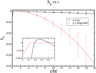
Figure 3: Plot of the $00$ component of the metric perturbation along the $x$-axis (solid line) and along the $y$-$z$ diagonal (dashed line) with the plotting parameters described in Sec. II.

Observe that the perturbation diverges as $r\to\infty$ and as $r\to 0$ along the $x$-axis, but it remains finite as $r\to 0$ along the $y$-$z$ diagonal. Everywhere else, and in particular near the outer horizon, the perturbation is of $O(V^{2})$, where $V=(M/b)^{1/2}$ is the orbital velocity. Finally, observe that the perturbation vanishes close but not really at either horizon, remaining finite through them.

The divergence of the perturbation can be used to approximately determine the region of validity of the approximation. As we have discussed previously and seen in Fig. 3, the perturbation will be valid inside a shell centered at the background hole. The inner radius of this shell can be approximately determined by graphically studying the radius where $h_{ab}>O(V^{2})$, approximately given by $r_{inner}\approx 0.01M$. This value for the inner radius of the shell is only an order of magnitude estimate, but is suffices to see that $r_{inner}\ll r_{-}$. The causal structure of the region $r<r_{-}$ is extremely complex and many of its features are known to be unstable under small perturbations that destroy the symmetries of the spacetime Poisson (2004b). However, note that the perturbation is well behaved for $r-r_{-}\ll M$ and in particular it is of the order predicted by the approximation [$O(V^{2})$]. In any case, the region $r<r_{-}$ is hidden inside the event horizon and most astrophysical applications will be concerned with regions of small spacelike separations from the outer horizon, and not the inner one.

The outer radius of the shell can be estimated by studying the fractional error in the perturbation, which is determined by comparing the perturbation to the uncontrolled remainders in the approximation. The approximate error bars in Fig. 3 are given by an estimate of these uncontrolled remainders, $\delta h_{ab}$, which are due to truncating the formal series solution at a finite order. In the present case, this truncation is done at $O(V^{2})$, where the tidal fields provide this scaling. The uncontrolled remainders then will be of $O(V^{3})$ and should come from time derivatives of the tidal tensors, i.e. $\delta h_{ab}\propto\dot{h}_{ab}$. The argument of the tidal tensors is $\omega v$, where $\omega=V/b$ is the angular velocity and where $v$ is the advanced time coordinate. Any time derivative will pull out a factor of $\omega$, which will in turn increase the order of that term. However, in order for the uncontrolled remainders to be dimensionally consistent ($\delta h_{ab}$ must have the same dimensions as $h_{ab}$), we need to multiply the time derivatives of the tidal tensors by $r$, so that

$$\delta h_{ab}\approx r\dot{h}_{ab}\approx r(V/b)h_{ab}.$$ (60)

This line of reasoning, however, only leads to an order of magnitude estimate of the uncontrolled remainder. In principle, any dimensionless scalar function could be multiplying this estimate as long as it does not change the scaling. For the case of non-spinning holes, the metric perturbation has been computed to $O(V^{3})$ Poisson (2005), which allows us to compare these terms to Eq. (60). This comparison suggests that the multiplicative scalar function is roughly unity and, thus, unnecessary so that Eq. (60) is indeed a good approximation to the scaling of the uncontrolled remainders. Clearly, this estimate is not the exact error in the approximation, which can formally only be determined if we know the exact functional form of the next order term. This estimate, however, is a physically well-motivated approximation for the uncontrolled remainders.

The outer radius of the region of validity of this approximation can be approximately determined by studying the behavior of these error bars. From Fig. 3 we see that the error bars become considerable large (approximately $50\%$ as big as the perturbation itself) roughly at $r=13M$. However, for $r<4M$ the estimated error bars are less than $10\%$ relative to the perturbation. This seems to indicate that, even at $b=10M$ where the slow-motion approximation begins to become inaccurate, the approximate solution is still valid sufficiently close to the outer horizon. This estimation of the fractional errors is by no means a formal proof of the existence or size of the region of validity of the approximation. However, this estimation does provide a strong argument that the approximation is indeed valid sufficiently close to the outer horizon. If $10\%$ fractional error is tolerable, which would correspond to neglecting terms of $O(V^{3})$, then the outer radius of the shell is approximately given by $r_{outer}\approx 4M$. Clearly, as $b$ is increased, the slow-motion approximation will become more accurate and, thus, the perturbation will be valid inside a bigger shell with larger outer radii.

The results of this paper are clearly valid close to the outer horizon of the background hole, thus allowing the study of physical processes of interest to the relativity community. For instance, we can use the perturbation presented here to construct initial data for a binary system near either hole. In this case, we are not interested in the behavior of the perturbation inside the inner horizon because that region can be excised and does not belong to the computational domain. Furthermore, the calculations of angular momentum and mass flux across the horizon can still be performed because they only depend on the behavior of the perturbation near or at the outer horizon.

V Conclusions

We have computed a tidally perturbed metric for a spinning black hole in the slow-motion approximation. This approximation allows us to parameterize the NP scalar $\psi_{0}$ [Eq. (17)] in terms of the electric and magnetic tidal tensors of the external universe. With this scalar we can then construct a potential $\Psi$ [Eq. (34)], by applying certain differential operators to it. From this potential, we can then apply the Chrzanowski procedure to construct a metric perturbation [Eqs. (III),(IV),(IV.1),(IV.2),(IV.2),(IV.2),(59)].

The metric is naturally computed in the ingoing radiation gauge and in Kerr coordinates, which are suitable to study perturbation near the horizon due to its horizon penetrating properties. This metric is given explicitly in terms of scalar functions of the coordinates and is parametrized by the mass of the background hole, its Kerr spin parameter and electric and magnetic tidal tensors. The mass and the spin parameters of the background hole do not have to be small relative to each other, so in principle the metric presented here is capable of representing tidally perturbed extremal Kerr holes. The tidal tensors describe the time-evolution of the perturbation produced by the external universe and, thus, are functions of time that should be determined by matching the metric to another approximation valid far from the holes.

The slow motion approximation constrains what kind of perturbations are allowed, thus limiting the external universe that is producing them. In this approximation, the radius of curvature of the external universe must be changing sufficiently slowly relative to the scales of the background hole. One consequence of this restriction is that the tidal fields must be slowly-varying functions of time, thus allowing us to neglect their time derivatives. In this sense, this approximation leads to a quasi-static limit, where in this paper we have calculated the first non-vanishing deviations from staticity. Another consequence of this approximation is that we can parametrized the perturbation in terms of multipole moments, where here we have only considered the first non-vanishing one (the quadrupolar perturbation). In perturbation theory, the $l+1$ mode will be one order smaller than the $l$ mode, which allows us to neglect the octopole and any other higher modes, as well as any mode beating between the quadrupole and higher modes.

Due to these restrictions, if we allow the external universe to be given by another hole in a quasicircular orbit around the background (a binary system), we are limited to those whose separation is sufficiently large. In this case, we must have sufficiently large orbital separations so that the Riemann curvature produced by the companion is large relative to the scales of the background hole. In other words, this approximation will break if we consider systems that are close to their innermost stable orbit and ready to plunge. We have seen, however, that for a separation of $b=10M$, the metric presented here is valid inside a shell given approximately by $0.01M<r<4M$.

The reason why the region of validity of the approximation is a shell can be traced back to the choice of tetrad and to the limitations of the Chrzanowski procedure. The perturbation cannot be valid too close to the background hole because in that region the Kinnersly tetrad, from which the perturbation was constructed, is also divergent. This perturbation is also divergent as $r\to\infty$ because the Chrzanowski procedure builds the perturbation as a linear expansion of the metric. In other words, we cannot analyze the dynamics of the entire spacetime with this metric, since its validity is limited to field points sufficiently close to the outer horizon of the background hole. However, if this metric were to be asymptotically matched to another metric valid far from the background hole, then the resultant metric would be accurate on the entire $3$-manifold up to uncontrolled remainders thus, capable of reproducing the dynamics of the entire spacetime.

This metric might be useful to different areas in general relativity. On the one hand it might be useful in the construction of astrophysically realistic initial data for binary systems of spinning black holes. Its importance relies in that it could accurately represent the metric field in the neighborhood of a black hole tidally disrupted by a companion. These tides are analytic and arise as a true approximate solution to the Einstein equations in the slow-motion approximation. Initial data, however, requires a metric that is valid in the entire $3$-manifold. Therefore, in order to use these results as initial data they will first have to be asymptotically matched Alvi (2000); Yunes et al. (2005) to a PN expansion valid far from the background holes Blanchet (2002). In this manner, initial data could be constructed that satisfies the full set of the Einstein equation, including the constraints, to a high order of accuracy.

Another use for the metric computed in this paper relates to the flux of mass and angular momentum through a perturbed Kerr horizon. This flux will be important for EMRIs, where the effect of tidal perturbations could be large enough to lead to large fluxes, which in turn could affect the gravitational wave signal emitted by the system Martel (2004); Hughes (2001). Recent investigations Poisson (2004a) have used a curvature formalism to compute this flux directly from $\psi_{0}$. However, there exists a metric formalism to obtain this flux directly from the metric itself. An interesting research direction would be to compute this flux and compare to the results obtained with the curvature formalism.

Finally, the perturbed metric computed here can also be of use to the data analysis community to construct gravitational waveforms. EMRIs are particularly good candidates to be observed by LISA, but such observations require extremely accurate formulae for the phasing of the gravitational waves due to the use of matched filtering. Recently, Ref. Glampedakis and Babak (2005) studied how to use and implement a quasi-Kerr metric (a perturbed Kerr metric in the limit of slow rotation of the background hole) to detect EMRIs with LISA. A similar study could be performed with the perturbed metric computed in this paper, which can also describe rapidly rotating black holes.

Future work will concentrate on performing the necessary asymptotic matching to shape this metric into useful initial data for numerical relativity applications. The matching procedure will provide expressions for the tidal tensors in terms of PN quantities, as well as a coordinate transformation between Kerr coordinates and the coordinate system used in the PN approximation. In this manner, a piece-wise global solution can be computed, which will contain small discontinuities inside the matching region that could be eliminated by the introduction of transition function. Since these discontinuities will be small due to the matching, the transition functions will not alter the content of the data to the order of the approximation used. After the matching is completed, we will have obtained an approximate analytic global metric that will contain the tidal fields of one hole on the other near the outer horizon of the former, where these fields come directly from solutions to the Einstein equations.

Appendix

In this appendix we provide explicit formula for the transformation from Kerr coordinates to Kerr-Schild coordinate. This transformation can be found in Refs. Misner et al. (1970); Carrol (2003); D’Inverno (1992) and is given by

$$x = \sin{\theta}\left(r\cos{\phi}-a\sin{\phi}\right),$$

$$y = \sin{\theta}\left(r\sin{\phi}+a\cos{\phi}\right).$$

$$z = r\cos{\theta}.$$ (61)

The inverse transformation is given by

$$r = \sqrt{\frac{R^{2}-a^{2}+w}{2}},$$

$$w = \sqrt{(R^{2}-a^{2})^{2}+4a^{2}z^{2}},$$

$$\theta = \arccos{\frac{z}{r}},$$

$$\phi = \arctan{\frac{ry-ax}{rx+ay}}.$$ (62)

Other useful relations are

$$\sin{\theta} = \left(\frac{x^{2}+y^{2}}{r^{2}+a^{2}}\right)^{1/2},$$

$$\sin{\phi} = \frac{ry-ax}{\left[(r^{2}+a^{2})(x^{2}+y^{2})\right]^{1/2}},$$

$$\cos{\phi} = \frac{rx+ay}{\left[(r^{2}+a^{2})(x^{2}+y^{2})\right]^{1/2}}.$$ (63)

Note that these transformation reduce to the usual transformation from spherical polar coordinates to Cartesian coordinates in the limit $a\to 0$.

The Jacobian of the transformation, $\Lambda^{a}{}_{b}=\partial x^{a}/\partial x^{b}$, is given explicitly by

$$\Lambda^{r}{}_{x} = \frac{x}{2r}\left(1+\frac{R^{2}-a^{2}}{w}\right),$$

$$\Lambda^{r}{}_{y} = \frac{y}{2r}\left(1+\frac{R^{2}-a^{2}}{w}\right),$$

$$\Lambda^{r}{}_{z} = \frac{z}{2r}\left(1+\frac{R^{2}+a^{2}}{w}\right),$$

$$\Lambda^{\theta}{}_{x} = \frac{zx}{2r^{2}}\left(1+\frac{R^{2}-a^{2}}{w}\right)\left(r^{2}-z^{2}\right)^{-1/2},$$

$$\Lambda^{\theta}{}_{y} = \frac{zy}{2r^{2}}\left(1+\frac{R^{2}-a^{2}}{w}\right)\left(r^{2}-z^{2}\right)^{-1/2},$$

$$\Lambda^{\theta}{}_{z} = -\left(r^{2}-z^{2}\right)^{-1/2}\left[1-\frac{z^{2}}{2r^{2}}\left(1+\frac{R^{2}+a^{2}}{w}\right)\right],$$

$$\Lambda^{\phi}{}_{x} = \frac{rx+ay}{(r^{2}+a^{2})(x^{2}+y^{2})}\left[\left(y-x\frac{ry-ax}{rx+ay}\right)\left(1\right.\right.$$

$$\left.\left.+\frac{R^{2}-a^{2}}{w}\right)\frac{x}{2r}-a-r\frac{ry-ax}{rx+ay}\right],$$

$$\Lambda^{\phi}{}_{y} = \frac{rx+ay}{(r^{2}+a^{2})(x^{2}+y^{2})}\left[\left(y-x\frac{ry-ax}{rx+ay}\right)\left(1\right.\right.$$

$$\left.\left.+\frac{R^{2}-a^{2}}{w}\right)\frac{y}{2r}+r-a\frac{ry-ax}{rx+ay}\right],$$

$$\Lambda^{\phi}{}_{z} = \frac{rx+ay}{(r^{2}+a^{2})(x^{2}+y^{2})}\left[\left(y-x\frac{ry-ax}{rx+ay}\right)\left(1\right.\right.$$

$$\left.\left.+\frac{R^{2}+a^{2}}{w}\right)\frac{z}{2r}\right].$$

Note that this Jacobian reduces to the standard Jacobian of the transformation between spherical polar and Cartesian coordinates in the limit $a\to 0$. There is a more elegant way to write this Jacobian in tensor notation as

$$\Lambda^{r}{}_{a} = \frac{1}{2r}\left\{\delta_{ai}x^{i}+\frac{1}{w}\left[\delta_{ia}x^{i}\left(R^{2}-a^{2}\right)+2a^{2}z\delta_{az}\right]\right\},$$

$$\Lambda^{\theta}{}_{a} = \frac{z}{r\left(r^{2}-a^{2}\right)^{1/2}}\Lambda^{r}{}_{a},$$

$$\Lambda^{\phi}{}_{a} = \frac{rx+ay}{(r^{2}+a^{2})(x^{2}+y^{2})}\left[\Lambda^{r}{}_{a}\left(y-\frac{ry-ax}{rx+ay}x\right)\right.$$

$$\left.+\left(r-\frac{ry-ax}{rx+ay}a\right)\delta_{ya}-\left(a+\frac{ry-ax}{rx+ay}r\right)\delta_{xa}\right].$$

With this Jacobian, the metric in Kerr-Schild coordinates is given by

$$g_{ab}=g_{a^{\prime}b^{\prime}}\Lambda^{a^{\prime}}{}_{a}\Lambda^{b^{\prime}}{}_{b},$$ (66)

where here the primed indices refer to spherical coordinates and the unprimed indices to Cartesian coordinates.

References

- Cutler and Thorne (2002) C. Cutler and K. S. Thorne (2002), eprint gr-qc/0204090.
- Poisson (2004a) E. Poisson, Phys. Rev. D70, 084044 (2004a), eprint gr-qc/0407050.
- Poisson and Sasaki (1995) E. Poisson and M. Sasaki, Phys. Rev. D51, 5753 (1995), eprint gr-qc/9412027.
- Tagoshi et al. (1997) H. Tagoshi, S. Mano, and E. Takasugi (1997), prepared for APCTP Workshop: Pacific Particle Physics Phenomenology (P4 97), Seoul, Korea, 31 Oct - 2 Nov 1997.
- Alvi (2001) K. Alvi, Phys. Rev. D64, 104020 (2001), eprint gr-qc/0107080.
- Martel (2004) K. Martel, Phys. Rev. D69, 044025 (2004), eprint gr-qc/0311017.
- Hughes (2001) S. A. Hughes, Phys. Rev. D64, 064004 (2001), eprint gr-qc/0104041.
- Glampedakis and Babak (2005) K. Glampedakis and S. Babak (2005), eprint gr-qc/0510057.
- Alvi (2000) K. Alvi, Phys. Rev. D61, 124013 (2000), eprint gr-qc/9912113.
- Yunes et al. (2005) N. Yunes, W. Tichy, B. J. Owen, and B. Bruegmann (2005), eprint gr-qc/0503011.
- D’Eath (1975a) P. D. D’Eath, Phys. Rev. D11, 1387 (1975a).
- D’Eath (1975b) P. D. D’Eath, Phys. Rev. D12, 2183 (1975b).
- D’Eath (1996) P. D. D’Eath, Bkack holes: Gravitational interactions (Clarendon Press, Oxford, 1996).
- Poisson (2005) E. Poisson, Phys. Rev. Lett. 94, 161103 (2005), eprint gr-qc/0501032.
- Regge and Wheeler (1957) T. Regge and J. Wheeler, Phys. Rev. 108, 1063 (1957).
- Chrzanowski (1975) P. L. Chrzanowski, Phys. Rev. D 11, 2042 (1975).
- Ori (2003) A. Ori, Phys. Rev. D67, 124010 (2003), eprint gr-qc/0207045.
- Burke and Thorne (1970) W. L. Burke and K. S. Thorne, in Relativity, edited by M. Carmeli, S. I. Fickler, and L. Witten (Plenum Press, 1970), pp. 209–228.
- Burke (1971) W. L. Burke, J. Math. Phys. 12, 401 (1971).
- Thorne and Hartle (1985) K. S. Thorne and J. B. Hartle, Phys. Rev. D31, 1815 (1985).
- Baumgarte (2000) T. W. Baumgarte, Phys. Rev. D 62, 024018 (2000), eprint gr-qc/0004050.
- Grandclement et al. (2002) P. Grandclement, E. Gourgoulhon, and S. Bonazzola, Phys. Rev. D65, 044021 (2002), eprint gr-qc/0106016.
- Wald (1978) R. M. Wald, Phys. Rev. Lett. 41, 203 (1978).
- Kegeles and Cohen (1979) L. S. Kegeles and J. M. Cohen, Phys. Rev. D19, 1641 (1979).
- Campanelli and Lousto (1999) M. Campanelli and C. O. Lousto, Phys. Rev. D59, 124022 (1999), eprint gr-qc/9811019.
- Bender and Orszag (1999) C. M. Bender and S. A. Orszag, Advanced mathematical methods for scientists and engineers 1, Asymptotic methods and perturbation theory (Springer, New York, 1999).
- Blanchet (2002) L. Blanchet, Living Rev. Relativity 5, 3. URL (cited on 5 January 2006) (2002), and references therein, eprint http://www.livingreviews.org/lrr-2002-3.
- Ansorg and Petroff (2005) M. Ansorg and D. Petroff, Phys. Rev. D72, 024019 (2005), eprint gr-qc/0505060.
- Poisson (2004b) E. Poisson, A relativist’s toolkit (Cambrdige, 2004b).
- Press and Teukolsky (1973) W. H. Press and S. A. Teukolsky, Astrophys. J. 185, 649 (1973).
- Lousto and Whiting (2002) C. O. Lousto and B. F. Whiting, Phys. Rev. D66, 024026 (2002), eprint gr-qc/0203061.
- Chandrasekhar (2000) S. Chandrasekhar, The Mathematical Theory of Black Holes (Clarendon Press, Oxford, 2000).
- Misner et al. (1970) C. Misner, K. Thorne, and J. Wheeler, Gravitation (Freeman, 1970).
- Carrol (2003) S. M. Carrol, An introduction to general relativity, Spacetime and Geometry (Pearson - Benjamin Cummings, San Francisco, 2003).
- D’Inverno (1992) R. D’Inverno, Introducing Einstein’s Relativity (Oxford University press, Oxford, 1992).