Maxwell-type behavior from a geometrical structure

Abstract

We study which geometric structure can be constructed from the vierbein (frame/coframe) variables and which field models can be related to this geometry. The coframe field models, alternative to GR, are known as viable models for gravity, since they have the Schwarzschild solution. Since the local Lorentz invariance is violated, a physical interpretation of additional six degrees of freedom is required. The geometry of such models is usually given by two different connections — the Levi-Civita symmetric and metric-compatible connection and the Weitzenböck flat connection.

We construct a general family of linear connections of the same type, which includes two connections above as special limiting cases. We show that for dynamical propagation of six additional degrees of freedom it is necessary for the gauge field of infinitesimal transformations (antisymmetric tensor) to satisfy the system of two first order differential equations. This system is similar to the vacuum Maxwell system and even coincides with it on a flat manifold. The corresponding “Maxwell-compatible connections” are derived. Alternatively, we derive the same Maxwell-type system as a symmetry conditions of the viable models Lagrangian. Consequently we derive a nontrivial decomposition of the coframe field to the pure metric field plus a dynamical field of infinitesimal Lorentz rotations. Exact spherical symmetric solution for our dynamical field is derived. It is bounded near the Schwarzschild radius. Further off, the solution is close to the Coulomb field.

1 Introduction

GR is a classical field theory for 10 independent variables — the components of metric tensor $g_{ij}$. It is well known, however, that some problems inside and beyond Einstein’s gravity require a richer set of 16 independent variables — the components of the coframe (aka reper, vierbein, …). In the following issues of gravity, the coframe is not only a useful tool but often cannot even be replaced by the standard metric variable:

• Hamiltonian formulation [1],[2] ;

• Positive energy proofs [3];

• Fermions on a curved manifold [4],[5];

• Supergravity [6];

• Loop quantum gravity [7], [8].

Absolute (teleparallel) frame/coframe variables were introduced in physics by Einstein in 1928 with an aim of a unification of gravitational and electromagnetic fields (for classical references, see [9]). In GR description, the additional six degrees of freedom do not have a physical sense and treated as a type of a gauge symmetry of the metric tensor.

It was already noticed by Einstein, that 16 reper components cannot be completely equivalent to 10 components of the metric tensor. Indeed, the supergravity and the loop quantum gravity models apparently can be formulated only in term of vierbein. So, it is natural to study which geometric structure can be constructed from the vierbein (frame/coframe) variables and which field models can be related to this geometry. This is a subject of the current paper.

The frame field $e_{\alpha}$ and its dual, the coframe field $\vartheta^{\alpha}$, have a well defined geometrical sense. In particular, even been considered as independent physical fields, they provide a special (absolute) reference basis. For the bases, $\{e_{\alpha}\,,\vartheta^{\alpha}\}$, fixed at a point, the construction gives an invariant meaning to the components of a tensor, thus it emerges in violation of the rotational and Lorentz invariance [10]. However, when the global (rigid) Lorentz transformations of the absolute basis fields are acceptable, the frame components of a tensor are transformed merely by the Lorentz transformation law. Thus, some interrelation between the Lorentz invariant field theories and the diffeomorphism invariant gravity emerges. When the absolute basis field is restricted to a point, the Lorentz invariance requires to consider it not alone but as a member of a class of equivalent bases. The equivalence relation for this class is provided by a group $G$ of transformations $\vartheta^{\alpha}\to L^{\alpha}{}_{\beta}\,\vartheta^{\beta}$, which has to include local physics symmetries, i.e., the rotations and the boosts.

When we are dealing with the absolute basis fields on a manifold, the relation between the frames at different points is not governed by the constrains of local physics. Consequently, three principally different possibilities are open:

(i) Riemannian geometry. The frames at distinct points are not related to one another at all, i.e. the dependence of the elements of the group $G$ on a point is absolutely arbitrary. It is possible only if the corresponding geometry, i.e the metric and the connection, respect the arbitrary transformations of the frame field. The unique connections with this property is the Levi-Civita connection of Riemannian geometry. This case is realized in the standard GR when it is formulated in an arbitrary non-holonomic frame. The frame/coframe fields are not physical in this case and only play a role of a useful reference tool. They can be replaced even by holonomic bases generated by local coordinates.

(ii) Teleparallel geometry. Another limiting case emerges when the frames in distinct points are strongly connected to one another. It means that when a frame in an arbitrary point is rotated in a certain angle, the frames at distant points immediately rotated in the same angle. The unique connection with this property is the flat Weitzenböck connection. Although the scalar curvature is zero for such a connection, the action functional can be constructed from the torsion tensor. It is natural to require this action functional to be invariant only under global transformations of the basis field. The analysis of this model shows that it has not spherical symmetric solutions with Newtonian behavior at infinity. As a result, this absolute teleparallel gravity model is not physical.

(iii) Gauge geometry. Besides the two limiting cases given above, there is a family of geometries with the field of frame rotations satisfying some system of differential equations. The basic geometrical quantities, metric and connection, have to be invariant under local transformations of the frame field satisfied these equations. In this construction, the frame field does not emerge explicitly, so we will refer to the corresponding geometrical structure as a gauge coframe geometry.

In alternative gravity models (see [11] — [20] and the reference given therein), the frame variable appears as an independent physical field. In the first order approximation [21], the coframe field is separated to a sum of two independent fields - a metric field and an antisymmetric field of the rang two. The same separation emerges in the Lagrangian, in the field equation and also in the energy-momentum tensor. In the current paper we show that a geometrical and physical interpretation of the antisymmetric part can be prolongated in the higher order approximations. Our main result is: In the viable coframe models, alternative to GR, the additional degrees of freedom can be interpreted as a new dynamical field which behavior in the first order approximation is described by the vacuum Maxwell-type system.

1.1 Overview

The aim of this paper is to derive the mentioned coframe gauge geometrical structure and its possible applications to classical fields. The paper is organized as followed.

In section 2, we construct a most general class of connections which are linear in the first order derivatives of the coframe field. This six-parametric family involves the Levi-Civita and the Weitzenböck connections as special limiting cases. We also identify the sub-families of torsion-free and metric compatible connections.

In section 3, the behavior of the coframe connections under local $SO(1,3)$ transformations of the coframe is considered. Besides the Levi-Civita and the Weitzenböck connections, we identify a sub-family of gauge invariant connections. The corresponding constraints compose a system of 8 first order partial differential equation for six independent entries of a $SO(1,3)$ matrix. This situation is very similar to the standard Maxwell system of eight field equations for six independent components of the electromagnetic field.

In section 4, we derive the same system of constrains from a different (physical) point of view. We require a most general quadratic coframe Lagrangian to be invariant under $SO(1,3)$ transformations of the coframe. The gauge invariant Lagrangians turn out to be in a correspondence with the known viable coframe models having the Schwarzschild solution.

In section 5, we study the first order approximation to the system of the constrains. On a flat manifold, this system coincides with the vacuum Maxwell equations. On a curved manifold, it turns out to be a system of covariant Maxwell-type equations when the covariant derivatives are considered relative to the Weitzenböck connections.

In section 6, we derive an exact spherical symmetric solution to our system of constrains. We also compare our model with the standard description of interaction between gravitational and electromagnetic fields. In contrast to the standard Einstein-Maxwell system, our model predicts mass dependence in the Coulomb-type law. We derive the exact expression of the corresponding correction term.

In section 7, we give an outlook of the proposed alternative model and discuss how (and if) the additional degrees of freedom can be related to the ordinary electromagnetic field.

1.2 Notations

We use the Greek indices $\alpha\,,\beta\,,\cdots=0,1,2,3$ to identify the specific vector fields of the frame $e_{\alpha}$ and the specific 1-forms of the coframe $\vartheta^{\alpha}$. The Roman indices $i\,,j\,,\cdots=0,1,2,3$ refer to local coordinates. Summation from 0 to 3 is understood over repeated indices of both types (Einstein’s summation convention). Two types of indices and basically different. In particular, they cannot be summed (contracted) in the expressions ${\vartheta^{\alpha}}_{a}$ or ${e_{\alpha}}^{a}$. The Lorentz metric is used with the sign agreement $\eta_{\alpha\beta}={\rm diag}(-1,1,1,1)$. The spatial indices are denoted as ${\hat{i}}\,,{\hat{j}}\,,\cdots=1,2,3$.

We denote the coefficients of connection as $\Gamma_{ij}{}^{k}$ and $\Gamma_{ijk}=g_{km}\Gamma_{ij}{}^{m}$. Such notation is useful for the exterior form representation [22]. In order to go back to the ordinary tensorial notations $\Gamma^{k}_{ij}$, it is enough to move the last index to the first position.

The symmetrization and antisymmetrization operators are used in the normalized form, i.e., $A_{(i_{1}\cdots i_{p})}=(1/{p!})(A_{i_{1}\cdots i_{p}}+\cdots)$ and $A_{[i_{1}\cdots i_{p}]}=(1/{p!})(A_{i_{1}\cdots i_{p}}-\cdots)$.

2 Coframe connections

2.1 Coframe structure

Let a $4D$-manifold be endowed with a frame field $e_{\alpha}$ and a coframe field $\vartheta^{\alpha}$. All the structures are assumed to be smooth almost everywhere. In local coordinates $x^{i}$, the fields are expressed respectively as

$$e_{\alpha}={e_{\alpha}}^{i}\,\partial_{i}\,,\qquad\vartheta^{\alpha}={\vartheta^{\alpha}}_{i}\,dx^{i}\,,$$ (2.1)

i.e., by two $4\times 4$ matrices ${e_{\alpha}}^{i}(x)$ and ${\vartheta^{\alpha}}_{i}(x)$ of smooth functions. These two basis fields are assumed to be reciprocal to each other:

$${e_{\alpha}}^{i}\,{\vartheta^{\beta}}_{i}=\delta^{\beta}_{\alpha}\,,\qquad{e_{\alpha}}^{i}\,{\vartheta^{\alpha}}_{j}=\delta^{i}_{j}\,.$$ (2.2)

So, in fact, only one field, $e_{\alpha}$ or $\vartheta^{\alpha}$, is an independent variable. We prefer to use the coframe field $\vartheta^{\alpha}$ as a basis variable since it is suitable for a compact exterior form representation.

For a rigidly fixed coframe field, the components of an arbitrary tensor obtain an invariant sense when referred to the special bases $e_{\alpha}\,,\vartheta^{\alpha}$. It emerges in hard violation of Lorentz invariance. Thus, in order to have a Lorentz invariant field model, the coframe field has to be defined only up to global Lorentz transformations. The gauge paradigm requires to localize the global transformations, so we define a coframe structure as a triplet

$$\{{\mathcal{M}}\,,\,\vartheta^{\alpha}\,,\,G\}\,,$$ (2.3)

where ${\mathcal{M}}$ is a smooth manifold, $\vartheta^{\alpha}$ is a smooth coframe field on ${\mathcal{M}}$, and $G=\{L^{\alpha}{}_{\beta}(x)\}$ is a local (pointwise) group of transformations $\vartheta^{\alpha}\to L^{\alpha}{}_{\beta}(x)\vartheta^{\beta}$. Although the coframe variable itself is a pure geometrical object, it is not clear what geometry is generated by the structure (2.3) for different groups $G$.

We accept the Cartan viewpoint that treats a geometrical structure as a pair of two independent objects: a metric tensor $g_{ij}(x)$ and an asymmetric connection field $\Gamma_{ij}{}^{k}(x)$. For the specific coframe structure (2.3), we require both fields to be explicitly constructed from the coframe components. In other words, we specify (2.3) to

$$\{{\mathcal{M}}\,,\,g_{ij}(\vartheta^{\alpha})\,,\,\Gamma_{ij}{}^{k}(\vartheta^{\alpha})\,,\,G\}\,.$$ (2.4)

In correspondence to local physics, the metric tensor has to be defined as

$$g=\eta_{\alpha\beta}\,\vartheta^{\alpha}\otimes\vartheta^{\beta}\,,$$ (2.5)

or, in components,

$$g_{ij}=\eta_{\alpha\beta}\,\vartheta^{\alpha}{}_{i}\,\vartheta^{\beta}{}_{j}\,,\qquad g^{ij}=\eta^{\alpha\beta}\,e_{\alpha}{}^{i}\,e_{\beta}{}^{j}\,.$$ (2.6)

Here $\eta_{\alpha\beta}$ is the Lorentzian metric in the tangential vector space. Indeed, in a small neighborhood of a point, the coframe field is approximately holonomic $\vartheta^{\alpha}{}_{i}=\delta^{\alpha}_{i}$, so (2.6) is locally approximated by Lorentzian metric, see [21]. Due to the index content, (2.5) is a unique construction up to a constant scalar factor. This factor can be neglected by rescaling the coframe field (recall that the global $GL(4,\mathbb{R})$-transformations of the structure are admissible). Hence (2.5) is a unique construction of the metric tensor from the coframe components when the conformation with the local Lorentz metric is required. This definition restricts the freedom of the coframe transformation to local pseudo-rotations, i.e., at every point $G=SO(1,3)$. The entries of this $SO(1,3)$-matrix remain arbitrary functions of a point.

2.2 Coframe connections

Let a manifold be endowed with a field of asymmetric Cartan connections. Relative to a local coordinate chart $x^{i}$, every connection is represented by a set of $4^{3}$ independent functions ${\Gamma_{ij}}^{k}(x)$ — the coefficients of the connection. The only condition the functions ${\Gamma_{ij}}^{k}(x)$ have to satisfy is to transform, under a change of coordinates $x^{i}\mapsto y^{i}(x^{j})$, by an inhomogeneous linear rule:

$$\Gamma_{ij}{}^{k}\mapsto\Big{(}\Gamma_{lm}{}^{n}y^{l}{}_{,i}y^{m}{}_{,j}+y^{n}{}_{,ij}\Big{)}x^{k}{}_{,n}\,,$$ (2.7)

where the derivatives are denoted as $y^{i}{}_{,j}={\partial y^{i}}/{\partial x^{j}}$ and $x^{i}{}_{,j}={\partial x^{i}}/{\partial y^{j}}$.

For the coframe connections, we require $\Gamma_{ij}{}^{k}$ and $\Gamma_{ijk}=g_{km}\Gamma_{ij}{}^{m}$ to be explicitly constructed from the coframe components and their derivatives. Moreover, we require $\Gamma_{ij}{}^{k}$ to be linear in $\vartheta^{\alpha}{}_{m,n}$ — linear connection. This requirement is in parallel to the standard construction of Riemannian geometry. Indeed, the Levi-Civita connection can be treated as a unique linear connection which can be constructed from the first order derivatives of the metric components $g_{ij,k}$.

Two examples of the coframe connection satisfied the requirement above are well known:

(i) The Weitzenböck connection is defined as

$$\stackrel{{\scriptstyle{\rm o}}}{{\Gamma}}{\!}_{ij}{}^{k}={e_{\alpha}}^{k}\,{\vartheta^{\alpha}}_{i,j}\,,\qquad\stackrel{{\scriptstyle{\rm o}}}{{\Gamma}}{\!}_{ijk}=\eta_{\alpha\beta}\vartheta^{\alpha}{}_{k}\vartheta^{\beta}{}_{i,j}\,.$$ (2.8)

It is straightforward to check the transformation rule (2.7) for this expression. The Riemann curvature of this connection is identically zero, so the connection is flat. We denote the antisymmetric combination (torsion) of (2.8) and its trace as

$$C_{ijk}=\stackrel{{\scriptstyle{\rm o}}}{{\Gamma}}{\!}_{[ij]k}\,,\qquad C_{i}=C_{mi}{}^{m}\,.$$ (2.9)

When the transformation (2.7) is applied to these quantities, the inhomogeneous parts are canceled. Consequently, (2.9) change as tensors under the transformations of coordinates. Their behavior under local transformations of the coframe is an independent property, which we will examine in the consequence.

(ii) The Levi-Civita connection of Riemannian geometry,

$$\stackrel{{\scriptstyle{\rm*}}}{{\Gamma}}{\!}_{ij}{}^{k}=\frac{1}{2}g^{km}(g_{im,j}+g_{jm,i}-g_{ij,m})\,,$$ (2.10)

can be rewritten as a linear combination of the first order derivatives of the coframe components. Indeed, we substitute (2.5) into (2.10) to have

$$\stackrel{{\scriptstyle{\rm*}}}{{\Gamma}}{\!}_{ijk} = \eta_{\alpha\beta}\Big{(}\vartheta^{\alpha}{}_{k}\vartheta^{\beta}{}_{(i,j)}+\vartheta^{\alpha}{}_{j}\vartheta^{\beta}{}_{[k,i]}+\vartheta^{\alpha}{}_{i}\vartheta^{\beta}{}_{[k,j]}\Big{)}$$ (2.11)

$$= \stackrel{{\scriptstyle{\rm o}}}{{\Gamma}}{\!}_{(ij)k}+\stackrel{{\scriptstyle{\rm o}}}{{\Gamma}}{\!}_{[ki]j}+\stackrel{{\scriptstyle{\rm o}}}{{\Gamma}}{\!}_{[kj]i}$$

$$= \stackrel{{\scriptstyle{\rm o}}}{{\Gamma}}{\!}_{ijk}-C_{ijk}+C_{kij}+C_{kji}\,.$$

The transformation law (2.7) for this connection is a well known fact. The invariance of (2.11) under arbitrary local $SO(1,3)$-transformations of the coframe field is clear from (2.10).

We are looking now for a most general connection $\Gamma_{ijk}$ which is linear in the first order derivatives of the coframe, i.e., for a generalization of (2.8) and (2.11). Similarly to these special cases, the coefficients in the general linear combination of the first order derivatives have to be linear in the coframe components. In order to construct the most general coframe connection, we apply the well known fact: The difference of two arbitrary connections is a tensor. Thus a general coframe connection can be represented as the Weitzenböck connection plus a tensor,

$$\Gamma_{ijk}=\stackrel{{\scriptstyle{\rm o}}}{{\Gamma}}{\!}_{ijk}+Y_{ijk}\,,$$ (2.12)

or, alternatively, as the Levi-Civita connection plus a tensor,

$$\Gamma_{ijk}=\stackrel{{\scriptstyle{\rm*}}}{{\Gamma}}{\!}_{ijk}+Z_{ijk}\,.$$ (2.13)

The tensor $Y_{ijk}$ of (2.12) has to be itself linear in the first order derivatives of the coframe field. Consequently it can be written as

$$Y_{ijk}=\chi_{ijk}{}^{mnl}\Big{(}\eta_{\alpha\beta}\vartheta^{\alpha}{}_{l}\vartheta^{\beta}{}_{[m,n]}\Big{)}=\chi_{ijk}{}^{mnl}\,C_{mnl}\,.$$ (2.14)

The “constitutive tensor” $\chi_{ijk}{}^{mnl}$ can involve only the components of the metric tensor and the Kronecker symbols. In view of the symmetry relation $\chi_{ijk}{}^{mnl}=\chi_{ijk}{}^{[mn]l}$, it is enough to restrict the general expression to

$$\chi_{ijk}{}^{mnl} = \alpha_{1}\delta_{i}^{m}\delta_{j}^{n}\delta_{k}^{l}+g^{ml}(\alpha_{2}g_{ik}\delta_{j}^{n}+\alpha_{3}g_{jk}\delta_{i}^{n}+\beta_{1}g_{ij}\delta^{n}_{k})+$$ (2.15)

$$\quad\beta_{2}\delta^{m}_{k}\delta^{n}_{j}\delta^{l}_{i}+\beta_{3}\delta^{m}_{k}\delta^{n}_{i}\delta^{l}_{j}\,.$$

Substituting into (2.12) we have

$$\Gamma_{ijk} = \stackrel{{\scriptstyle{\rm o}}}{{\Gamma}}{\!}_{ijk}+\alpha_{1}C_{ijk}+\alpha_{2}g_{ik}C_{j}+\alpha_{3}g_{jk}C_{i}+$$ (2.16)

$$\qquad\quad\beta_{1}g_{ij}C_{k}+\beta_{2}C_{kji}+\beta_{3}C_{kij}\,,$$

or, equivalently,

$$\Gamma_{ij}{}^{k} = \stackrel{{\scriptstyle{\rm o}}}{{\Gamma}}{\!}_{ij}{}^{k}+\alpha_{1}C_{ij}{}^{k}+\alpha_{2}C_{j}\delta_{i}^{k}+\alpha_{3}C_{i}\delta^{k}_{j}+$$ (2.17)

$$g^{kn}\left(\beta_{1}g_{ij}C_{n}+\beta_{2}g_{im}C_{nj}{}^{m}+\beta_{3}g_{jm}C_{ni}{}^{m}\right)\,.$$

The $\alpha$-terms in (2.16) are defined already on a linear connection manifold without a metric, the $\beta$-terms require a metric structure on a manifold. We give an equivalent form of the family (2.17) via the Levi-Civita connection,

$$\Gamma_{ijk} = \stackrel{{\scriptstyle{\rm*}}}{{\Gamma}}{\!}_{ijk}+(\alpha_{1}+1)C_{ijk}+\alpha_{2}g_{ik}C_{j}+\alpha_{3}g_{jk}C_{i}+$$ (2.18)

$$\qquad\quad\beta_{1}g_{ij}C_{k}+(\beta_{2}-1)C_{kji}+(\beta_{3}-1)C_{kij}\,,$$

Hence, in contrast to Riemannian geometry with a unique Levi-Civita connection, we have, on the coframe manifold, an infinity 6-parametric family of connections constructed from the coframe components only.

2.3 Torsion of the coframe connections

On a linear connection manifold, an asymmetric connection is characterized by its torsion tensor which is defined as

$$T_{ij}{}^{k}=\Gamma_{[ij]}{}^{k}\,.$$ (2.19)

This skew-symmetric tensor ($T_{ij}{}^{k}=-T_{ji}{}^{k}$) does not depend on the metric structure. For the exterior form representation, see [22]—[26].

For the Weitzenböck connection, the torsion is given by $\stackrel{{\scriptstyle{\rm o}}}{{T}}{\!}_{ij}{}^{k}=C_{ij}{}^{k}$. Due to (2.8), this tensor is zero only for closed coframe 1-forms which satisfy $d\vartheta^{\alpha}=0$. The Levi-Civita connection is symmetric in the down indices, thus its torsion is zero.

The torsion tensor of the general connection (2.17) is given by

$$T_{ijk} = (\alpha_{1}+1)C_{ijk}+\frac{1}{2}(\alpha_{2}-\alpha_{3})(g_{ik}C_{j}-g_{jk}C_{i})+$$ (2.20)

$$\frac{1}{2}(\beta_{2}-\beta_{3})(C_{kji}-C_{kij})\,.$$

Consequently, the relations

$$\alpha_{1}=-1\,,\qquad\alpha_{2}=\alpha_{3}\,,\qquad\beta_{2}=\beta_{3}\,$$ (2.21)

extract a 3-parametric sub-family of identically symmetric (torsion-free) connections.

Geometrically, the non-zero torsion means a non-trivial parallel transport even on a flat manifold. The field models on a manifold with a connection of a non-zero torsion can include additional terms for interaction with torsion. The physical effects of a non-zero torsion was studied intensively, see the reports [30]—[32] and the references given therein. Probably the most important result of these numerous studies is the fact that non-zero torsion does not contradict the standard physical paradigm.

2.4 Non-metricity of the coframe connections

Another algebraic characteristic of an asymmetric connection can be given on a manifold endowed with a metric. The non-metricity tensor, $Q_{kij}=Q_{kji}$, is defined by the covariant derivative of the metric tensor,

$$Q_{kij}=-g_{ij;k}=-g_{ij,k}+\Gamma_{ikj}+\Gamma_{jki}\,.$$ (2.22)

where $\Gamma_{ijk}=\Gamma_{ij}{}^{m}g_{mk}$.

For the Weitzenböck and the Levi-Civita connections, the non-metricity tensor is zero. For the general connection (2.17), it is given by

$$Q_{kij} = (\alpha_{1}+\beta_{2})(C_{ikj}+C_{jki})+2\alpha_{2}g_{ij}C_{k}+$$ (2.23)

$$(\alpha_{3}+\beta_{1})(g_{ik}C_{j}+g_{jk}C_{i})\,.$$

Hence, the connection (2.12) is metric-compatible (has an identically zero tensor of non-metricity) if

$$\alpha_{1}=-\beta_{2}\,,\qquad\alpha_{2}=0\,,\qquad\alpha_{3}=-\beta_{1}\,.$$ (2.24)

Two tensors, the torsion an the non-metricity, characterize the affine connection uniquely [27]. In fact, we can decompose the general affine connection (2.17) as

$$\Gamma_{ijk} = \stackrel{{\scriptstyle{\rm*}}}{{\Gamma}}{\!}_{ijk}+(T_{ijk}+T_{kij}-T_{jki})+\frac{1}{2}(Q_{ijk}-Q_{kij}+Q_{jki})\,.$$ (2.25)

Consequently, a manifold endowed with an asymmetric connection can be treated as a Riemannian geometry with two additional tensors of torsion and non-metricity. Geometrically, a non-trivial non-metricity tensor means change of the lengths and angles when a parallel transport of vectors over a closed curve is applied. Such violation of rotational and Lorentz invariance bring us rather far from the standard physical paradigm. So, from the physical point of view, the metric-compatible constrains (2.24) are better motivated then the torsion-free constrains (2.21).

When the requirements (2.21,2.24) are considered together, we come to a unique torsion-free and metric-compatible coframe connection given by the parameters

$$\alpha_{1}=-1\,,\qquad\beta_{2}=\beta_{3}=1\,,\qquad\alpha_{2}=\alpha_{3}=\beta_{1}=0\,.$$ (2.26)

Certainly, it is no more than the ordinary Levi-Civita connection (2.10).

2.5 The Riemannian curvature of the coframe connections

Although the Riemannian curvature tensor is a classical subject of differential geometry, in the case of an asymmetric connection, slightly different notations are in use. We accept the agreements used in metric-affine gravity [22].

The Riemannian curvature tensor of a general asymmetric connection is defined as

$$R_{imn}{}^{j}=\Gamma_{im}{}^{j}{}_{,n}-\Gamma_{in}{}^{j}{}_{,m}+\Gamma_{in}{}^{k}\,\Gamma_{km}{}^{j}-\Gamma_{im}{}^{k}\,\Gamma_{kn}{}^{j}\,.$$ (2.27)

We are interested in the Riemannian curvature of the coframe connection (2.17). Due to (2.27), $R_{imn}{}^{j}$ involves the parameters $\alpha_{i},\beta_{i}$ in linear and quadratic combinations. It vanishes for zero values of the parameters, i.e., for the Weitzenböck connection. Moreover, the Weitzenböck connection $\stackrel{{\scriptstyle{\rm o}}}{{\Gamma}}{\!}_{ij}{}^{k}$ is a unique coframe connection of an identically zero curvature, for a proof, see [28].

For classical fields applications, we are interested in the scalar curvature, i.e., in the Hilbert-Einstein Lagrangian,

$${\mathcal{L}}=R\sqrt{-g}=g^{in}R_{ijn}{}^{j}\sqrt{-g}\,.$$ (2.28)

When (2.17) is substituted here, we obtain [28]

$$R\sqrt{-g}=C_{ijk}H^{ijk}\sqrt{-g}+{\rm\,\,total\,\,\,derivative}\,,$$ (2.29)

where

$$H^{ijk}=\rho_{1}\,C^{ijk}+3\rho_{2}C^{[ijk]}+\rho_{3}\Big{(}C^{ijk}-2\,C^{im}{}_{m}g^{jk}\Big{)}\,.$$ (2.30)

The dimensionless coefficients $\rho_{i}$ are quadratic polynomials in the constants $\alpha_{i},\beta_{i}$.

The quadratic part of the (2.29) is well known from the gravity fields models based on the coframe fields [11], [15], [24]. Up to a change of parameters, it is the most general scalar expression quadratic in the first order derivatives of the coframe field. Usually, this expression is treated as an arbitrary linear combination of the squares of the Weitzenböck torsion. Note certain outputs of our coframe connections approach:

• The quadratic coframe Lagrangian is regarded as a standard Einstein-Hilbert Lagrangian calculated on a general asymmetric coframe connection.

• The six-parametric connection (2.17) is involved in the Lagrangian (2.29) only via three independent combinations. Thus three additional requirements (for instance, the compatibility to the metric tensor) can be applied without changing the physical content of the model.

3 Gauge invariant connections

3.1 Gauge transformation

Let us examine now the behavior of the geometrical structure (2.4) under local transformations of the coframe field

$$\vartheta^{\alpha}\mapsto L^{\alpha}{}_{\beta}(x)\,\vartheta^{\beta}\,.$$ (3.1)

The metric tensor itself is invariant under local Lorentz transformations, thus, for every $x$, the matrix $L^{\alpha}{}_{\beta}(x)\in SO(1,3)$. Thus we are looking for a subclass of the connections (2.16) that invariant under pseudo-orthonormal transformations (3.1). Since the coframe field appears in (2.4) only implicitly, (3.1) is a type of gauge transformation. Certainly, the Levi-Civita connection is in the desired subclass. Consequently, our invariance condition does not bring us too far from the standard Riemannian geometry. Moreover, with this requirement, we can have only small additions also on the physical field level, see Sect 5.

In a coordinate basis, the coframe components change under (3.1) as

$$\vartheta^{\alpha}{}_{i}\mapsto L^{\alpha}{}_{\beta}\,\vartheta^{\beta}{}_{i}\,,\qquad e_{\alpha}{}^{i}\mapsto(L^{-1})^{\beta}{}_{\alpha}\,e_{\beta}{}^{i}\,.$$ (3.2)

In this paper, we will deal only with the infinitesimal version of the transformations (3.1). Consequently, we restrict to

$$L^{\alpha}{}_{\beta}=\delta^{\alpha}_{\beta}+X^{\alpha}{}_{\beta}\,.$$ (3.3)

Correspondingly, the matrix $X_{\alpha\beta}=X^{\mu}{}_{\beta}\eta_{\mu\alpha}$ is antisymmetric. Under (3.3), the components of the basis fields change as

$$\vartheta^{\alpha}{}_{i}\mapsto\vartheta^{\alpha}{}_{i}+X^{\alpha}{}_{\beta}\,\vartheta^{\beta}{}_{i}\,,\qquad e_{\alpha}{}^{i}\mapsto e_{\alpha}{}^{i}-X^{\beta}{}_{\alpha}\,e_{\beta}{}^{i}\,.$$ (3.4)

It should be noted that our analyses is restricted to the linear approximation of the transformation matrix $L^{\alpha}{}_{\beta}$. In particular, we neglect with the second order term in the transformation of the metric tensor and assume it invariant under (3.4).

3.2 Invariance of the general connections

We are examining now, under what conditions, the connections $\Gamma_{ij}{}^{k}(\vartheta^{\alpha})$ are invariant under the transformations (3.4). The Weitzenböck connection changes as

$$\delta\stackrel{{\scriptstyle{\rm o}}}{{\Gamma}}{\!}_{ijk}=\vartheta^{\alpha}{}_{k}\vartheta^{\beta}{}_{i}X_{\alpha\beta,j}\,.$$ (3.5)

This connection is invariant, $\delta\stackrel{{\scriptstyle{\rm o}}}{{\Gamma}}{\!}_{ijk}=0$, only if $X_{\alpha\beta,a}=0$, i.e., only for global (rigid) transformations. Recall, that the torsion of this connection is a building block of our construction. Denoting its variation by $K_{ijk}$, we have from (3.5)

$$K_{ijk}=\delta C_{ijk}=\frac{1}{2}\,\vartheta^{\alpha}{}_{k}\Big{(}X_{\alpha\beta,j}\vartheta^{\beta}{}_{i}-X_{\alpha\beta,i}\vartheta^{\beta}{}_{j}\Big{)}\,.$$ (3.6)

Correspondingly,

$$K_{mj}{}^{m}=g^{ik}\delta C_{ijk}=\delta(g^{ik}C_{ijk})=\delta C_{i}\,.$$ (3.7)

For variation of the general connection, we use the form (2.18), in which the invariant part (the Levi-Civita connection) is extracted explicitly. Thus the invariance condition , $\delta(\Gamma_{ijk})=0$, is expressed as

$$(\alpha_{1}+1)K_{ijk}+\alpha_{2}g_{ik}K_{mj}{}^{m}+\alpha_{3}g_{jk}K_{im}{}^{m}+$$

$$\qquad\qquad\beta_{1}g_{ij}K_{km}{}^{m}+(\beta_{2}-1)K_{kji}+(\beta_{3}-1)K_{kij}=0\,.$$ (3.8)

Let us examine now how this equation can be satisfied:

(i) Local transformations. Certainly, (3.2) holds when all its coefficients are zero, i.e., the connection is of Levi-Civita. The quantity $K_{ijk}$ is arbitrary in this case, thus also the transformation matrix $X_{\alpha\beta}$ is non-restricted. Thus arbitrary $SO(1,3)$ transformations of the coframe are acceptable as it has to be in Riemannian geometry.

(ii) Rigid transformations. Another type of solution to (3.2) emerges by requiring $K_{ijk}=0$. In this case we have only rigid transformations of the coframe, which are certainly admissible for all coframe connections.

(iii) Gauge transformations. We are looking now for a nontrivial solution to (3.2), such that the the elements of the matrix $X_{\alpha\beta}$ are dynamical, i.e., satisfy a well posed system of partial differential equations.

3.3 Gauge invariant connections

A first consequence of (3.2) is its trace, i.e., the contraction in two indices. Since the left hand side of the equation is asymmetric, we have here three different traces all of the same form:

$$\lambda_{i}K^{m}{}_{im}=0\,.$$ (3.9)

These conditions are necessary for invariance of the connection. Here, the coefficients $\lambda_{i}$ are equal to three different linear combinations of the parameters $\alpha_{i}\,,\beta_{i}$. In particular, all $\lambda_{i}$ are zero for the Levi-Civita connection. We will consider, however, an alternative solution with at least one nonzero parameter $\lambda_{i}$. So we derive that the variations of the coframe field have to satisfy the equation

$$K^{m}{}_{im}=0\,.$$ (3.10)

Substituting it into (3.2) we obtain

$$(\alpha_{1}+1)K_{ijk}+(\beta_{2}-1)K_{kji}+(\beta_{3}-1)K_{kij}=0,.$$ (3.11)

The completely antisymmetric combination of this equation yields

$$(\alpha_{1}-\beta_{2}+\beta_{3}+1)K_{[ijk]}=0\,.$$ (3.12)

Again, for the Levi-Civita connection, the coefficient of this equation is zero. In the alternative case of a nonzero coefficient, the variations of the coframe field has to satisfy the equation

$$K_{[ijk]}=0\,.$$ (3.13)

Certainly this result holds only for $\alpha_{1}+1\neq\beta_{2}-\beta_{3}$, otherwise we do not have the condition (3.12) at all. We neglect with this special case because it gives an undetermined system of conditions on $X_{\alpha\beta}$.

When (3.10) and (3.13) are substituted into (3.2) we remain with

$$(\alpha_{1}-\beta_{3}+2)K_{ijk}+(2-\beta_{2}-\beta_{3})K_{kji}=0\,.$$ (3.14)

We have to restrict now the coefficients, otherwise we obtain $K_{ijk}=0$, i.e., only the rigid transformations. Hence,

$$\alpha_{1}-\beta_{3}+2=0\,,\qquad 2-\beta_{2}-\beta_{3}=0\,,$$ (3.15)

or, equivalently,

$$\beta_{2}=-\alpha_{1}\,,\qquad\beta_{3}=2+\alpha_{1}\,.$$ (3.16)

Consequently, we have derived a family of coframe connections

$$\Gamma_{ijk} = \stackrel{{\scriptstyle{\rm o}}}{{\Gamma}}{\!}_{ijk}+2C_{ikj}-3\alpha_{1}C_{[ijk]}+$$ (3.17)

$$\qquad\alpha_{2}g_{ik}C_{k}+\alpha_{3}g_{jk}C_{i}+\beta_{1}g_{ij}C_{k}\,,$$

which are invariant under local restricted variations of the coframe field. In this expression, the coefficients $\alpha_{1}\,,\alpha_{2}\,,\alpha_{3}\,,b_{1}$ can be taken almost arbitrary. Certainly, some exceptional values, for instance $\alpha_{1}=-1$, are forbidden. The torsion of the connection (3.17) is

$$T_{ijk} = -3(1+\alpha_{1})C_{[ijk]}-(\alpha_{2}-\alpha_{3})C_{[i}g_{j]k}\,,$$ (3.18)

while the non-metricity tensor is

$$Q_{kij} = 2\alpha_{2}g_{ij}C_{k}+2(\alpha_{3}+\beta_{1})C_{(i}g_{j)k}\,.$$ (3.19)

3.4 Gauge invariant metric compatible connections

Starting with a coframe field on a manifold ${\mathcal{M}}$ we derived a most general six-parametric family of connections which are linear in the first order derivatives of the coframe components. In this family, we identified, three subclasses of torsion-free, metric-compatible, and gauge invariant connections. Let us compare the conditions determined these subclasses. Since the gauge invariant condition (3.16) contradicts to (2.21), the gauge invariant connection cannot be torsion-free. As for the conditions of metric-compatibility (2.24), they are correlated (even partially overlap) with (3.16). Consequently, we can introduce a subclass of gauge invariant metric compatible connections with the parameters

$$\alpha_{2}=0\,,\qquad\beta_{1}=-\alpha_{3}\,,\qquad\beta_{2}=-\alpha_{1}\,,\qquad\beta_{3}=2+\alpha_{1}\,.$$ (3.20)

Two parameters $\alpha_{1}$ and $\alpha_{3}$ remain free. The corresponded connection is

$$\Gamma_{ijk} = \stackrel{{\scriptstyle{\rm o}}}{{\Gamma}}{\!}_{ijk}+2C_{ikj}-3\alpha_{1}C_{[ijk]}+\alpha_{3}(g_{jk}C_{i}-g_{ij}C_{k})\,.$$ (3.21)

or, equivalently,

$$\Gamma_{ijk} = \stackrel{{\scriptstyle{\rm*}}}{{\Gamma}}{\!}_{ijk}-3(\alpha_{1}+1)C_{[ijk]}+\alpha_{3}(g_{jk}C_{i}-g_{ij}C_{k})\,.$$ (3.22)

Although two parameters $\alpha_{1}$ and $\alpha_{3}$ remain free, the torsion of (3.21)

$$T_{ijk} = -3(1+\alpha_{1})C_{[ijk]}+\alpha_{3}C_{[i}g_{j]k}\,.$$ (3.23)

cannot be zero. Recall that some values of the parameters, in particular, $\alpha_{1}\neq 1$, are forbidden.

We summarize the relations between different coframe connections in Fig. 1.

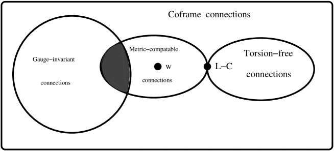
Figure 1: The different connections are depicted by the interior points of the rectangle. The bold points denote the Weitzenböck and the Levi-Civita connections. The gray area represents the gauge-invariant metric-compatible connections.

The standard Levi-Civita connection is invariant under arbitrary non-restricted variations of the coframe. This connection is a basis construction of the Riemannian geometry and consequently of the Einstein gravity theory.

We have derived an alternative family of connections which are invariant under restricted local variations of the coframe field. The variations themselves have to satisfy the equations

$$K_{[abc]}=0\,,\qquad K^{m}{}_{am}=0\,.$$ (3.24)

Due to (3.6) this is a system of eight first order partial differential equations for six enters of the antisymmetric matrix $X_{\alpha\beta}$. This is very similar to the standard Maxwell system for the electromagnetic field strength. We will examine the system (3.24) in section 5. But first we will give a gravity model corresponding to these gauge connections.

4 Coframe field models

4.1 Action and field equation

The Lagrangian of a gauge invariant gravity model has to respect the gauge transformations (3.4) restricted by (3.24). Starting with invariant fields of metric and connection, such Lagrangian can be constructed straightforwardly. Namely, we can take the standard Einstein-Hilbert Lagrangian calculated on our gauge invariant connections instead of the Levi-Civita connections

$${\cal{A}}=\int R\Big{(}\Gamma_{ab}{}^{c}\Big{)}\sqrt{-g}\,d^{4}x\,.$$ (4.1)

Moreover, since our connection is asymmetric, we can also consider the terms quadratic in torsion and non-metricity as acceptable additions to the Lagrangians. All such terms are of the same physical dimensions so they have to be involved with free dimensionless coefficients. This way we come to a rather complicated Lagrangian of MAG [22].

In our case, however, all the geometric quantities are constructed only from the coframe components and their first order derivatives. This fact simplifies very much the most general Lagrangian we are seeking for. Observe that the Einstein-Hilbert Lagrangian (4.1) can be rewritten as a linear combination of the first order derivatives of the coframe components plus a total derivative term. Also the torsion and non-metricity tensors are linear in the first order derivatives of the coframe. Consequently, the most general Lagrangian can be given by a linear combination of terms which are quadratic in the first order derivatives of the coframe.

A most general coframe Lagrangian can be straightforwardly constructed from the exterior derivative of the coframe components $\vartheta^{\alpha}{}_{[i,j]}$,

$$d\vartheta^{\alpha}=\vartheta^{\alpha}{}_{[i,j]}dx^{i}\wedge dx^{j}\,.$$ (4.2)

Equivalently, we can use the components $\vartheta^{\alpha}{}_{[i,j]}$ directly to deal with the tensorial expression

$$C_{ij}{}^{k}=e_{\alpha}{}^{k}\vartheta^{\alpha}{}_{[i,j]}\,,\qquad C_{ijk}=\eta_{\alpha\beta}\vartheta^{\alpha}{}_{k}\vartheta^{\beta}{}_{[i,j]}\,.$$ (4.3)

Now it is enough to consider the possible quadratic combinations of $d\vartheta^{\alpha}$ or, equivalently, of $C_{ij}{}^{k}$. In this way, a general quadratic coframe action takes the known form [15], [24]

$${}^{\tt(cof)}{\cal{A}}=\frac{\kappa}{2}\int\rho_{1}L_{1}+\rho_{2}\,L_{2}+\rho_{3}\,L_{3}\,,$$ (4.4)

where $\kappa$ is a coupling constant of dimension $1/\ell^{2}$, $\rho_{i}$ are free dimensionless parameters, while the “elementary” Lagrangian densities are defined as

$$L_{1} = d\vartheta^{\alpha}\wedge*d\vartheta_{\alpha},$$ (4.5)

$$L_{2} = (d\vartheta_{\alpha}\wedge\vartheta^{\alpha})\wedge*(d\vartheta_{\beta}\wedge\vartheta^{\beta}),$$ (4.6)

$$L_{3} = (d\vartheta_{\alpha}\wedge\vartheta^{\beta})\wedge*(d\vartheta_{\beta}\wedge\vartheta^{\alpha})\,.$$ (4.7)

The action (4.4) can be rewritten in a compact form

$${}^{\tt(cof)}{\cal{A}}=\frac{\kappa}{2}\int d\vartheta_{\alpha}\wedge*H^{\alpha}=\frac{\kappa}{2}\int C_{ijk}H^{ijk}\,\sqrt{-g}\,dx^{4}\,,$$ (4.8)

where

$$H^{ijk}=\rho_{1}\,C^{ijk}+3\rho_{2}C^{[ijk]}+\rho_{3}\Big{(}C^{ijk}-2\,C^{im}{}_{m}g^{jk}\Big{)}\,.$$ (4.9)

The corresponding 1-form is

$$H^{\alpha}=\frac{1}{2}\,H_{ijk}\vartheta^{\alpha}{}_{k}dx^{i}\wedge dx^{j}\,.$$ (4.10)

To make physics on the coframe background we have to involve a Lagrangian of a matter field $\psi$. We do not specify the tensorial or spinorial content of this field. Consequently,

$${}^{\tt(mat)}{\cal{A}}=\int L(\psi,\nabla_{\Gamma}\psi,g)\,,$$ (4.11)

where the integrand is a 4-form density. The covariant derivative in (4.11) has to be taken with respect to the same connection $\Gamma$ which is involved in the coframe Lagrangian. Consequently, also ${}^{(m)}{\cal{A}}$ involves the coframe components. Apply now the variation of the total Lagrangian

$${\cal{A}}={}^{\tt(cof)}A+{}^{\tt(mat)}A$$ (4.12)

with respect to the coframe field. We come to the coframe field equation which has a compact form in exterior calculus notation [24]

$$d*H^{\alpha}={}^{\tt(cof)}\Sigma^{\alpha}+{}^{\tt(mat)}\Sigma^{\alpha}\,,$$ (4.13)

where the right hand side involves the energy-momentum currents (3-form) of the coframe and the matter fields. These quantities are related to the energy-momentum tensors $T^{ij}$ in a regular way

$$\Sigma^{\alpha}=(1/6)\,T^{ij}\,\vartheta^{\alpha}{}_{i}\,\epsilon_{jklm}dx^{k}\wedge dx^{l}\wedge dx^{m}\,.$$ (4.14)

The standard Einstein-Hilbert action of GR is not completely distinct from the coframe action (4.4). Indeed, the term $R\sqrt{-g}$ can be rewritten as a total derivative plus squares of first order derivatives of the metric. Let us substitute $g_{ij}=\eta_{\alpha\beta}\vartheta^{\alpha}{}_{i}\vartheta^{\beta}{}_{j}$ and neglect with the total derivative. We remain with a scalar expression which is quadratic in the coframe components. Since all such type expressions are encoded in (4.4), there is a coframe Lagrangian with a special set of parameters is equivalent (up to a total derivative) to the standard Hilbert-Einstein Lagrangian. On the level of the field equations, we have here no more than the standard GR reformulated in the coframe variables. The explicit calculations [15] give the special (Einstein) choice of parameters

$$\rho_{1}=0\,,\qquad\rho_{2}=-1/2\,,\qquad\rho_{3}=1$$ (4.15)

Consequently, up to a total derivative, the Hilbert-Einstein action takes the form

$$\int R\sqrt{-g}\,{\rm vol}=\int\Big{(}-\frac{1}{2}\,L_{2}+\,L_{3}\Big{)}\,.$$ (4.16)

Note that although the energy-momentum tensor of the coframe field is defined also in this case, it cannot be identified as an energy-momentum tensor of gravity. Such identification quite often appears in literature, because one does not take into account a hidden symmetry of the coframe action. For (4.16), the action (4.4) is local Lorentz invariant. This symmetry, however, is not preserved for the coframe energy-momentum tensor expression.

4.2 Gauge invariant coframe Lagrangian

Let us examine now the behavior of the general coframe action (4.4) under the local Lorentz transformations (3.4). Using (4.16) we rewrite (up to a total derivative)

$$\int{}^{\tt{(cof)}}L=\int\Big{[}\rho_{1}L_{1}+(\rho_{2}+\frac{1}{2}\rho_{3})\,L_{2}\Big{]}+\rho_{3}\int R\sqrt{-g}\,{\rm vol}\,.$$ (4.17)

With respect to the transformations (3.4), this expression changes as

$$\delta\int{}^{\tt{(cof)}}L = \int\Big{[}\rho_{1}\delta L_{1}+(\rho_{2}+\frac{1}{2}\rho_{3})\delta L_{2}\Big{]}$$ (4.18)

$$= \int C_{ijk}\Big{[}2\rho_{1}K^{ijk}+(2\rho_{2}+\rho_{3})K^{[ijk]}\Big{]}\sqrt{-g}\,{\rm vol}\,.$$

Since the variations $K^{ijk}$ are independent, the action is invariant if and only if the following invariance condition holds

$$2\rho_{1}K^{ijk}+(2\rho_{2}-\rho_{3})K^{[ijk]}=0\,.$$ (4.19)

This algebraic equation has to be satisfied identically (for arbitrary coframe fields), thus we have three solutions to (4.19) of basically different types:

(i) ”The teleparallel equivalent of GR”

A first solution to (4.19) can be taken as

$$\rho_{1}=0\,,\qquad 2\rho_{2}+\rho_{3}=0\,.$$ (4.20)

Since the tensor $K^{ijk}$ is arbitrary now, the coframe Lagrangian with (4.20) is invariant under arbitrary Lorentz transformations. Consequently, six degrees of freedom of the coframe field are unphysical while the rest ten degrees are equivalent to the metric tensor. The underlining geometry for such coframe model is precisely Riemannian and not teleparallel as it is claimed sometimes. The fact that the coframe Lagrangian is expressed by the torsion of the Weitzenböck connection does not mean a lot, specially in view of the formula (2.10), which express the Levi-Civita connection by the Weitzenböck one.

The coframe reformulation of GR can serve as a useful technical tool, for instance for search of new solutions in GR [20] or for its Hamiltonian formulation [17]. It cannot change however the main features of GR. In particular, the so-called teleparallel energy-momentum tensors of gravitational field are no more than the pseudo-tensors of the standard GR.

(ii) The teleparallel gravity model.

Another solution to (4.19) is

$$K^{ijk}=0\,,\qquad\rho_{1}\neq 0\,.$$ (4.21)

Substituting into (3.6) we obtain $X_{\alpha\beta,i}=0$, thus only global (rigid) Lorentz transformations of the coframe field are admissible. Consequently, if a coframe is given at a point, it is also given on the whole manifold. Such teleparallel geometry is described by the Weitzenböck connection. Consequently, precisely the model (4.21) (and only this model) has to be refereed to as a teleparallel gravity model. Indeed only the Lagrangians with $\rho_{1}\neq 0$ do not have any local non-trivial group of transformations. This is in a complete correspondence to the flat teleparallel geometry.

With a non-zero parameter $\rho_{1}$, the coframe field equation (4.13) has spherical symmetric solutions of the type [19]

$$\vartheta^{\alpha}=\left(\frac{r}{r_{o}}\right)^{A}dx^{\alpha}\,,$$ (4.22)

where $A$ is a function of the parameters $\rho_{i}$. The corresponding metric does not have the Newtonian behavior at infinity. Consequently, the teleparallel model cannot serve for description of $4D$ gravitational field.

(iii) A model alternative to GR

The last solution to (4.19) is

$$K^{[ijk]}=0\qquad\rho_{1}=0\,,\qquad 2\rho_{2}-\rho_{3}\neq 0\,,$$ (4.23)

The first equation here is a first order partial differential equation for the matrix $X_{\alpha\beta}$. Thus, in contrast to the previous cases, we are dealing now with dynamical local Lorentz transformations.

For the coframe models with a zero parameter $\rho_{1}$, the field equation (4.13) has a unique static spherical-symmetric solution of a ”diagonal form” [19] :

$$\vartheta^{0}=\frac{1-m/2\rho}{1+m/2\rho}\,dx^{0}\,,\qquad\vartheta^{i}=\left(1+\frac{m}{2\rho}\right)^{2}\,dx^{i}\,,$$ (4.24)

where $i=1,2,3$. This coframe corresponds to the Schwarzschild metric in the isotropic coordinates.

Another justification for the condition $\rho_{1}=0$ comes from consideration of the first order approximation to the coframe field model [21]. In this case, the coframe variable is reduced to a sum of symmetric and antisymmetric matrices. It means that, in linear approximation, we can treat the coframe field as a system of two independent fields. It is natural to require all the field-theoretic constructions, i.e. the action, the field equation and the energy-momentum tensor, to accept the same separation to two independent expression. A remarkable fact that such separation (free field limit) appears if and only if $\rho_{1}=0$.

Consequently we have derived the equation

$$K^{[ijk]}=0\,,$$ (4.25)

as an invariance condition for a viable gravity field model. This is in an addition to the pure geometrical consideration given in the previous section.

4.3 Gauge invariant matter Lagrangian

We turn now to the second constrain $K^{m}{}_{im}=0$. Distinctly, it comes from the symmetry a generic matter Lagrangian. When the matter field $\psi$ is minimally coupled to gravity, its Lagrangian involves the covariant derivatives taken with respect to some connection

$${}^{(m)}L=L(\psi,\nabla_{\Gamma}\psi,g)\,.$$ (4.26)

Since the matter fields themselves are invariant under coframe transformations, also the connection $\Gamma$ has to be invariant. In other words,

$$\delta({}^{(m)}L)=0\quad{\rm yields}\quad\delta\Gamma_{ijk}=0\,.$$ (4.27)

In the case of a variety of connections the following problem emerges [29]: To what connection the matter field is really coupled? A natural answer can be proposed: The proper connection is this one which is already involved in the gravity sector of the model. In other words: The symmetries of the gravity and the matter sectors have to be conformed.

We continue now with our alternative model (4.23). Since the gravity sector is already restricted with the requirement $K_{[ijk]}=0$, it is natural to require the matter sector to respect this condition. This way we come to the family of connections (3.17) which are invariant under the local Lorentz transformations satisfied

$$K^{m}{}_{im}=0\,.$$ (4.28)

Consequently, the equations (3.24) emerge as the invariance conditions for the total action of a matter field coupling minimally to gravity.

5 Maxwell-compatible connection

5.1 Invariance conditions on the flat space

Let us examine now what physical meaning can be given to the invariance conditions

$$K_{[ijk]}=0\,,\qquad K^{m}{}_{im}=0\,.$$ (5.1)

Recall that the tensor $K_{ijk}$ depends on the derivatives of the Lorentz parameters $X_{\alpha\beta}$ and on the components of the coframe field

$$K_{ijk}=\frac{1}{2}\,\vartheta^{\alpha}{}_{k}\Big{(}X_{\alpha\beta,j}\vartheta^{\beta}{}_{i}-X_{\alpha\beta,i}\vartheta^{\beta}{}_{j}\Big{)}\,.$$ (5.2)

Thus, in fact, we have in (5.1), two first order partial differential equations for the entries of an antisymmetric matrix $X_{\alpha\beta}$. Let us construct from this matrix an antisymmetric tensor $F_{ij}$

$$F_{ij}=X_{\mu\nu}\vartheta^{\mu}{}_{i}\vartheta^{\nu}{}_{j}\,,\qquad X_{\mu\nu}=F_{ij}e_{\mu}{}^{i}e_{\nu}{}^{j}\,.$$ (5.3)

Substituting into (5.2), we derive

$$K_{ijk} = F_{k[i,j]}-\frac{1}{2}\,X_{\alpha\beta}\Big{[}(\vartheta^{\alpha}{}_{k}\vartheta^{\beta}{}_{i})_{,j}-(\vartheta^{\alpha}{}_{k}\vartheta^{\beta}{}_{j})_{,i}\Big{]}$$ (5.4)

$$= F_{k[i,j]}-F_{km}C_{ij}{}^{m}-\frac{1}{2}(F_{mi}\stackrel{{\scriptstyle{\rm o}}}{{\Gamma}}{\!}_{kj}{}^{m}-F_{mj}\stackrel{{\scriptstyle{\rm o}}}{{\Gamma}}{\!}_{ki}{}^{m})\,.$$

Consequently, the first equation from (5.1) takes the form

$$F_{[ij,k]}=\frac{2}{3}(C_{ij}{}^{m}F_{km}+C_{jk}{}^{m}F_{im}+C_{ki}{}^{m}F_{jm})\,,$$ (5.5)

while the second equation from (5.1) is rewritten as

$$F^{i}{}_{j,i}=-2F^{i}{}_{m}C_{ij}{}^{m}+F_{kj}g^{ki}{}_{,i}+F_{mj}g^{ki}\stackrel{{\scriptstyle{\rm o}}}{{\Gamma}}{\!}_{ki}{}^{m}-F_{mi}g^{ki}\stackrel{{\scriptstyle{\rm o}}}{{\Gamma}}{\!}_{kj}{}^{m}\,.$$ (5.6)

Observe first a significant approximation to (5.5—5.6). If the right hand sides in both equations are neglected, the equations take the form of the ordinary Maxwell equations for the electromagnetic field in vacuum —

$$F_{[ij,k]}=0\,,\qquad F^{i}{}_{j,i}=0\,.$$ (5.7)

In the coframe models, the gravity is modeled by a variable coframe field, i.e., by nonzero values of the quantities $\stackrel{{\scriptstyle{\rm o}}}{{\Gamma}}{\!}_{ij}{}^{k}$. Consequently, the right hand sides of (5.5—5.6) can be viewed as curved space additions, i.e., as the gravitational corrections to the electromagnetic field equations. In the flat spacetime, when a suitable coordinate system is chosen, these corrections are identically equal to zero. Consequently, in the flat spacetime, the invariance conditions (5.1) take the form of the vacuum Maxwell system.

5.2 Invariance conditions on a curved space

On a curved manifold, the standard Maxwell equations are formulated in a covariant form. Let us show that our system (5.5—5.6) is already covariant. We rewrite (5.4) as

$$K_{ijk}=\frac{1}{2}(F_{ki,j}-F_{km}\stackrel{{\scriptstyle{\rm o}}}{{\Gamma}}{\!}_{ij}{}^{m}-F_{mi}\stackrel{{\scriptstyle{\rm o}}}{{\Gamma}}{\!}_{kj}{}^{m})-\frac{1}{2}(\,\,i\longleftrightarrow j\,\,)\,.$$ (5.8)

Consequently,

$$K_{ijk}=F_{k[i;j]}\,,$$ (5.9)

where the covariant derivative (denoted by the semicolon) is taken relative to the Weitzenböck connection. Consequently, the system (5.5—5.6) takes the covariant form

$$F_{[ij;k]}=0\,,\qquad F^{i}{}_{j;i}=0\,.$$ (5.10)

These equations are literally the same as the electromagnetic sector field equations of the Maxwell-Einstein system. The crucial difference is encoded in the type of the covariant derivative. In the Maxwell-Einstein system, the covariant derivative is taken relative to the Levi-Civita connection, while, in our case, the corresponding connection is of Weitzenböck. Observe that, due to our approach, the Weitzenböck connection is rather natural in (5.10). Indeed, since the electromagnetic-type field describes the local change of the coframe field, it should itself be referred only to the global changes of the coframe. As we have shown, such global transformations correspond precisely to the teleparallel geometry with the Weitzenböck connections.

6 Gravity corrections to the Coulomb-type field

6.1 Gravity-electromagnetic coupling

The coupling between the electromagnetic and the gravitational field is an age-old problem. It is already related to the first observable prediction of GR about the bending of light rays of stars in the gravitational field of the Sun. The electromagnetic and gravitational effects are of rather different orders of magnitude. However, the increasing precision of modern experimental techniques gives rise to the hope that the appropriate form of the coupling can soon be determined.

In particular, we have in this context two independent but closely related problems:

• Does the gravitational field of a charged massive source depend on the electric charge?

• Does the electromagnetic field of a charged massive source depend on the mass?

From a certain philosophical point of view (“Everything has an influence on everything else”) the answer on both questions has to be positive.

In classical (non-relativistic) physics, the both answers are negative: The Newton force of attraction is independent on the charges, also the Coulomb force is not sensitive to the masses.

6.2 Gravity-electromagnetic coupling in GR

In the framework of GR, the coupling between the electromagnetic field and gravity is managed by the electromagnetic action itself

$$S(g,F)=-\frac{\lambda_{0}}{4}\int F_{ij}F^{ij}\sqrt{-g}\,d^{4}x\,,$$ (6.1)

where $\lambda_{0}$ is a coupling constant. When the actions of the gravitational and the matter fields are added to (6.1), the variation with respect to the metric yields the Einstein field equation (without cosmological constant)

$$R_{ij}-\frac{1}{2}\,Rg_{ij}=\frac{8\pi G}{c^{3}}\Big{(}{}^{\tt(em)}T_{ij}+{}^{\tt(mat)}T_{ij}\Big{)}\,.$$ (6.2)

Here the electromagnetic energy-momentum tensor ${}^{\tt(em)}T_{ij}$ and the matter energy-momentum tensor ${}^{\tt(mat)}T_{ij}$ are the sources of the gravitational field. The action (6.1) yields the electromagnetic field equation of the form

$$F_{[ij;k]}=0\,,\qquad F^{i}_{j;i}=J_{j}\,,$$ (6.3)

where the semicolon is used for the covariant derivative taken relative to the Levi-Civita connection. The dependence of the metric is encoded here in the index raising procedure and in the covariant derivatives.

The static spherical-symmetric solution to the Einstein-Maxwell system (6.2, 6.3) is given by the Reissner-Nordström metric

$$ds^{2}=\big{[}1-\lambda(r)\big{]}dt^{2}-\big{[}1-\lambda(r)\big{]}^{-1}dr^{2}-r^{2}d\Omega^{2},$$ (6.4)

with

$$\lambda(r)=\frac{2m}{r}-\frac{q^{2}}{r^{2}}\,,$$ (6.5)

and the Coulomb potential

$$A_{o}=\frac{Q}{r}\,.$$ (6.6)

Here $m=GM/c^{2}$ and $q^{2}=GQ^{2}/(4\pi\varepsilon_{0}c^{4})$ describes a mass $M$ with an electric charge $Q$. Consequently, in the Einstein-Maxwell system, the gravitational field depends on the charge of the source. The electromagnetic field of a pointwise source remains the same as in the flat spacetime, i.e., it is independent on the mass of the charge.

6.3 Mass corrections to the Coulomb-type field

Let us look for a static spherically symmetric solution to our electromagnetic-type equations (5.10). We start with a spherically symmetric solution in a vacuum coframe model (4.4) with the parameter $\rho_{1}=0$. We will use the isotropic coordinates $\{x^{\hat{i}}\,,\,{\hat{i}}=1,2,3\}$ with the isotropic radius

$$\rho=\sqrt{\delta_{{\hat{i}}{\hat{j}}}x^{\hat{i}}x^{\hat{j}}}=\sqrt{x^{2}+y^{2}+z^{2}}\,.$$ (6.7)

Recall that we identify the gravity variable with the coframe field defined up to an infinitesimal Lorentz transformation. It is equivalent to the metric field. Since the field equation (4.13) involves free parameters $\rho_{2}$ and $\rho_{3}$, it is alternative to GR. Although, the spherically symmetric gravity solution turns out to be the same. In particular, such solution can be taken in the form of a “diagonal” coframe [19]

$$\vartheta^{0}=\varphi(\rho)\,dx^{0}\,,\qquad\vartheta^{{\hat{i}}}=\psi(\rho)\,dx^{{\hat{i}}}\,,$$ (6.8)

where

$$\varphi(\rho)=\frac{1-m/2\rho}{1+m/2\rho}\,,\qquad\psi(\rho)=\left(1+\frac{m}{2\rho}\right)^{2}\,.$$ (6.9)

The non-zero components of the corresponding metric tensor are

$$g_{00}=-\varphi^{2}\,,\qquad g_{{\hat{i}}{\hat{i}}}=\psi^{2}\,,$$ (6.10)

while the line element is

$$ds^{2}=-\varphi^{2}c^{2}dt^{2}+\psi^{2}(dx^{2}+dy^{2}+dz^{2})\,.$$ (6.11)

Recall that (6.11) with (6.9) substituted is no more than the standard Schwarzschild line element in isotropic coordinates.

The nonzero components of the Weitzenböck connection (2.8) corresponding to the coframe (6.8) are

$$\stackrel{{\scriptstyle{\rm o}}}{{\Gamma}}{\!}_{0{\hat{i}}}{}^{0}=\frac{\varphi^{\prime}}{\varphi}\,\frac{x^{\hat{m}}}{\rho}\delta_{{\hat{i}}{\hat{m}}}\,,\qquad\stackrel{{\scriptstyle{\rm o}}}{{\Gamma}}{\!}_{{\hat{i}}{\hat{j}}}{}^{\hat{k}}=\frac{\psi^{\prime}}{\psi}\,\frac{x^{\hat{m}}}{\rho}\,\delta^{\hat{k}}_{\hat{i}}\delta_{{\hat{j}}{\hat{m}}}\,.$$ (6.12)

Consequently, the independent nonzero components of the Weitzenböck torsion tensor are

$$C_{0{\hat{i}}}{}^{0}=\frac{\varphi^{\prime}}{2\varphi}\,\frac{x^{\hat{m}}}{\rho}\delta_{{\hat{i}}{\hat{m}}}\,,\qquad C_{{\hat{i}}{\hat{j}}}{}^{\hat{k}}=\frac{\psi^{\prime}}{2\psi}\,\frac{x^{\hat{m}}}{\rho}(\delta_{{\hat{j}}{\hat{m}}}\delta^{\hat{k}}_{\hat{i}}-\delta_{{\hat{i}}{\hat{m}}}\delta^{\hat{k}}_{\hat{j}})\,.$$ (6.13)

The suitable ansatz for electromagnetic-type field of a pointwise charge can be taken as

$$F_{0}{}^{\hat{i}}=x^{\hat{i}}f(\rho)\,,\qquad F_{0{\hat{i}}}=\delta_{{\hat{i}}{\hat{m}}}x^{\hat{m}}f(\rho)\psi^{2}\,.$$ (6.14)

The first Maxwell-type equation $F_{[ij;k]}=0$ is satisfied identically when (6.13) and (6.14) are substituted. Indeed,

$$F_{[0{\hat{j}},{\hat{k}}]} = \frac{1}{3}(F_{0{\hat{j}},{\hat{k}}}-F_{0{\hat{k}},{\hat{j}}})$$ (6.15)

$$= \delta_{{\hat{j}}{\hat{m}}}(x^{\hat{m}}f\psi^{2})_{,{\hat{k}}}-\delta_{{\hat{k}}{\hat{m}}}(x^{\hat{m}}f\psi^{2})_{,{\hat{j}}}=0\,,$$

while

$$C_{0{\hat{j}}}{}^{m}F_{{\hat{k}}m}+C_{{\hat{j}}{\hat{k}}}{}^{m}F_{0m}+C_{{\hat{k}}0}{}^{m}F_{{\hat{j}}m}$$

$$\qquad=\frac{f\psi^{2}}{2}\left(\frac{\varphi^{\prime}}{\varphi}+\frac{\psi^{\prime}}{\psi}\right)\frac{x^{\hat{m}}x^{\hat{n}}}{\rho}(\delta_{{\hat{k}}{\hat{m}}}\delta_{{\hat{j}}{\hat{n}}}-\delta_{{\hat{k}}{\hat{n}}}\delta_{{\hat{j}}{\hat{m}}})=0\,.$$ (6.16)

The other components of the equation are zero because of (anti)symmetry and independence of time.

As for the second Maxwell-type equation $F^{i}{}_{j;i}=0$, we observe that for $j\neq 0$ both sides vanish. For $j=0$, we substitute (6.13) and (6.14) into (5.6) to obtain

$$f^{\prime}\rho+3f=f\rho\left(\frac{\varphi^{\prime}}{\varphi}-\frac{\psi^{\prime}}{\psi}\right)\,.$$ (6.17)

This equation is straightforward integrated to

$$f=\frac{Q}{\rho^{3}}\,\frac{\varphi}{\psi}=\frac{Q}{\rho^{3}}\,\frac{1-m/2\rho}{(1+m/2\rho)^{3}}\,,$$ (6.18)

where $Q$ is a constant of integration. Consequently, the non-zero field components are

$$F_{0}{}^{\hat{i}}=x^{\hat{i}}\frac{Q}{\rho^{3}}\,\frac{1-m/2\rho}{(1+m/2\rho)^{3}}\,.$$ (6.19)

The Coulomb-type force acted on a test charge $q$ (of a small mass) takes the form

$$F=\frac{Qq}{\rho^{2}}\,\frac{1-m/2\rho}{(1+m/2\rho)^{3}}\,.$$ (6.20)

The ordinary Cartesian radius $r$ is related to the isotropic radius $\rho$ as

$$r=\rho\left(1+\frac{m}{2\rho}\right)^{2}\,.$$ (6.21)

Hence

$$\rho=\frac{r-m+\sqrt{r^{2}-2mr}}{2}\approx r\left(1-\frac{m}{r}\right)\,.$$ (6.22)

Observe that the isotropic coordinates are defined only for $r>2m$. Consequently, the modernized Coulomb force takes the form

$$F=\frac{Qq}{r^{2}}\,\left(1-\frac{m^{2}}{4\rho^{2}}\right)\,.$$ (6.23)

Finally, in the Cartesian coordinates, the mass-correction terms take the form

$$F = Qq\,\frac{r-2m+\sqrt{r^{2}-2mr}}{4(r+\sqrt{r^{2}-2mr})^{3}}$$ (6.24)

$$= \frac{Qq}{r^{2}}\,\left(1-\frac{m^{2}}{4r^{2}}-\frac{m^{3}}{2r^{3}}+\cdots\right)\,.$$

Observe the complicated form of the solution in the standard polar coordinates. In fact, the choice of the isotropic coordinates can be viewed as a method to solve the differential equation $F^{i}{}_{j;i}=0$ exactly. Unfortunately, this method is restricted to $r>2m$.

Figure 2: The graphs represent the dependence of the force $F$ on $\rho/m$ and $r/m$ correspondingly relative to the Coulomb force (the top lines). In both cases $F$ is given in the units of $Qq/m^{2}$.

We depict the dependence of the force $F$ on the distances $\rho$ and $r$ on Fig. 2. The graphs start from $\rho=m/2$ and $r=2m$ which are the minimal possible value. The deviation from the Coulomb values appears only for small distances $\rho,r\sim m$. The maximal value of the force between two charged particles predicts as

$$F\approx 0.15\,{Qq}/{m^{2}}\,.$$ (6.25)

For two electrons, it gives $F\approx 0.76\cdot 10^{86}N$.

7 Outline of the model

7.1 “Gauge geometry”

We construct a complete class of connections linear in the first order derivatives of the coframe field. It involves the standard Levi-Civita connection and the flat Weitzenböck connection. For special choices of parameters, the torsion free and the metric compatible sub-families of connections emerge. Our main output is the identification of a sub-family of connections which are invariant under restricted local Lorentz transformations. The corresponding conditions are a set of eight first order equations. In the first order approximations the rotations are described by an antisymmetric matrix. In this case, the set of invariance conditions turns out to be the standard vacuum Maxwell system.

7.2 Field equations

We consider a Lagrangian of the matter-coframe system

$$L=^{(cof)}L(\vartheta^{\alpha},d\vartheta^{\alpha})+^{(mat)}L(\psi,d\psi,\vartheta^{\alpha})\,.$$ (7.1)

In the standard consideration, the arbitrary variation of the coframe field is assumed. The corresponding coframe field equation is [24]

$$d*{\mathcal{F}}^{\alpha}={\mathcal{T}}^{\alpha}\,,$$ (7.2)

with the energy-momentum 3-form of the coframe-matter system ${\mathcal{T}}=^{(cof)}{\mathcal{T}}+^{(mat)}{\mathcal{T}}$ in its right hand side. Consequently (7.2) represents a system of 16 independent equations. It can be covariantly decomposed to ten symmetric and six antisymmetric equations.

$$\vartheta^{(\beta}\wedge d*{\mathcal{F}}^{\alpha)} = \vartheta^{(\beta}\wedge{\mathcal{T}}^{\alpha)}\,$$ (7.3)

$$\vartheta^{[\beta}\wedge d*{\mathcal{F}}^{\alpha]} = \vartheta^{[\beta}\wedge{\mathcal{T}}^{\alpha]}\,,$$ (7.4)

Consider the pure coframe system, and restrict to the viable case $\rho_{1}=0$. The explicit calculations, see [18], show that both sides of (7.4) involve the leading coefficient $2\rho_{2}+\rho_{3}$. Consequently, for $2\rho_{2}+\rho_{3}=0$, only ten independent field equations (7.3) remain. Certainly, this symmetric system is equivalent to Einstein equation. In this case, the coframe field is defined only up to arbitrary Lorentz transformations. For the alternative models with $2\rho_{2}+\rho_{3}\neq 0$, (7.3-7.4) is a well posed system of 16 hyperbolic PDE for 16 independent variables. The coframe field is defined uniquely (up to global transformations).

In the approach proposed in the current paper, only the symmetric variations of the coframe field are independent. The antisymmetric variations are constrained by the system (5.10). Since the variation derivative of the Lagrangian is covariantly decomposed to the symmetric and antisymmetric parts, only one field equation, namely the symmetric one, (7.3), is derived from the symmetric variation of the action. The second field equation comes from the invariance of the Lagrangian. Consequently our system of equations includes 16 independent equations for 16 independent variables

$$\vartheta^{(\beta}\wedge d*{\mathcal{F}}^{\alpha)}=\vartheta^{(\beta}\wedge{\mathcal{T}}^{\alpha)}\,$$ (7.6)

$$F_{[ij;k]}=0\,,\qquad F^{i}{}_{j;i}=0\,.$$

The first (“gravitational”) equation has to give a class of orthonormal coframes, i.e., a solution that valid up to arbitrary transformations of the coframe. . The second (“electromagnetic”) equation has to define uniquely (up to global transformations) the field of local rotations. Although, the well-posedness of the system (7.6-7.6) requires a special consideration, it is rather reasonable. Indeed:

(i) In the first order approximation [21], the coframe field is decomposed to a sum of symmetric and antisymmetric fields. For $\rho_{1}=0$, also the system of field equations is separated — (7.6) involves only the symmetric part, while (7.4) describes the dynamics of the antisymmetric part. Moreover, in this approximation, (7.4) takes the form $\square F_{ij}=0$, which is a consequence of (7.6).

(ii) For a spherical-symmetric ansatz, (7.6) is equivalent to the vacuum Einstein equation, i.e., determines uniquely a class of orthonormal coframes. When the solution is substituted in (7.6) also the field $F_{ij}$ is determined uniquely (see the previous section).

(iii) The equation (7.6) involves the torsion tensor $C_{ijk}$ only linearly. Thus, it can be viewed as a linear combination of the derivatives $F_{ij,k}$. When these combinations are substituted into (7.6), the corresponding equation is a system of second order quasi-linear hyperbolic PDE for $F_{ij}$.

7.3 Pure “gravity” sector

Let the local Lorentz rotations $X_{\alpha\beta}$ (and, consequently, their approximations $F_{ij}$) are assumed to be independent on a point. In this case, the field equations (7.6) are satisfied. The remain 10 equations (7.6) is an under-defined system for 16 independent components of the coframe field. The metric tensor, however, is defined uniquely. In particular, with a mentioned restriction $\rho_{1}=0$, the system has a unique spherical-symmetric solution which corresponds to the Schwarzschild metric.

Moreover, the coframe field model for gravity has even some advantage relative to the standard metric GR. It is well known that an energy-momentum tensor cannot be constructed covariantly from the metric tensor and its first order derivatives. Consequently, the energy of a gravity field cannot be defined in GR. Alternatively, for a coframe field, the corresponding tensor is defined [24]. This tensor is not local Lorentz in Varian and so cannot be prolongated into the standard metric GR. However, in the model proposed here, the arbitrary local Lorentz transformations are not acceptable. Moreover, these transformations are governed by their own field equations.

7.4 Pure “electromagnetic” sector

Let the coframe field be defined up to a local pseudo-rotation. Thus the metric is defined uniquely. Moreover, let a representative coframe be chosen. The set of invariance conditions now is a system of eight first order equations for six independent variables $L_{\alpha\beta}$. In fact, we have here a linear field model for $L_{\alpha\beta}$, which turns to a non-linear field model for $X_{\alpha\beta}$, where

$$L_{\alpha\beta}=\eta_{\alpha\beta}+X_{\alpha\beta}+\mathcal{O}(X^{2})\,.$$ (7.7)

A similar non-linear extension of electrodynamics based on orthonormal tensor was recently discussed [33]. It can give an alternative to the Born-Infeld electrodynamics, which turns recently to a popular model in strings theory.

Recall, that in the current paper we consider only the first order approximation of the pseudo-orthonormal tensor $L_{\alpha\beta}$. The corresponding invariance conditions are

$$K_{[ijk]}=0\,,\qquad K^{m}{}_{im}=0\,,$$ (7.8)

or, after a redefinition of the variables,

$$F_{[ij;k]}=0\,,\qquad F^{m}{}_{i;m}=0\,,$$ (7.9)

where the covariant derivative is taken relative to the flat Weitzenböck connection. For a holonomic coframe field, these equations take the form of the standard Maxwell system

$$F_{[ij,k]}=0\,,\qquad F^{m}{}_{i,m}=0\,.$$ (7.10)

Observe the main properties of the derived field equations:

• The (approximated) Maxwell-type system is not introduced by hand, but emerges in a natural way as a set of invariance condition for a geometry and for a viable Lagrangian.

• The complete field equation is nonlinear, what is in a correspondence with the string model consequences.

• The spherical symmetric solution is bounded near the Schwarzschild radius. Further off, it is close to the Coulomb field.

• It is well known that in the models with an asymmetric connection, the torsion contribution is an obstacle for the standard definition of the potentials, $F_{ij}=\partial_{i}A_{j}-\partial_{j}A_{i}$. For torsion of a restricted type, the potentials can be defined, however, as

  $$F_{ij}=\partial_{i}A_{j}-\partial_{j}A_{i}+2T^{k}{}_{ij}A_{k}$$ (7.11)

  and the modified gauge transformations are acceptable [34].

• In the standard Maxwell theory a charge is not connected to a mass. Thus, unphysical massless charges are not forbidden. In our construction, the field of pseudo-rotations can be degenerate only in the singularities of the coframe field (metric). With this requirement, the charges are necessary massive. Certainly, the field of rotations can be regular in the whole space even the coframes are singular. In this case, we have uncharged masses.

• A nonzero constant field $F_{ij}$ is another unphysical solution of the Maxwell system, which is usually removed by the boundary conditions. The modified field equation (7.9) does not have such a solution.

• In the first order approximation, the coframe can be covariantly decomposed in a sum of its symmetric and antisymmetric parts. In this case, the difference between coordinate and coframe indices can be neglected. Consequently, we can write

  $$\vartheta_{ij}=\vartheta_{(ij)}+\vartheta_{[ij]}=g_{ij}+\frac{1}{\beta}F_{ij}\,.$$ (7.12)

  The free parameter $\beta$ has a dimension of a field strength. Note that the structure of (7.12) is similar to a combination appearing in the Born-Infeld electrodynamics, where $\beta$ is a maximal electromagnetic field. From our spherical symmetric solution $\beta\approx m^{2}/(0.15{q})$. At this stage, it is only a speculation because $\beta$ has sense only in higher order approximations.

• In this paper, we have considered only the vacuum case. A complete model has to include a Lagrangian for fermions. Due to Fock and Dirac, the fermionic Lagrangian on a curved space is constructed with the spin connections. A remarkable fact that this Dirac connection is proportional to the flat connection of Weitzenböck. Consequently, the covariant derivative is the same as in (7.9).

• Qualitatively, the coframe structure in our model can be described as a ”paramagnetic substance”. The gravitational sector establishes the coframe at every point, i.e., the lengths of four covectors and the angles between them. The coframes do not interact with one another and are randomly oriented. The metric on the manifold is defined uniquely. The electromagnetic-type sector orders the coframes attached at different points in a smooth coframe field. Different type of ordering correspond to different connections from the six parametric family described above.

8 Results

On a manifold endowed with a coframe (vierbein, tetrad) field, we constructed a most general linear asymmetric connection. Besides the torsion-free and metric-compatible connections, we identified a subset of Maxwell-compatible connections. The vacuum Maxwell-type equations emerges as the conditions for invariance of the connection under Lorentz transformations of the coframe.

We derive the same equations as invariant conditions for a viable coframe Lagrangian which has the Schwarzschild solution even being alternative to GR.

In our approach, the curved space Maxwell-type equations emerges formally the same as in the standard Maxwell-Einstein system. The covariant derivatives is different, however, in proposed model they are taken relative to the flat connection. The result is a different behavior of the electromagnetic field near the Schwarzschild radius. Moreover, the model predicts an upper bound for the electromagnetic-type field of a source with given charge and mass. Note that although the gravitational field of a charged source remains independent on the charge, it is only a result of the approximation used. Already in the second approximation, the metric tensor is not invariant under the first order approximate Lorentz transformations and a quadratic correction, $F_{i}{}^{m}F_{mj}$, emerges in the metric tensor.

In the current paper, we have treated only the vacuum case. The problem of the sources for the proposed Maxwell-type field requires additional investigations. In particular, they can appear from a viable modification of Dirac field on a coframe background.

References

References

- [1] A. Ashtekar, Phys. Rev. D 36, 1587 (1987).
- [2] S. Deser and C. J. Isham, Phys. Rev. D 14, 2505 (1976).
- [3] J. M. Nester and R. S. Tung, Phys. Rev. D 49, 3958 (1994) [arXiv:gr-qc/9401002].
- [4] S. Deser and P. van Nieuwenhuizen, Phys. Rev. D 10, 411 (1974).
- [5] P. G. Bergmann, V. de Sabbata, G. T. Gillies and P. I. Pronin, International School of Cosmology and Gravitation: 15th Course: Spin in Gravity: Is it Possible to Give an Experimental Basis to Torsion?, Erice, Italy, 13-20 May 1997.
- [6] P. Van Nieuwenhuizen, Phys. Rept. 68, 189 (1981).
- [7] W. Kummer, “Progress and problems in quantum gravity,” arXiv:gr-qc/0512010.
- [8] A. Perez and C. Rovelli, Phys. Rev. D 73, 044013 (2006)
- [9] H. F. M. Goenner, Living Rev. Rel. 7, 2 (2004).
- [10] R. Bluhm and A. Kostelecky, arXiv:hep-th/0412320.
- [11] K. Hayashi and T. Shirafuji, Phys. Rev. D 19, 3524 (1979)
- [12] J. Nitsch and F. W. Hehl, Phys. Lett. B 90, 98 (1980);
- [13] F. Mueller-Hoissen and J. Nitsch, Phys. Rev. D 28, 718 (1983);
- [14] E. W. Mielke, Annals Phys. 219, 78 (1992);
- [15] U. Muench, F. Gronwald and F. W. Hehl, Gen. Rel. Grav. 30, 933 (1998);
- [16] R. S. Tung and J. M. Nester, Phys. Rev. D 60, 021501 (1999);
- [17] M. Blagojevic and M. Vasilic, Class. Quant. Grav. 17, 3785 (2000);
- [18] Y. Itin and S. Kaniel, J. Math. Phys. 41, 6318 (2000)
- [19] Y. Itin, Int. J. Mod. Phys. D 10, 547 (2001)
- [20] Y. N. Obukhov and J. G. Pereira, Phys. Rev. D 67, 044016 (2003)
- [21] Y. Itin, J. Math. Phys. 46 12501 (2005),
- [22] F. W. Hehl, J. D. McCrea, E. W. Mielke and Y. Neeman, Phys. Rept. 258, 1 (1995);
- [23] F. W. Hehl and A. Macias, Int. J. Mod. Phys. D 8, 399 (1999)
- [24] Y. Itin, Class. Quant. Grav. 19, 173 (2002);
- [25] Y. Itin, Gen. Rel. Grav. 34, 1819 (2002);
- [26] Y. Itin, J. Phys. A 36, 8867 (2003)
- [27] J.A. Schouten, Ricci-Calculus, An Introduction to Tensor Analysis and its Geometrical Applications (2nd ed., Springer-Verlag, New York, 1954).
- [28] Y. Itin, “Coframe geometrical structures: Linear coframe connections”, to appear.
- [29] F.W. Hehl and Yu.N. Obukhov, Lecture Notes in Physics Vol. 562 (Springer: Berlin, 2001) pp. 479-504.
- [30] F. W. Hehl, P. Von Der Heyde, G. D. Kerlick and J. M. Nester, Rev. Mod. Phys. 48, 393 (1976).
- [31] I. L. Shapiro, Phys. Rept. 357, 113 (2001)
- [32] R. T. Hammond, Rept. Prog. Phys. 65, 599 (2002).
- [33] B. Coll, Annales Fond. Broglie 29, 247 (2004)
- [34] S. Hojman, M. Rosenbaum, M. P. Ryan and L. C. Shepley, Phys. Rev. D 17, 3141 (1978).