Quantum geometry and black hole entropy: inclusion of distortion and rotation

Abstract

Equilibrium states of black holes can be modelled by isolated horizons. If the intrinsic geometry is spherical, they are called type I while if it is axi-symmetric, they are called type II. The detailed theory of geometry of quantum type I horizons and the calculation of their entropy can be generalized to type II, thereby including arbitrary distortions and rotations. The leading term in entropy of large horizons is again given by 1/4th of the horizon area for the same value of the Barbero-Immirzi parameter as in the type I case. Ideas and constructions underlying this extension are summarized.

I Introduction

Since the work by Bekenstein, Hawking, et al. in the early seventies on black hole thermodynamics, proposals have been made of various sorts for a microscopic explanation of black hole entropy. Prominent among these is the loop quantum gravity calculation of black hole entropy published in 2000 abk (see also abck and earlier work cited therein). The present work aev aims at an extension of this calculation: the previous calculation restricted itself to the case in which the intrinsic geometry of the black hole horizon is spherically symmetric – the “type I” case. We will refer to this previous calculation as the “type I” calculation. In the present work, we extend the calculation to the inclusion of rotation and distortion of the horizon compatible with axisymmetry. This is referred to as the “type II” case.

Both of these calculations assume isolated horizon boundary conditions at the horizon. We will not go over the definition of isolated horizons here; it is sufficient to say that a horizon is called “isolated” if its intrinsic geometry is time-independent. Physically speaking, then, an isolated horizon represents a “black hole in equilibrium.” For further details, see for example abl ,ak .

II Classical phase space and tools

A key tool used in the extension of the calculation are certain multipoles defined for isolated horizons aepv :

$$I_{n}+iL_{n}:=-\int_{S}Y_{n,0}(\zeta)\Psi_{2}\,{}^{\scriptscriptstyle 2}\!\epsilon$$ (1)

where $S$ is a cross-section of the isolated horizon, $\,{}^{\scriptscriptstyle 2}\!\epsilon$ is the area $2$-form on $S$, and $(\zeta,\varphi)$ are the unique coordinates on $S$ in which the metric takes the standard form

$$q=R^{2}\left(\frac{1}{f(\zeta)}\mathrm{d}\zeta^{2}+f(\zeta)\mathrm{d}\varphi^{2}\right).$$ (2)

$\zeta$ takes values in $[-1,1]$ and $\varphi$ takes values in $\mathbb{R}/2\pi\mathbb{Z}$.

The most important property for us that these multipoles have is that they completely determine the intrinsic geometry of the horizon upto diffeomorphism. The plan is to come up with operators in the quantum theory corresponding to the multipoles which we will then use to characterize the quantum ensemble for which we calculate the entropy. The importance of the multipoles and area determining the intrinsic geometry upto diffeomorphism is that they thus determine the “macroscopic state” of the black hole and hence form a good set of observables for fully characterizing the ensemble.

The approach we are taking is to quantize the following phase space. Our basic variables are the Ashtekar-Barbero variables $({}^{\gamma}\!A_{a}^{i},{}^{\gamma}\Sigma_{ab}^{i})$ (throughout this presentation the conventions in al are used). We have an internal boundary which is $S^{2}\times\mathbb{R}$, and on this boundary we impose isolated horizon boundary conditions, and require this isolated horizon to be type II, have fixed multipoles $\mathring{I}_{n}$,$\mathring{L}_{n}$ and fixed area $a_{o}$. On this phase space, it turns out that one cannot simply use the naive symplectic structure

$$\Omega(\delta_{1},\delta_{2})=-\int_{M}\mathrm{Tr}(\delta_{1}{}^{\gamma}\!A\wedge\delta_{2}{}^{\gamma}\Sigma-\delta_{2}{}^{\gamma}\!A\wedge\delta_{1}{}^{\gamma}\Sigma)=\int_{M}\omega(\delta_{1},\delta_{2})$$ (3)

where $\omega$ is the symplectic current derived from the action of the theory. This is because such a symplectic structure is not preserved under time evolution.

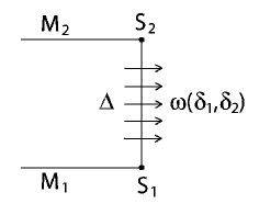
Figure 1: symplectic current escapes through the horizon

Figure 1 shows the cause of this lack of preservation: symplectic current is escaping across the horizon. More precisely, we have

$$\int_{M_{2}}\omega(\delta_{1},\delta_{2})=\int_{M_{1}}\omega(\delta_{1},\delta_{2})-\int_{\Delta}\omega(\delta_{1},\delta_{2})$$ (4)

The solution is to use the isolated horizon boundary conditions to rewrite the $\Delta$-integral as

$$\int_{\Delta}\omega(\delta_{1},\delta_{2})=\left(\oint_{S_{2}}-\oint_{S_{1}}\right)\alpha(\delta_{1},\delta_{2})$$ (5)

where $\alpha(\delta_{1},\delta_{2})$ is defined locally on $S_{1}$ and on $S_{2}$. (4) then becomes

$$\int_{M_{2}}\omega+\oint_{S_{2}}\alpha=\int_{M_{1}}\omega+\oint_{S_{1}}\alpha$$ (6)

so that

$$\Omega=\int_{M}\omega+\oint_{S}\alpha$$ (7)

will work as a definition of the symplectic structure that is invariant under time translations. As one might suspect, there is an ambiguity in the choice of $\alpha$. Nevertheless, there is a natural resolution to this ambiguity in the present context.

Before writing out explicitly the natural choice for $\alpha$, it will be convenient to introduce two $U(1)$ connections on the horizon $\Delta$. In our framework, as in abk , for simplicity we fix an internal vector field $r^{i}$ at the horizon and impose the partial gauge fixing condition that $e^{a}_{i}r^{i}$ be the unit spatial normal to the horizon. This reduces the gauge group at the horizon to $U(1)$. The connections ${}^{\gamma}V$ and $W$ we are about to define represent connections on this principal $U(1)$ subbundle. First we define

$${}^{\gamma}V:=\frac{1}{2}\hbox to0.0pt{\lower 6.45831pt\hbox{$\longleftarrow$}\hss}{{}^{\gamma}\!A}^{i}r_{i}$$ (8)

where the underarrow denotes pullback to $\Delta$. In terms of ${}^{\gamma}V$, the boundary condition reflecting that $\Delta$ is an isolated horizon takes the form

$$\mathrm{d}{}^{\gamma}V={}^{\gamma}\Psi_{2}\,{}^{\scriptscriptstyle 2}\!\epsilon={}^{\gamma}\Psi_{2}(8\pi\gamma)(\hbox to0.0pt{\lower 6.45831pt\hbox{$\longleftarrow$}\hss}{{}^{\gamma}\Sigma}\cdot r)$$ (9)

where ${}^{\gamma}\Psi_{2}:=\mathrm{Re}\Psi_{2}+\gamma\mathrm{Im}\Psi_{2}$.

We then define

$$W:={}^{\gamma}V+\frac{1}{4}(\mathring{f}^{\prime}-f^{\prime})\mathrm{d}\varphi-\frac{\gamma}{2}\omega$$ (10)

where $f$ and $\varphi$ are as in (2), $\omega$ is the rotation one-form on the horizon (see abl ), $\mathring{f}:=1-\zeta^{2}$, and the prime denotes derivative with respect to $\zeta$. In terms of $W$, the natural choice for $\alpha$ is

$$\alpha(\delta_{1},\delta_{2})=\frac{1}{8\pi G}\frac{a_{o}}{\gamma\pi}\delta_{1}W\wedge\delta_{2}W$$ (11)

so that our symplectic structure is given by

$$\Omega(\delta_{1},\delta_{2})=-\int_{M}\mathrm{Tr}(\delta_{1}{}^{\gamma}\!A\wedge\delta_{2}{}^{\gamma}\Sigma-\delta_{2}{}^{\gamma}\!A\wedge\delta_{1}{}^{\gamma}\Sigma)+\frac{1}{8\pi G}\frac{a_{o}}{\gamma\pi}\oint_{S}\delta_{1}W\wedge\delta_{2}W$$ (12)

It is also important to note that, in terms of $W$, the boundary condition (9) is now equivalent to a condition of the familiar type I form:

$$\mathrm{d}W=\left(-\frac{2\pi}{a_{o}}\right)(8\pi\gamma)(\hbox to0.0pt{\lower 6.45831pt\hbox{$\longleftarrow$}\hss}{{}^{\gamma}\Sigma}\cdot r)$$ (13)

(see abk and ack ).

III Quantization and entropy

The situation we see now is formally identical to the situation encountered in the type I calculation: we have a $U(1)$ connection $W$ describing the connection degrees of freedom at the horizon, and a surface term in the symplectic structure which is identical to the Chern-Simons surface term appearing in the type I case. Furthermore, the horizon boundary condition in terms of $W$ is the same boundary condition that appeared in the type I calculation.

We are therefore led to the same quantization scheme used in the type I case. Let us review the scheme. One first separates the phase space into bulk and surface phase spaces, and quantizes each separately – the bulk using standard loop quantum gravity techniques, and quantizing the surface theory as a Chern-Simons theory. We then tensor product the two resulting Hilbert spaces together, and impose the quantum version of boundary condition (13).

Finally we impose the constraints of GR to obtain the final physical Hilbert space.

As was done in the type I case, we define the relevant ensemble to include all horizon area eigenstates with area eigenvalue equal to $a_{0}$ plus or minus some tolerance $\delta$, all of these eigenstates being equally weighted. Since the ensemble is the same as in the type I calculation, the entropy is in fact the same. Thus, we again reproduce the Bekenstein Hawking entropy using the same value of the Barbero-Immirzi parameter used in the type I case.

IV Type II geometry operators

But if we wish to be more ambitious, gain a better intuition for the horizon geometry in terms of its type II character, or at least gain a more complete characterization of the ensemble just constructed, it is important to construct operators corresponding to quantities more directly related to the type II nature of the horizon. Let us begin by building operators at the level of the kinematical Hilbert space. At that level of the quantization we have the following picture.

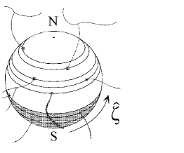
Figure 2: Behavior of $\hat{\zeta}$ eigenvalues

The kinematical Hilbert space is spanned by spin-network states. Each spin-network state may be visualized as a graph embedded in $3$-space, with verticies allowed to lie on the inner $2$-sphere boundary $S$. These vertices are referred to as “punctures.” The punctures are both the sources for the surface Chern-Simons theory, and the locations where horizon surface area is “concentrated” in discrete amounts. This is the physical picture.

In the present, type II case, we have a further basic structure entering the picture. At the classical level, given any $S^{2}$ cross-section $S$ of a type II isolated horizon with sufficiently generic multipoles, the axial symmetry field Lie-dragging the intrinsic geometry of $S$ is unique. The orbits of this symmetry field give us a foliation of $S$ into circular leaves; we call this foliation “axial” and denote it by “$\xi$”. $\xi$ is a pure gauge degree of freedom on the inner $2$-sphere boundary. That is, the group of diffeomorphisms acts transitively on the space of possible $\xi$’s.

To extract the physics of the situation in the quantum theory, we simply fix $\xi$. This may be thought of as “gauge-fixing.”

Regarding the legitimacy of this: It would be more satisfactory if the gauge-fixing could be done as true gauge fixing. The problem is that if one actually gauge fixes $\xi$ to be equal to some background $\xi_{0}$, that reduces the group of diffeomorphisms we divide out by at the quantum level. This reduction of the gauge group causes problems when we take into consideration the handling of certain extra structures necessary in the quantization of the surface phase space. In fact, the final entropy we calculate if we do this is ambiguous. Our viewpoint is that this problem is due to the fact that, by fixing $\xi$, we have broken diffeomorphism invariance, and diffeomorphism invariance is “sacred.”

Nevertheless, we need a fixed $\xi$ to build certain physical operators — so we fix one. There is no harm in doing this because in the physical Hilbert space one divides out by diffeomorphisms anyway: the choice of a fixed $\xi$ does not matter at that level. The most important operators we will build using $\xi$ are the multipole operators, operators which will carry over to the physical Hilbert space.

For convenience, let us furthermore introduce a coordinate $\zeta_{0}$ labelling the leaves of $\xi$. Nothing we do is going to depend on the choice of this coordinate; it is introduced merely for convenience.

Next, we introduce an operator corresponding to the preferred coordinate $\zeta$ introduced classically in (2). Classically, the $\zeta$ coordinate has the convenient property that it increases from South to North in proportion to area:

Figure 3: Classical $\zeta$ increases in proportion to area

$$\zeta(\zeta_{0}^{\prime})=-1+\frac{2a_{\zeta_{0}<\zeta_{0}^{\prime}}}{a_{S}}$$ (14)

So that we define

$$\hat{\zeta}(\zeta_{0}^{\prime})=-1+\frac{2\hat{a}_{\zeta_{0}<\zeta_{0}^{\prime}}}{\hat{a}_{S}}$$ (15)

where $\hat{a}_{\zeta_{0}<\zeta_{0}^{\prime}}$ is the area operator corresponding to the portion of $S$ defined by $\zeta_{0}<\zeta_{0}^{\prime}$.

As $\hat{\zeta}$ is an operator-valued function on the sphere, its eigenvalues may be thought of as functions on the sphere.

Let us gain a picture of the behavior of these eigenvalues. Given a spin-network state, recall area is concentrated at the punctures in discrete amounts. Consequently, the eigenvalues of $\hat{\zeta}$ jump discontinuously at leaves which contain punctures and everywhere else the eigenvalues are constant. This is represented in figure (2).

Next, we define an operator for $\Psi_{2}$. On the original classical phase space, the multipoles are fixed. One can show this means that $\Psi_{2}$ as a function of $\zeta$ is completely fixed. Specifically, if we set $4\pi R_{0}^{2}:=a_{o}$, the function is given by

$$\mathring{\Psi}_{2}(x)=-\frac{1}{R_{0}^{2}}\sum_{n}(\mathring{I}_{n}+i\mathring{L}_{n})Y_{n,0}(x),\quad\left(\mathring{\Psi}_{2}:[-1,1]\rightarrow\mathbb{C}\right)$$ (16)

That is, on the classical phase space, $\Psi_{2}=\mathring{\Psi}_{2}(\zeta)$. An obvious definition is then

$$\hat{\Psi}_{2}:=\mathring{\Psi}_{2}(\hat{\zeta})$$ (17)

Finally, we define the multipole operators. The basic definition for the multipoles is given by

$$I_{n}+iL_{n}=-\oint_{S}\Psi_{2}Y_{n,0}(\zeta)\,{}^{\scriptscriptstyle 2}\!\epsilon=-\frac{a_{S}}{2}\int_{-1}^{1}\Psi_{2}Y_{n,0}(\zeta)\mathrm{d}\zeta$$ (18)

One would like to simply take this expression directly over to the quantum theory. However, as it stands, there is a problem with the integrand. Because the $\hat{\zeta}$ eigenvalues depend on position in a discontinous manner at the punctures, the eigenvalues of $\mathrm{d}\hat{\zeta}$ will have $\delta$-functions at the punctures. But the other elements of the integrand, as they are functions of $\hat{\zeta}$, will be discontinuous at the punctures. Consequently, the meaning of the expression is ambiguous: we have delta functions multiplied into discontinous functions.

The way we choose to regularize is simply to replace the eigenvalues $\zeta$, which are discontinuous, with a family of smooth $\zeta_{i}$’s that converge to the physical $\zeta$ in the limit $i\rightarrow\infty$. We then take the limit $i\rightarrow\infty$:

$$\hat{I}_{n}+i\hat{L}_{n} = -\lim_{i\to\infty}\frac{\hat{a}_{S}}{2}\int_{-1}^{1}\mathring{\Psi}_{2}(\hat{\zeta}_{i})Y_{n,0}(\hat{\zeta}_{i})\mathrm{d}\hat{\zeta}_{i}$$ (19)

$$= \frac{\hat{a}_{S}}{a_{o}}\left(\mathring{I}_{n}+i\mathring{L}_{n}\right)$$

giving us the final expression for the multipole operators.

From this expression, it is easy to see, for example, that for the ensemble defined in the previous section the relative fluctuations in the multipoles will be equal to the relative fluctuations in the area. Furthermore, just as $\langle\hat{a}_{S}\rangle$ is within a fixed, small bound ($\delta$) of $a_{0}$, $\langle\hat{I}_{n}+i\hat{L}_{n}\rangle$ is within a fixed, small bound of $\mathring{I}_{n}+i\mathring{L}_{n}$ for each n. Thus we obtain a more complete characterization of the ensemble and the nature of the fluctuations being allowed.

V Summary

We have mapped the entropy calculation problem for the type II case to the type I case via an appropriate choice of variable $W$. In terms of this variable, the surface term in the symplectic structure is just Chern-Simons, and the relation between $W$ and the bulk variables is the same as in the type I case – that is, the appropriate “quantum boundary condition” we impose at the quantum level is still the same. Therefore we are able to do the quantization in the same manner as was done in the type I case, and get the same entropy.

The difference between the type I and type II cases lies in the physical interpretation of $W$. In the type I case, the concentrations of $\mathrm{d}W$ at punctures can be interpreted in terms of deficit angles (see abk ). In the type II case, on the other hand, in order to obtain a physical interpretation, we introduced the $\hat{\zeta}$ operator, $\hat{\Psi}_{2}$ operator, and multipole operators.

It is worthwhile to note how much of an extension the present work represents. The space of type II isolated horizons is infinite dimensional, encompassing the (finite dimensional) family of Kerr type isolated horizons as well as all possible distortions of such horizons compatible with axisymmetry. A vast range of astrophysically realistic black holes are therefore covered.

References

- (1) Ashtekar A, Baez J and Krasnov K 2000 “Quantum geometry of isolated horizons and black hole entropy” Adv. Theor. Math. Phys. 1 1-94
- (2) Ashtekar A, Baez J, Corichi A and Krasnov K 1998 “Quantum geometry and black hole entropy” Phys. Rev. Lett. 80 904-907
- (3) Ashtekar A, Engle J and Van Den Broeck C 2005 “Quantum horizons and black-hole entropy: inclusion of distortion and rotation” Class. Quantum Grav. 22 L27-L34
- (4) Ashtekar A, Beetle C and Lewandowski J 2001 “Mechanics of Rotating Isolated Horizons” Phys. Rev. D 64 044016
- (5) Ashtekar A, Krishnan B 2004 “Isolated and dynamical horizons and their applications” Living Rev. Rel. 7 10
- (6) Ashtekar A, Engle J, Pawlowski T and Van Den Broeck C 2004 “Multipole moments of isolated horizons” Class. Quantum Grav. 21 2549-70
- (7) Ashtekar A, Lewandowski J 2004 “Background independent quantum gravity: a status report” Class. Quantum Grav. 21 R53
- (8) Ashtekar A, Corichi A and Krasnov K 2000 “Isolated horizons: the classical phase space” Adv. Theor. Math. Phys. 3 419-478