The Futures of Bianchi type VII₀ cosmologies with vorticity

Abstract.

We use expansion-normalised variables to investigate the Bianchi type VII₀ model with a tilted $\gamma$-law perfect fluid. We emphasize the late-time asymptotic dynamical behaviour of the models and determine their asymptotic states. Unlike the other Bianchi models of solvable type, the type VII₀ state space is unbounded. Consequently we show that, for a general non-inflationary perfect fluid, one of the curvature variables diverges at late times, which implies that the type VII₀ model is not asymptotically self-similar to the future. Regarding the tilt velocity, we show that for fluids with $\gamma<4/3$ (which includes the important case of dust, $\gamma=1$) the tilt velocity tends to zero at late times, while for a radiation fluid, $\gamma=4/3$, the fluid is tilted and its vorticity is dynamically significant at late times. For fluids stiffer than radiation ($\gamma>4/3$), the future asymptotic state is an extremely tilted spacetime with vorticity.

1. Introduction

Much progess has been made recently in understanding spatially homogeneous (SH) cosmologies containing a perfect fluid with an equation of state $p=(\gamma-1)\rho$, where $\gamma$ is a constant. For the SH cosmologies known as the Bianchi models, the universe is foliated into space-like hypersurfaces (defined by the group orbits of the respective model) and the Einstein equations describe the evolution of these hypersurfaces [1, 2, 3, 4, 5, 6]. For these models there are two naturally defined time-like vectors: the unit vector field, $n^{\mu}$, normal to the group orbits, and the four-velocity, $u^{\mu}$, of the perfect fluid. When analysing the Bianchi models it is common to utilize $n^{\mu}$ as the preferred timelike vector field in the formalism, while the fluid velocity $u^{\mu}$ may or may not be aligned with $n^{\mu}$. If $u^{\mu}$ is not aligned with $n^{\mu}$, the model is called tilted, and non-tilted (or orthogonal) otherwise [7].

All of the non-tilted Bianchi models, except for the type IX model, have been studied in detail (see e.g., [2, 10]). For tilted Bianchi models the picture is less complete; the type II model was studied in [11], the type V model in [12, 13, 14, 15, 16], type VI₀ in [17, 18], types IV and VII_h in [19, 20], a subset of the type VI_h models in [19], and irrotational type VII₀ models were studied in [19]. In this paper we will use a dynamical systems approach and investigate the tilted type VII₀ models.

In the class of spatially homogeneous Bianchi models the type VII₀ model is a special, and particularly interesting, case. For Bianchi models containing a non-tilted perfect fluid, it was shown that the type VII₀ model experiences a self-similarity breaking at late times [21, 22] (see also [23, 24]). The irrotational models show the same behaviour [19]. The reason for this self-similarity breaking is because one of the curvature variables grows unbounded, which leads to an oscillation of the shear and the curvature variables with a frequency increasing with time. We will see that the same behaviour occurs for the fully tilted type VII₀ models; however, in this case there are two oscillations with different frequencies (one in the shear and curvature variables, and the other in the tilt velocity).

The investigation of the type VII₀ model is important for several reasons. First, the type VII₀ model is the most general spatially homogeneous model allowing for the flat Friedmann-Robertson-Walker (FRW) model as a special case (see Fig.1). Both the Bianchi type I model and the VII₀ generalise the flat FRW model; however, since the Bianchi type I perfect fluid model does not allow for tilt, only the Bianchi type VII₀ model can be used to investigate the effect of tilt on the evolution of the universe close to flatness. In addition, the type VII₀ model plays an important role in the Bianchi hierarchy (depicted in Fig.2). The higher up in the hierarchy, the more free parameters the model contains and thus the more ’general’ they are. Fig. 2 also shows the possible limits (solid arrows) of the various Lie algebras. For example, the type VII₀ is a special limit of both the ’most general’ type VIII and type IX models. In order to understand a particular Bianchi model, a complete understanding of all its descendants at the lower levels is needed. This implies that an understanding of the type VII₀ model is necessary for a full understanding of the two general semi-simple models (i.e., the type VIII and IX models).

Figure 1. The Bianchi generalisations of the closed ($k=1$), flat ($k=0$) and open ($k=-1$) FRW model.

Figure 2. The Bianchi Hierarchy: Solid arrows indicate Lie algebra contractions, or certain special limits of the Lie algebra parameters. Dashed lines indicate one-parameter families of non-isomorphic Lie algebras.

2. Equations of motion for the tilted VII₀ model

The Bianchi type VII₀ model has the Lie algebra of Killing vectors given by:

$$[{\mbox{\boldmath${\xi}$}}_{1},{\mbox{\boldmath${\xi}$}}_{2}]={\mbox{\boldmath${\xi}$}}_{3},\quad[{\mbox{\boldmath${\xi}$}}_{1},{\mbox{\boldmath${\xi}$}}_{3}]=-{\mbox{\boldmath${\xi}$}}_{2}.$$

This Lie algebra is solvable and in [19] a formalism for studying the tilted solvable Bianchi models was given. In this paper we will use this formalism to study the Bianchi type VII₀ model with full tilt.

In the dynamical systems approach we introduce expansion-normalised shear variables (bold variables are complex variables) $(\Sigma_{+},{\mbox{\boldmath${\Sigma}$}}_{\times},{\mathbb{\Sigma}}_{1})$ and the curvature variables $(A,\bar{N},{\bf N}_{\times})$. More specifically, $N^{a}_{~{}a}=2\sqrt{3}\bar{N}$ while ${\bf N}_{\times}$ consists of the trace-free part of $N_{ab}$. Moreover, for the type VII₀ model, $A=0$. Regarding the fluid, $\Omega$ is the expansion-normalised energy density and the tilt velocity is given by one real and one complex variable, $v_{1}$ and ${\bf v}=v_{2}+iv_{3}$. We note that the fluid in the Class A models has non-zero vorticity if and only if $N_{ab}v^{a}\neq 0$ [7], which implies that the type VII₀ model has vorticity if and only if ${\bf v}\neq 0$. It is also necessary to introduce the dimensionless time variable, $\tau$, defined by

(1) $$\frac{\mathrm{d}t}{\mathrm{d}\tau}=\frac{1}{H},$$

where $t$ is the cosmological time and $H$ is the Hubble scalar.

The equations of motion in [19] are given in terms of an arbitrary gauge function $\phi$. In terms of the above variables, the gauge transformation is given by

(2) $$\left({\bf N}_{\times},{\mbox{\boldmath${\Sigma}$}}_{\times},{\mbox{\boldmath${\Sigma}$}}_{1},{\bf v}\right) \mapsto \left(e^{2i\phi}{\bf N}_{\times},e^{2i\phi}{\mbox{\boldmath${\Sigma}$}}_{\times},e^{i\phi}{\mbox{\boldmath${\Sigma}$}}_{1},e^{i\phi}{\bf v}\right).$$

Several different gauges were proposed and discussed (including their advantages and disadvantages). In this paper we will adopt the ’F-gauge’ for which $\phi^{\prime}=0$. This still leaves us with an unspecified constant gauge freedom. The system of equations will therefore contain one more variable than the number of physical degrees of freedom. The physical properties of the system can be extracted by considering gauge independent quantites such as, for example, ${\mbox{\boldmath${\Sigma}$}}_{\times}{\bf N}^{*}_{\times}$ and ${\bf N}^{*}_{\times}{\bf v}^{2}$.

In the ’F-gauge’ ($\phi^{\prime}=0$) the equations of motion are:

(3) $$\Sigma_{+}^{\prime} = (q-2)\Sigma_{+}+{3}|{\mbox{\boldmath${\Sigma}$}}_{1}|^{2}-2|{\bf N}_{\times}|^{2}+\frac{\gamma\Omega}{2G_{+}}\left(-2v_{1}^{2}+|{\bf v}|^{2}\right)$$

(4) $${\mbox{\boldmath${\Sigma}$}}_{\times}^{\prime} = (q-2){\mbox{\boldmath${\Sigma}$}}_{\times}+\sqrt{3}{\mbox{\boldmath${\Sigma}$}}_{1}^{2}-2\sqrt{3}{\bf N}_{\times}\bar{N}+\frac{\sqrt{3}\gamma\Omega}{2G_{+}}{\bf v}^{2}$$

(5) $${\mbox{\boldmath${\Sigma}$}}^{\prime}_{1} = \left(q-2-3\Sigma_{+}\right){\mbox{\boldmath${\Sigma}$}}_{1}-\sqrt{3}{\mbox{\boldmath${\Sigma}$}}_{\times}{\mbox{\boldmath${\Sigma}$}}_{1}^{*}+\frac{\sqrt{3}\gamma\Omega v_{1}}{G_{+}}{\bf v}$$

(6) $${\bf N}_{\times}^{\prime} = \left(q+2\Sigma_{+}\right){\bf N}_{\times}+2\sqrt{3}{\mbox{\boldmath${\Sigma}$}}_{\times}\bar{N}$$

(7) $$\bar{N}^{\prime} = \left(q+2\Sigma_{+}\right)\bar{N}+2\sqrt{3}\mathrm{Re}\left({\mbox{\boldmath${\Sigma}$}}_{\times}^{*}{\bf N}_{\times}\right)$$

The equations for the fluid are

(8) $$\quad\Omega^{\prime} = \frac{\Omega}{G_{+}}\Big{\{}2q-(3\gamma-2)+\left[2q(\gamma-1)-(2-\gamma)-\gamma\mathcal{S}\right]V^{2}\Big{\}}\quad$$

(9) $$v_{1}^{\prime} = \left(T+2\Sigma_{+}\right)v_{1}-2\sqrt{3}\mathrm{Re}\left({\mbox{\boldmath${\Sigma}$}}_{1}{\bf v}^{*}\right)+\sqrt{3}\mathrm{Im}({\bf N}_{\times}^{*}{\bf v}^{2})$$

(10) $${\bf v}^{\prime} = \left(T-\Sigma_{+}-i\sqrt{3}\bar{N}v_{1}\right){\bf v}-\sqrt{3}\left({\mbox{\boldmath${\Sigma}$}}_{\times}+i{\bf N}_{\times}v_{1}\right){\bf v}^{*}$$

(11) $$V^{\prime} = \frac{V(1-V^{2})}{1-(\gamma-1)V^{2}}\left[(3\gamma-4)-\mathcal{S}\right]$$

where

$$q = 2\Sigma^{2}+\frac{1}{2}\frac{(3\gamma-2)+(2-\gamma)V^{2}}{1+(\gamma-1)V^{2}}\Omega$$

$$\Sigma^{2} = \Sigma_{+}^{2}+|{\mbox{\boldmath${\Sigma}$}}_{\times}|^{2}+|{\mbox{\boldmath${\Sigma}$}}_{1}|^{2}$$

$$\mathcal{S} = \Sigma_{ab}c^{a}c^{b},\quad c^{a}c_{a}=1,\quad v^{a}=Vc^{a},\quad$$

$$V^{2} = v_{1}^{2}+|{\bf v}|^{2},\quad$$

$$G_{+} = 1+(\gamma-1)V^{2},$$

(12) $$T = \frac{(3\gamma-4)(1-V^{2})+(2-\gamma)V^{2}\mathcal{S}}{1-(\gamma-1)V^{2}}.$$

These variables are subject to the constraints

(13) $$1 = \Sigma^{2}+|{\bf N}_{\times}|^{2}+\Omega$$

(14) $$0 = 2\mathrm{Im}({\mbox{\boldmath${\Sigma}$}}_{\times}^{*}{\bf N}_{\times})+\frac{\gamma\Omega v_{1}}{G_{+}}$$

(15) $$0 = i\mbox{\boldmath${\Sigma}$}_{1}\bar{N}+i{\mbox{\boldmath${\Sigma}$}}^{*}_{1}{\bf N}_{\times}+\frac{\gamma\Omega{\bf v}}{G_{+}}$$

The parameter $\gamma$ will be assumed to be in the interval $\gamma\in(0,2)$. The generalised Friedmann equation, eq.(13), yields an expression which effectively determines the energy density $\Omega$. The state vector will therefore be considered to be ${\sf X}=[\Sigma_{+},{\mbox{\boldmath${\Sigma}$}}_{\times},{\mbox{\boldmath${\Sigma}$}}_{1},{\bf N}_{\times},\bar{N},v_{1},{\bf v}]$ modulo the constraint equations (14) and (15). Thus the real dimension of the dynamical system is eight of which one is the remaining gauge freedom; i.e., the dimension of the physical state space is seven.

The dynamical system is invariant under the following discrete symmetries:

$$\phi_{1}: [\Sigma_{+},{\mbox{\boldmath${\Sigma}$}}_{\times},{\mbox{\boldmath${\Sigma}$}}_{1},{\bf N}_{\times},\bar{N},v_{1},{\bf v}]\mapsto[\Sigma_{+},{\mbox{\boldmath${\Sigma}$}}_{\times},{\mbox{\boldmath${\Sigma}$}}_{1},-{\bf N}_{\times},-\bar{N},-v_{1},-{\bf v}]$$

$$\phi_{2}: [\Sigma_{+},{\mbox{\boldmath${\Sigma}$}}_{\times},{\mbox{\boldmath${\Sigma}$}}_{1},{\bf N}_{\times},\bar{N},v_{1},{\bf v}]\mapsto[\Sigma_{+},{\sf u}^{2}{\mbox{\boldmath${\Sigma}$}}_{\times}^{*},-{\sf u}{\mbox{\boldmath${\Sigma}$}}_{1}^{*},{\sf u}^{2}{\bf N}_{\times}^{*},\bar{N},-v_{1},{\sf u}{\bf v}^{*}],~{}~{}{\sf u}\in S^{1}$$

$$\phi_{3}: [\Sigma_{+},{\mbox{\boldmath${\Sigma}$}}_{\times},{\mbox{\boldmath${\Sigma}$}}_{1},{\bf N}_{\times},\bar{N},v_{1},{\bf v}]\mapsto[\Sigma_{+},{\mbox{\boldmath${\Sigma}$}}_{\times},-{\mbox{\boldmath${\Sigma}$}}_{1},{\bf N}_{\times},\bar{N},v_{1},-{\bf v}].$$

These discrete symmetries imply that without loss of generality we can restrict the variables $\bar{N}\geq 0$ and $v_{1}\geq 0$. We also note that the free parameter ${\sf u}$ in $\phi_{2}$ is, in fact, the remaining gauge transformation.

2.1. Invariant Subspaces

In this analysis we will be concerned with the following invariant sets:

1. $T(VII_{0})$: The general tilted type VII₀ model with $\bar{N}^{2}-\left|{\bf N}_{\times}\right|^{2}>0$.

2. $T_{1}(VII_{0})$: The irrotational type VII₀ models defined by $\bar{N}^{2}-\left|{\bf N}_{\times}\right|^{2}>0$, ${\mbox{\boldmath${\Sigma}$}_{1}}={\bf v}=0$.

3. $F(VII_{0})$: The set of fixed points of $\phi_{2}$ (without loss of generality we can set ${\sf u}=1$) defined by $v_{1}=\mathrm{Im}({\mbox{\boldmath${\Sigma}$}}_{\times})=\mathrm{Re}({\mbox{\boldmath${\Sigma}$}}_{1})=\mathrm{Im}({\bf N}_{\times})=\mathrm{Im}({\bf v})=0$.

4. $B(VII_{0})$: Non-tilted Bianchi type VII₀ models with $\bar{N}^{2}-\left|{\bf N}_{\times}\right|^{2}>0$, $v_{1}={\bf v}=0$.

5. $T(II)$: The general tilted type II model given by $\bar{N}^{2}-\left|{\bf N}_{\times}\right|^{2}=0$.

6. $B(I)$: Type I: $\bar{N}={\bf N}_{\times}=V=0$.

7. $\partial T(I)$: “Tilted” vacuum type I: $\Omega=\bar{N}={\bf N}_{\times}=0$.

We note that the closure of the set $T(VII_{0})$ is given by:

(16) $$\overline{T(VII_{0})}=T(VII_{0})\cup T(II)\cup B(I)\cup\partial T(I).$$

Morever, in $\overline{T(VII_{0})}$ we have the bounds

(17) $$\Sigma_{+}^{2}+|{\mbox{\boldmath${\Sigma}$}}_{\times}|^{2}+|{\mbox{\boldmath${\Sigma}$}}_{1}|^{2}+\left|{\bf N}_{\times}\right|^{2}\leq 1,\quad v^{2}_{1}+|{\bf v}|^{2}\leq 1;$$

hence, all variables are bounded except for $\bar{N}$ (which can become arbitrary large).

2.2. Monotonic functions

There are three monotonic functions which are useful for our analysis:

(18) $$Z_{1} \equiv \alpha\Omega^{1-\Gamma},\quad\alpha=\frac{(1-V^{2})^{\frac{1}{2}(2-\gamma)}}{G_{+}^{1-\Gamma}V^{\Gamma}},\quad\Gamma=\frac{6}{7}\gamma,$$

$$Z_{1}^{\prime} = \left[2(1-\Gamma)q+(2+2\Gamma-3\gamma)+\Gamma\mathcal{S}\right]Z_{1}.$$

We note that (by the same trick as in [19])

$$2(1-\Gamma)q+(2+2\Gamma-3\gamma)+\Gamma\mathcal{S}$$

$$\geq\frac{1}{7}(14-15\gamma)(2\Sigma^{2}+|{\bf N}_{\times}|^{2})+\frac{\gamma\left[18(1-\gamma)+(10-9\gamma)V^{2}\right]}{7G_{+}}\Omega.$$

Thus $Z_{1}$ is monotonically increasing in $T(VII_{0})$ for $\gamma\leq 14/15$.

(19) $$Z_{2} \equiv \frac{\left(\bar{N}^{2}-|{\bf N}_{\times}|^{2}\right)^{n}\beta\Omega}{\left(1+n\Sigma_{+}\right)^{2(1+n)}},\quad\beta\equiv\frac{(1-V^{2})^{\frac{1}{2}(2-\gamma)}}{G_{+}},\quad n\equiv\frac{1}{4}(3\gamma-2)$$

$$Z_{2}^{\prime} = \frac{4}{1+n\Sigma_{+}}\Bigg{\{}\left(\Sigma_{+}+n\right)^{2}+(1-n^{2})|{\mbox{\boldmath${\Sigma}$}}_{\times}|^{2}+\frac{(1+n)(2-5n)}{2}|{\mbox{\boldmath${\Sigma}$}}_{1}|^{2}$$

$$\qquad+\frac{(1+2n)(1+n)\Omega}{6G_{+}}\left[2(1-n)v_{1}^{2}+(2-5n)|{\bf v}|^{2}\right]\Bigg{\}}Z_{2}.$$

$Z_{2}$ is monotonically increasing for the following subspaces: $T_{1}(VII_{0})$ for $0<\gamma<2$, and $T(VII_{0})$ for $0<\gamma\leq 6/5$.

(20) $$Z_{3} \equiv \frac{\left[\bar{N}|{\bf v}|^{2}+\mathrm{Re}({\bf N}_{\times}^{*}{\bf v}^{2})\right]^{2}}{(1-V^{2})^{2(2-\gamma)}\beta\Omega},$$

$$Z_{3}^{\prime} = 3(5\gamma-6)Z_{3}.$$

Thus $Z_{3}$ is monotonically decreasing ($\gamma<6/5$) or increasing ($6/5<\gamma$) in $T(VII_{0})\setminus T_{1}(VII_{0})$.

3. Qualitative analysis

The above monotonic functions allow us to obtain some results regarding the asymptotic behaviour of Bianchi type VII₀ universes:

Theorem 3.1.

For $0<\gamma<6/5$, all tilted Bianchi models (with $\Omega>0$, $V<1$) of type VII₀ are asymptotically non-tilted at late times.

Proof.

For $0<\gamma\leq 14/15$ we can use the monotonic function $Z_{1}$, which immediately gives the desired result. For $2/3<\gamma<6/5$, and using the monotonic function $Z_{3}$, we get $\bar{N}|{\bf v}|^{2}+\mathrm{Re}({\bf N}_{\times}^{*}{\bf v}^{2})\rightarrow 0$. Moreover, using $Z_{2}$, we get $\bar{N}\rightarrow\infty$ and hence $|{\bf v}|\rightarrow 0$. This implies that the solution asymptotically approaches the invariant subspace $T_{1}(VII_{0})$. The $T_{1}(VII_{0})$ analysis [19] can now be applied which shows that $v_{1}\rightarrow 0$. The theorem now follows. ∎

In fact, we believe that the type VII₀ models are asymptotically non-tilted for $0<\gamma<4/3$; however, this is not covered by this theorem.

Another important observation is the divergence of the variable $\bar{N}$ at late times. In fact, we firmly believe that:

Conjecture 3.2.

For a non-inflationary perfect fluid ($2/3<\gamma<2$) and any initial condition in $T(VII_{0})$ with $V<1$ and $\Omega>0$, we have that

$$\lim_{\tau\rightarrow+\infty}\left|\bar{N}\right|=\infty.$$

There are several results that support this conjecture. First, use of the monotonic function $Z_{2}$ immediately establishes this result for $T_{1}(VII_{0})$ and for $2/3<\gamma<6/5$ with general tilt (which includes the important case $\gamma=1$). Moreover, using $Z_{3}$ we have that for $6/5<\gamma$, $\bar{N}\rightarrow\infty$ or $V\rightarrow 1$. Second, a “local analysis” shows that the conjecture is true locally. And third, in our numerical analysis no other behaviour has been seen. In Appendix C some of the numerical plots are presented; in particular, we see that $M\equiv 1/\bar{N}\rightarrow 0$ for various values of $\gamma$.

3.1. Equilibrium points

3.1.1. $B(I)$: equilibrium points of Bianchi type I

1. $\mathcal{I}(I)$: $q=\tfrac{1}{2}(3\gamma-2)$, $\Omega=1$, $\Sigma_{+}={\mbox{\boldmath${\Sigma}$}}_{\times}={\mbox{\boldmath${\Sigma}$}}_{1}={\bf N}_{\times}=\bar{N}=V=0$
   Eigenvalues: $\tfrac{1}{2}(3\gamma-2)[\times 3]$, $-\tfrac{1}{2}(2-\gamma)[\times 4]$.
   The remaining equilibrium points of type I are all in $\partial T(I)$.

3.1.2. $T(II)$: equilibrium points of Bianchi type II

All of the equilibrium points in the set $T(II)$ are unstable. They are all given in [20] (in ’F-gauge’).

3.1.3. $T(VII_{0})$: equilibrium points of Bianchi type VII₀

Using the monotonic functions $Z_{3}$ and $Z_{2}$, it is possible to show that there are no equilibrium points in $T(VII_{0})$, apart from the following:

1. $\mathcal{L}^{\alpha}_{k}(VII_{0})$: $q=2$, $\Sigma_{+}=-1$, $\bar{N}=k=\text{constant}$, ${\mbox{\boldmath${\Sigma}$}}_{\times}={\mbox{\boldmath${\Sigma}$}}_{1}={\bf N}_{\times}=\Omega=0$, with the tilt velocities given by:

   1. $0<\gamma<2$, $v_{1}={\bf v}=0$.

   2. $0<\gamma<2$, $v_{1}=1$, ${\bf v}=0$.

   3. $0<\gamma<2$, $v_{1}=0$, $|{\bf v}|=1$.

   4. $\gamma=1$, $v_{1}=0$, $0<|{\bf v}|<1$.

2. $\mathcal{F}_{k}(VII_{0})$: $q=0$, $\bar{N}=k=\text{constant}$, $\Omega=1$, $\Sigma_{+}={\mbox{\boldmath${\Sigma}$}}_{\times}={\mbox{\boldmath${\Sigma}$}}_{1}={\bf N}_{\times}=V=0$, $\gamma=\frac{2}{3}$.
   Eigenvalues: $0$, $-2[\times 2]$, $-1\pm\sqrt{1-12k^{2}}[\times 2]$.
   This is an attracting set (for $\gamma=2/3$).

All of the equilibrium points in $\overline{T(VII_{0})}$, including the ones in the sets $T(II)$, $B(I)$, $\partial T(I)$, can be shown to be unstable into the future for $2/3<\gamma<2$.

3.2. Late time analysis

For the type VII₀ model it is convenient to solve constraint (15) to obtain an expression for ${\mbox{\boldmath${\Sigma}$}}_{1}$:

(21) $${\mbox{\boldmath${\Sigma}$}}_{1}=\frac{i\gamma\Omega}{G_{+}\left(\bar{N}^{2}-\left|{\bf N}_{\times}\right|^{2}\right)}\left(\bar{N}{\bf v}+{\bf N}_{\times}{\bf v}^{*}\right).$$

In the following we will introduce the variable

(22) $$M\equiv\frac{1}{\bar{N}}.$$

In light of conjecture 3.2, we have that $M\rightarrow 0$. In particular,

(23) $${\mbox{\boldmath${\Sigma}$}}_{1}=\frac{i\gamma M\Omega}{G_{+}\left(1-M^{2}\left|{\bf N}_{\times}\right|^{2}\right)}\left({\bf v}+M{\bf N}_{\times}{\bf v}^{*}\right)=M{\bf B},$$

where ${\bf B}$ is a bounded (complex) function.

Due to the oscillatory behaviour of the system, we introduce the following variables

(24) $${\mbox{\boldmath${\Sigma}$}}_{\times}+i{\bf N}_{\times} \equiv e^{2i\psi}{\bf X},$$

(25) $${\mbox{\boldmath${\Sigma}$}}_{\times}-i{\bf N}_{\times} \equiv e^{-2i\psi}{\bf Y},$$

(26) $${\bf v} \equiv e^{-i\theta}v_{2},$$

where

(27) $$\psi^{\prime} = \frac{\sqrt{3}}{M},$$

(28) $$\theta^{\prime} = \frac{\sqrt{3}}{M}\left\{v_{1}+\frac{1}{2}M\mathrm{Im}\left[(1+v_{1}){\bf X}e^{2i(\theta+\psi)}+(1-v_{1}){\bf Y}e^{2i(\theta-\psi)}\right]\right\}.$$

The angular variables $\psi$ and $\theta$ are introduced to take care of the rapid oscillation as $M\rightarrow 0$. We note that the variables $\psi$ and $\theta$ are not in synchronization since $v_{1}<1$. Hence, in general, we expect two different oscillations with different frequencies. The equation of motions for these variables are given in Appendix A. In this case we can explicitly see how the oscillatory terms enter into the equations of motion. Moreover, we note that both of these rapid oscillations are observable; e.g., by considering the scalars:

$$S_{1} = ({\mbox{\boldmath${\Sigma}$}}_{\times}+i{\bf N}_{\times})({\mbox{\boldmath${\Sigma}$}}_{\times}^{*}+i{\bf N}_{\times}^{*})=e^{4i\psi}{\bf X}{\bf Y}^{*},$$

$$S_{2} = ({\mbox{\boldmath${\Sigma}$}}_{\times}^{2}+{\bf N}_{\times}^{2})({\bf v}^{*})^{4}=e^{4i\theta}{\bf X}{\bf Y}v_{2}^{4}.$$

3.3. Reduced System

The idea is that as $M\rightarrow 0$ at late times, the system of equations effectively reduces to a much simpler system of equations. In Appendix A the idea behind this reduction is explained in more detail; by introducing new variables this reduction of the full system is manifest as $M\rightarrow 0$. This method was also used in the previous analyses of the type VII₀ model [21, 22, 19] with success. Moreover, in Appendix B a linear analysis is given to put bounds on solutions of the reduced system with respect to the full system.

Therefore we assume that $M\rightarrow 0$, which implies that ${\mbox{\boldmath${\Sigma}$}}_{1}\rightarrow 0$. Consequently, from above we have that all oscillatory terms effectively cancel. Defining

(29) $$\sigma_{1} \equiv \left|{\bf N}_{\times}\right|^{2}+\left|{\mbox{\boldmath${\Sigma}$}}_{\times}\right|^{2}=\frac{1}{2}\left(|{\bf X}|^{2}+|{\bf Y}|^{2}\right),$$

(30) $$\sigma_{2} \equiv 2\mathrm{Im}\left({\mbox{\boldmath${\Sigma}$}}_{\times}{\bf N}_{\times}^{*}\right)=-\frac{1}{2}\left(|{\bf X}|^{2}-|{\bf Y}|^{2}\right),$$

the system given by eqs.(83-89) effectively reduces to the following system:

(31) $$\Sigma_{+}^{\prime} = (Q-2)\Sigma_{+}-\sigma_{1}+\frac{\gamma\Omega}{2G_{+}}\left(-2v_{1}^{2}+v_{2}^{2}\right)$$

(32) $$\sigma_{1}^{\prime} = 2(Q+\Sigma_{+}-1)\sigma_{1}$$

(33) $$M^{\prime} = -\left(Q+2\Sigma_{+}\right)M$$

(34) $$\Omega^{\prime} = \frac{\Omega}{G_{+}}\Big{\{}2Q-(3\gamma-2)+\left[2Q(\gamma-1)-(2-\gamma)-\gamma\mathcal{S}\right]V^{2}\Big{\}}$$

(35) $$v_{1}^{\prime} = \left(T+2\Sigma_{+}\right)v_{1}$$

(36) $$v_{2}^{\prime} = (T-\Sigma_{+})v_{2}$$

where

(37) $$Q = 2\Sigma^{2}_{+}+\sigma_{1}+\frac{1}{2}\frac{(3\gamma-2)+(2-\gamma)V^{2}}{1+(\gamma-1)V^{2}}\Omega,$$

(38) $$V^{2}\mathcal{S} = \left(-2v_{1}^{2}+v_{2}^{2}\right)\Sigma_{+}.$$

These variables are subject to the constraint

(39) $$1 = \Sigma^{2}_{+}+\sigma_{1}+\Omega.$$

Furthermore, $\sigma_{2}$ is determined from

$$\sigma_{2}=-\frac{\gamma\Omega v_{1}}{G_{+}},$$

which gives the bound

(40) $$\sigma_{1}\geq\frac{\gamma\Omega|v_{1}|}{G_{+}}.$$

Using the constraint (39) we can solve for $\sigma_{1}$ or $\Omega$.

3.3.1. Monotonic functions for the reduced system

By the same trick as in Appendix A, monotonic functions of the reduced system will at sufficiently late times also be monotonic for the full system. It is therefore useful to list some of the monotonic functions for the reduced system.

$$R_{1} \equiv \frac{\beta\Omega}{\sigma_{1}^{m}(1-m\Sigma_{+})^{2(1-m)}},\quad m=\frac{1}{2}(4-3\gamma),$$

$$R_{1}^{\prime} = \frac{2}{1-m\Sigma_{+}}\left[(\Sigma_{+}-m)^{2}+\frac{m(1-m)(2-m)|{\bf v}|^{2}\Omega}{G_{+}}\right]R_{1},$$

which is monotonically increasing for $2/3<\gamma<4/3$ if ${\bf v}\neq 0$, and for $2/3<\gamma<2$ if ${\bf v}=0$.

$$R_{2} \equiv \frac{v_{1}|{\bf v}|^{2}}{(1-V^{2})^{\frac{3}{2}(2-\gamma)}},$$

$$R_{2}^{\prime} = 3(3\gamma-4)R_{2},$$

which is monotonically decreasing or increasing for $\gamma<4/3$ and $\gamma>4/3$, respectively.

$$R_{3} \equiv \beta\Omega,$$

(41) $$R_{3}^{\prime} = \left[2\Sigma_{+}^{2}+\frac{(4-3\gamma)}{G_{+}}\left[(1-V^{2})(1-\Omega)+\gamma V^{2}\right]\right]R_{3},$$

which is monotonically increasing for $\gamma\leq 4/3$.

3.3.2. Equilibrium points for the reduced system

$\widetilde{P_{1}}$: $\Sigma_{+}=\sigma_{1}=M=v_{1}=v_{2}=0$, $\Omega=1$, $Q=\frac{1}{2}(3\gamma-2)$, $2/3<\gamma<2$.
Eigenvalues:

$$-\frac{1}{2}(3\gamma-2),\quad-(4-3\gamma)[\times 3],\quad-\frac{3}{2}(2-\gamma).$$

$\widetilde{P_{2}}$: $\Sigma_{+}=-\frac{1}{2}(3\gamma-4)$, $\sigma_{1}=\frac{3(2-\gamma)[(3\gamma-4)-v_{1}^{2}(5\gamma-4)]}{4(1-v_{1}^{2})}$, $M=v_{2}=0$, $\Omega=\frac{3(2-\gamma)G_{+}}{2(1-v_{1}^{2})}$, $Q=\frac{1}{2}(3\gamma-2)$, $0\leq v_{1}\leq\frac{3\gamma-4}{5\gamma-4}$, $4/3<\gamma<2$.
Eigenvalues:

$$0,\quad-3(4-3\gamma),\quad-\frac{3}{2}(2-\gamma),\quad-\frac{(2-\gamma)}{4}\left[1\pm\sqrt{1-\frac{4[(3\gamma-4)+v_{1}^{2}(5\gamma-4)]}{1-(\gamma-1)v_{1}^{2}}}\right].$$

$\widetilde{P_{3}}$: $\Sigma_{+}=M=0$, $\sigma_{1}=\frac{2(v_{2}^{2}-2v_{1}^{2})}{3(1-v_{1}^{2}+v_{2}^{2})}$, $\Omega=\frac{3+v_{1}^{2}+v_{2}^{2}}{3(1-v_{1}^{2}+v_{2}^{2})}$, $Q=1$, $\gamma=\frac{4}{3}$, $0\leq(2+3v_{1})v_{1}\leq v_{1}^{2}+v_{2}^{2}<1$.
Eigenvalues:

$$0[\times 2],\quad-1,\quad-\frac{1}{2}\left(1\pm\sqrt{1-\frac{16\left[2v_{1}^{2}(1-v_{1}^{2})+v_{2}^{2}(2-v_{2}^{2})\right]}{(1-v_{1}^{2}+v_{2}^{2})(3-V^{2})}}\right).$$

$\widetilde{P_{4}}$: $\Sigma_{+}=M=0$, $\sigma_{1}=\frac{1-3v_{1}^{2}}{3(1-v_{1}^{2})}$, $v_{2}=\sqrt{1-v_{1}^{2}}$, $\Omega=\frac{2}{3(1-v_{1}^{2})}$, $Q=1$, $0\leq v_{1}\leq 1/3$, $2/3<\gamma<2$.
Eigenvalues:

$$0,\quad-\frac{2(3\gamma-4)}{2-\gamma},\quad-1,\quad-\frac{1}{2}\left(1\pm i\sqrt{3+12v_{1}^{2}}\right).$$

4. Late time behaviour

Theorem 4.1.

For all tilted Bianchi models of type VII₀ with a perfect fluid stiffer than radiation ($4/3<\gamma<2$) and where the fluid has non-zero vorticity (${\bf v}\neq 0$), the fluid will asymptotically approach a state of extreme tilt; i.e., $\lim_{\tau\rightarrow\infty}V=1$.

Proof.

From the monotonic function $Z_{3}$ we have that $V\rightarrow 1$ or $\bar{N}\rightarrow\infty$. First, we assume that $\bar{N}\rightarrow\infty$. At sufficiently late times we can then use the reduced system. For $v_{1}\neq 0$, we use the function $R_{2}$ which is monotonically increasing at sufficiently late times. This shows that $V\rightarrow 1$. We assume, therefore, that $v_{1}=0$. For $v_{1}=0$ there is a monotonic function given by

$$R_{4}=\frac{\sigma_{1}|{\bf v}|^{2}}{(1-V^{2})^{(2-\gamma)}},\quad R_{4}^{\prime}=2\left[(3\gamma-4)\left(1+\frac{1-V^{2}}{2G_{+}}\Omega\right)+\Sigma_{+}^{2}\right]R_{4},$$

which again implies $V\rightarrow 1$. The theorem now follows. ∎

As summarized in Table 1, the tilt becomes extreme only in the case $\frac{4}{3}<\gamma<2$ for fluid with vorticity. In the case of zero vorticity, a very different tilt behaviour is observed; namely, the tilt tends to a non-extreme limit, as described by the equilibrium point $\widetilde{P}_{2}$ [19, 25].

Theorem 4.2.

Consider a perfect fluid Bianchi type VII₀ model with $2/3<\gamma\leq 4/3$ for which $\bar{N}\rightarrow\infty$. If $V<1$, then:

1. $\lim_{\tau\rightarrow\infty}(\Sigma_{+},V,\sigma_{1})=(0,0,0)$ for $2/3<\gamma<4/3$,

2. $\lim_{\tau\rightarrow\infty}\Sigma_{+}=0$ for $\gamma=4/3$.

Proof.

Use $R_{3}$. ∎

4.1. Decay rates for the case $\frac{2}{3}<\gamma<\frac{4}{3}$

By assuming an ansatz with coefficients and exponents to be determined, we obtain the decay rates when $\frac{2}{3}<\gamma<\frac{4}{3}$ as follows:

(42) $$\Sigma_{+} \approx-\frac{2\hat{\sigma}_{1}}{3\gamma-2}e^{-(4-3\gamma)\tau}+\hat{\Sigma}_{+}e^{-\frac{3}{2}(2-\gamma)\tau},$$

(43) $$\sigma_{1} \approx\hat{\sigma}_{1}e^{-(4-3\gamma)\tau},$$

(44) $$v_{1} \approx\hat{v}_{1}e^{-(4-3\gamma)\tau},$$

(45) $$v_{2} \approx\hat{v}_{2}e^{-(4-3\gamma)\tau},$$

(46) $$M \approx\hat{M}e^{-\frac{1}{2}(3\gamma-2)\tau}.$$

The angular variables are given asymptotically by:

(47) $$\psi \approx\hat{\psi}+\frac{2\sqrt{3}}{(3\gamma-2)\hat{M}}e^{\frac{1}{2}(3\gamma-2)\tau},$$

(48) $$\theta \approx\begin{cases}\hat{\theta},&2/3<\gamma<10/9\\ \hat{\theta}+\frac{\sqrt{3}\hat{v}_{1}}{\hat{M}}\tau,&\gamma=10/9\\ \hat{\theta}+\frac{2\sqrt{3}\hat{v}_{1}}{(9\gamma-10)\hat{M}}e^{\frac{1}{2}(9\gamma-10)\tau},&10/9<\gamma<4/3.\end{cases}$$

The meaning of the bifurcation value $\gamma=10/9$ is more clear if we calculate the fluid vorticity; in particular, to leading order we have:

(49) $$W^{a}W_{a}\propto e^{(9\gamma-10)\tau},\qquad W^{0}W_{0}\propto e^{3(5\gamma-6)\tau}.$$

We note that the bifurcation values for the vorticity and tilt at $\gamma=10/9$ and $\gamma=4/3$, respectively, coincide with with the values found in [26].

The Hubble-normalised Weyl scalars $\mathcal{W}_{1}$ and $\mathcal{W}_{2}$, defined by

(50) $$\mathcal{W}_{1}=\frac{C_{abcd}C^{abcd}}{48H^{4}}\,,\quad\mathcal{W}_{2}=\frac{C_{abcd}{}^{*}C^{abcd}}{48H^{4}}\,,$$

evolve as

$$\mathcal{W}_{1}+i\mathcal{W}_{2} \approx -\frac{12}{M^{2}}S_{1}$$

(51) $$\Rightarrow\quad(\mathcal{W}_{1},\mathcal{W}_{2}) \approx -\frac{12}{\hat{M}^{2}}\sqrt{\hat{\sigma}_{1}^{2}-\gamma^{2}\hat{v}_{1}^{2}}\,e^{6(\gamma-1)\tau}(\cos 2\psi_{2},\sin 2\psi_{2})\ ,$$

where $0\leq\hat{v}_{1}\leq\frac{\hat{\sigma}_{1}}{\gamma}$, $\hat{M}$ is the constant from the variable $M$, and $\psi_{2}$ is defined by $S_{1}=|S_{1}|e^{2i\psi_{2}}$. The angular variable $\psi_{2}$ is related asymptotically to the variable $\psi$ via $\psi_{2}\approx 2\psi+\psi_{0}$, where $\psi_{0}$ is a constant.

We note that the first term in (42) is dominant, and the second term is included to display the constant $\hat{\Sigma}_{+}$. The Weyl scalars diverge for $1\leq\gamma<\frac{4}{3}$. In the case $\gamma=1$, the magnitude of the Weyl scalars are asymptotically constant.

The decay rates are verified by numerical simulations.

4.2. Decay rates for the radiation case: $\gamma=\frac{4}{3}$

The quantitative late-time dynamics for the case of radiation ($\gamma=\frac{4}{3}$) is of particular interest. The reduced system in this case is

(52) $$\Sigma_{+}^{\prime} =-\Sigma_{+}+\Sigma_{+}^{3}-\sigma_{1}+\frac{2}{3+v_{1}^{2}+v_{2}^{2}}(1-\Sigma_{+}^{2}-\sigma_{1})(-2v_{1}^{2}+v_{2}^{2})$$

(53) $$\sigma_{1}^{\prime} =2(1+\Sigma_{+})\Sigma_{+}\sigma_{1}$$

(54) $$v_{1}^{\prime} =\frac{6(1-v_{1}^{2})}{3-v_{1}^{2}-v_{2}^{2}}\Sigma_{+}v_{1}$$

(55) $$v_{2}^{\prime} =-\frac{3(1+v_{1}^{2}-v_{2}^{2})}{3-v_{1}^{2}-v_{2}^{2}}\Sigma_{+}v_{2}\ ,$$

with the bound

(56) $$\sigma_{1}\geq\frac{4(1-\Sigma_{+}^{2}-\sigma_{1})}{3+v_{1}^{2}+v_{2}^{2}}|v_{1}|\ .$$

In view of the limit $\widetilde{P}_{3}$, we assume the ansatz

(57) $$\Sigma_{+} =\bar{\Sigma}_{+}e^{-k\tau}$$

(58) $$\sigma_{1} =\hat{\sigma}_{1}+\bar{\sigma}_{1}e^{-k\tau}$$

(59) $$v_{1} =\hat{v}_{1}+\bar{v}_{1}e^{-k\tau}$$

(60) $$v_{2} =\hat{v}_{2}+\bar{v}_{2}e^{-k\tau}\ ,$$

where $k$, the hatted and the barred variables are constants. The ansatz is substituted into the evolution equations and terms with equal power are matched. We determine the following constants:

(61) $$\hat{\sigma}_{1} =\frac{2(\hat{v}_{2}^{2}-2\hat{v}_{1}^{2})}{3(1-\hat{v}_{1}^{2}+\hat{v}_{2}^{2})}$$

(62) $$\bar{\sigma}_{1} =-\frac{2\bar{\Sigma}_{+}\hat{\sigma}_{1}}{k}$$

(63) $$\bar{v}_{1} =-\frac{1}{k}\frac{6(1-\hat{v}_{1}^{2})}{3-\hat{v}_{1}^{2}-\hat{v}_{2}^{2}}\bar{\Sigma}_{+}\hat{v}_{1}$$

(64) $$\bar{v}_{2} =\frac{1}{k}\frac{3(1-\hat{v}_{1}^{2}-\hat{v}_{2}^{2})}{3-\hat{v}_{1}^{2}-\hat{v}_{2}^{2}}\bar{\Sigma}_{+}\hat{v}_{2}$$

(65) $$k_{\pm} =\frac{1}{2}\left(1\pm\sqrt{1-\frac{16[2\hat{v}_{1}^{2}(1-\hat{v}_{1}^{2})+\hat{v}_{2}^{2}(2-\hat{v}_{2}^{2})]}{(1-\hat{v}_{1}^{2}+\hat{v}_{2}^{2})(3-\hat{v}_{1}^{2}-\hat{v}_{2}^{2})}}\,\right)\ .$$

That there are two solutions for $k$ means that the ansatz should have been extended to include two modes. The remaining arbitrary constants are $\hat{v}_{1}$, $\hat{v}_{2}$ and two $\bar{\Sigma}_{+(\pm)}$’s. The bound (56) restricts $\hat{v}_{1}$ and $\hat{v}_{2}$ as follows:

(66) $$2\hat{v}_{1}(1+\hat{v}_{1})\leq\hat{v}_{2}^{2}\leq 1-\hat{v}_{1}^{2}\ ,\quad 0\leq\hat{v}_{1}\leq\tfrac{1}{3}\ .$$

We note that when the $k_{\pm}$ are complex, the late-time approach is oscillatory.

The angular variables are given asymptotically by:

(67) $$\psi \approx\hat{\psi}+\frac{\sqrt{3}}{\hat{M}}e^{\tau},$$

(68) $$\theta \approx\hat{\theta}+\frac{\sqrt{3}\hat{v}_{1}}{\hat{M}}e^{\tau}.$$

The Weyl scalars diverge as

(69) $$(\mathcal{W}_{1},\mathcal{W}_{2})\approx-\frac{8}{\hat{M}^{2}}\frac{\sqrt{(\hat{v}_{2}^{2}-2\hat{v}_{1}^{2})^{2}-4\hat{v}_{1}^{2}}}{(1-\hat{v}_{1}^{2}+\hat{v}_{2}^{2})}\,e^{2\tau}(\cos 2\psi_{2},\sin 2\psi_{2})\,,$$

where $\hat{M}$ is the constant from $M\approx\hat{M}e^{-\tau}$, and $\psi_{2}$ is again defined by $S_{1}=|S_{1}|e^{2i\psi_{2}}$.

4.3. Decay rates for the case $\frac{4}{3}<\gamma<2$

(70) $$M \approx\hat{M}e^{-\tau}$$

(71) $$1-V^{2} \approx C_{(1-V^{2})}e^{-\frac{2(3\gamma-4)}{2-\gamma}\tau}$$

and $\Sigma_{+}$, $\sigma_{1}$, $v_{1}$ and $v_{2}$ have the form

(72) $$y\approx\hat{y}+C_{1}e^{-\frac{2(3\gamma-4)}{2-\gamma}\tau}+C_{2}e^{-\frac{1}{2}\tau}\cos\left(\sqrt{3+12\hat{v}_{1}^{2}}\,\tau\right)+C_{3}e^{-\frac{1}{2}\tau}\sin\left(\sqrt{3+12\hat{v}_{1}^{2}}\,\tau\right)\ ,$$

with

(73) $$\hat{\Sigma}_{+}=0\,,\quad\hat{\sigma}_{1}=\frac{1-3\hat{v}_{1}^{2}}{3(1-\hat{v}_{1}^{2})}\,,\quad\hat{v}_{2}=\sqrt{1-\hat{v}_{1}^{2}}\ .$$

The actual expressions for the constants are not important. The free constants are $\hat{M}$, $\hat{v}_{1}$, $C_{(1-V^{2})}$, $C_{\Sigma_{+}2}$ and $C_{\Sigma_{+}3}$.

The angular variables are given asymptotically by:

(74) $$\psi \approx\hat{\psi}+\frac{\sqrt{3}}{\hat{M}}e^{\tau},$$

(75) $$\theta \approx\hat{\theta}+\frac{\sqrt{3}\hat{v}_{1}}{\hat{M}}e^{\tau}.$$

The Weyl scalars diverge as

(76) $$(\mathcal{W}_{1},\mathcal{W}_{2})\approx-\frac{12}{\hat{M}^{2}}\sqrt{\frac{1-9\hat{v}_{1}^{2}}{9(1-\hat{v}_{1}^{2})}}\,e^{2\tau}(\cos 2\psi_{2},\sin 2\psi_{2})\ ,$$

where $0\leq\hat{v}_{1}\leq\frac{1}{3}$.

5. Discussion

Invariant
subspace	Matter	Attractor	Comments
$T(VII_{0})$	$2/3<\gamma<4/3$	$\widetilde{P}_{1}$	non-tilted
	$\gamma=4/3$	$\widetilde{P}_{3}$	vortic
	$4/3<\gamma<2$	$\widetilde{P}_{4}$	$V\rightarrow 1$, vortic
$F(VII_{0})$	$2/3<\gamma<4/3$	$\widetilde{P}_{1}$	non-tilted
	$\gamma=4/3$	$\widetilde{P}_{3}\big{|}_{v_{1}=0}$	vortic
	$4/3<\gamma<2$	$\widetilde{P}_{4}\big{|}_{v_{1}=0}$	$V\rightarrow 1$, vortic
$T_{1}(VII_{0})$	$2/3<\gamma\leq 4/3$	$\widetilde{P}_{1}$	non-tilted
	$4/3<\gamma<2$	$\widetilde{P}_{2}$	tilted
$B(VII_{0})$	$2/3<\gamma\leq 4/3$	$\widetilde{P}_{1}$
	$4/3<\gamma<2$	$\widetilde{P}_{2}\big{|}_{v_{1}=0}$

Table 1. The late-time behaviour of the VII₀ Bianchi model with a tilted $\gamma$-law perfect fluid (see the text for details and references). The comments refer to the late-time asymptotics, and for all cases $\bar{N}\rightarrow\infty$. The case $0<\gamma<2/3$ is covered by the no-hair theorem (the non-tilted version is given in [31], the tilted version in [19]). The value $\gamma=2/3$ is a bifurcation value for which $\bar{N}\rightarrow$ constant.

We have analysed the asymptotic dynamical behaviour of the tilted Bianchi type VII₀ model at late times. The analytical results are supported by numerical calculations (which are discussed in Appendix C). A summary of the late time asymptotic behaviour of the tilted Bianchi type VII₀ model is given in Table 1. The attractors all refer to the reduced system, which is valid in the limit $M=1/\bar{N}\rightarrow 0$. A striking feature of the type VII₀ model is the behaviour of the Weyl tensor. For $1<\gamma$, the expansion-normalised Weyl scalars $\mathcal{W}_{1}$ and $\mathcal{W}_{2}$ are unbounded into the future. In the terminology of [27], the model is said to be extremely Weyl dominant at late times. Note that the (non-expansion-normalised) Weyl invariants actually decay at late times; e.g., for $\gamma\geq 4/3$

$$\left(C_{abcd}C^{abcd},~{}C_{abcd}{}^{*}C^{abcd}\right)=48H^{4}(\mathcal{W}_{1},~{}\mathcal{W}_{2})\sim e^{-6\tau}(\cos 2\psi_{2},~{}\sin 2\psi_{2}).$$

The general tilted type VIII model, which shares many of the features of the Bianchi type VII₀ model with a tilted fluid studied here, is currently under investigation. In order to complete the analysis of the late-time behaviour of tilted Bianchi models, it then remains to study the Bianchi type VI_h models.

We have focused on the late-time behaviour of the tilted Bianchi type VII₀ model. However, since the Bianchi type VII₀ model has type II as part of its boundary, it is plausible that the tilted type VII₀ model is chaotic [30] at early times close to the initial singularity.

In this paper we have utilized a formalism adapted to the timelike geodesics orthogonal to the hypersurfaces defined by the type VII₀ group action. We note that if we consider the integral

(77) $$\Delta T\equiv\int_{\tau_{0}}^{\infty}\frac{1}{H}\sqrt{1-V^{2}}{\mathrm{d}\tau}\sim\int_{\tau_{0}}^{\infty}e^{\frac{8-5\gamma}{2-\gamma}\tau}\mathrm{d}\tau,$$

which corresponds to the proper time of an observer from $\tau=\tau_{0}$ to $\tau=\infty$ following the fluid congurence, there is a change of behaviour at $\gamma=8/5$. For models with $\gamma<8/5$, we find that this integral diverges. However, for fluids with $\gamma>8/5$, we find that this integral is finite. Since asymptotically at late times a fluid with $\gamma>8/5$ will be extremely tilted, this means that the fluid will reach future null infinity in finite proper time. So in spite of the fact that these spacetimes are future geodesically complete [32], the world-lines defined by the fluid congruences seem to approach the boundary so quickly that they reach null infinity within finite proper time as measured by the fluid. A similiar phenomenon occurs for the LRS type V model with $\gamma>4/3$ [14]. The physical interpretation of these models is extremely complicated. To fully understand this behaviour we need to study the dynamics using a formulation adapted to the fluid (i.e., a fluid-comoving viewpoint). We shall return to this in future work.

Appendix A New variables

Let us introduce the following variables

(78) $${\mbox{\boldmath${\Sigma}$}}_{\times}+i{\bf N}_{\times} \equiv e^{2i\psi}{\bf X},$$

(79) $${\mbox{\boldmath${\Sigma}$}}_{\times}-i{\bf N}_{\times} \equiv e^{-2i\psi}{\bf Y},$$

(80) $${\bf v} \equiv e^{-i\theta}v_{2},$$

where

(81) $$\psi^{\prime} = \sqrt{3}\bar{N},$$

(82) $$\theta^{\prime} = \sqrt{3}\left\{\bar{N}v_{1}+\frac{1}{2}\mathrm{Im}\left[(1+v_{1}){\bf X}e^{2i(\theta+\psi)}+(1-v_{1}){\bf Y}e^{2i(\theta-\psi)}\right]\right\}.$$

From the remaining freedom we have in choosing the variables and the gauge function we can, for example, choose the initial values for ${\bf X}$ and ${\bf Y}$ to both be real. In any case, objects like $|{\bf X}|^{2}$ and $|{\bf Y}|^{2}$ are gauge-independent and are consequently independent of any such choice. We also define $M\equiv 1/\bar{N}$.

(83) $$\Sigma_{+}^{\prime} = (Q-2)\Sigma_{+}+{3}|{\mbox{\boldmath${\Sigma}$}}_{1}|^{2}-\frac{1}{2}\left(|{\bf X}|^{2}+|{\bf Y}|^{2}\right)+\frac{\gamma\Omega}{2G_{+}}\left(-2v_{1}^{2}+v_{2}^{2}\right)$$

$$+(\Sigma_{+}+1)\mathrm{Re}\left({\bf X}^{*}{\bf Y}e^{-4i\psi}\right),$$

(84) $${\bf X}^{\prime} = (Q+\Sigma_{+}-1){\bf X}+\sqrt{3}{\mbox{\boldmath${\Sigma}$}}_{1}^{2}e^{-2i\psi}$$

$$+\mathrm{Re}\left({\bf X}^{*}{\bf Y}e^{-4i\psi}\right){\bf X}-(1+\Sigma_{+}){\bf Y}e^{-4i\psi}+\frac{\sqrt{3}\gamma\Omega v_{2}^{2}}{2G_{+}}e^{-2i(\theta+\psi)},$$

(85) $${\bf Y}^{\prime} = (Q+\Sigma_{+}-1){\bf Y}+\sqrt{3}{\mbox{\boldmath${\Sigma}$}}_{1}^{2}e^{2i\psi}$$

$$+\mathrm{Re}\left({\bf X}^{*}{\bf Y}e^{-4i\psi}\right){\bf Y}-(1+\Sigma_{+}){\bf X}e^{4i\psi}+\frac{\sqrt{3}\gamma\Omega v_{2}^{2}}{2G_{+}}e^{-2i(\theta-\psi)},$$

(86) $$M^{\prime} = -M\left[Q+2\Sigma_{+}+\mathrm{Re}\left({\bf X}^{*}{\bf Y}e^{-4i\psi}\right)+\sqrt{3}M\mathrm{Im}\left({\bf Y}^{*}{\bf X}e^{4i\psi}\right)\right],$$

(87) $$\Omega^{\prime} = \frac{\Omega}{G_{+}}\Big{\{}2Q-(3\gamma-2)+\left[2Q(\gamma-1)-(2-\gamma)-\gamma\mathcal{S}\right]V^{2}\Big{\}}$$

$$+2\mathrm{Re}\left({\bf X}^{*}{\bf Y}e^{-4i\psi}\right)\Omega$$

(88) $$v_{1}^{\prime} = \left(T+2\Sigma_{+}\right)v_{1}-2\sqrt{3}\mathrm{Re}\left({\mbox{\boldmath${\Sigma}$}}_{1}e^{i\theta}\right)v_{2}$$

$$+\frac{\sqrt{3}}{2}\mathrm{Re}\left({\bf X}e^{2i(\theta+\psi)}-{\bf Y}e^{2i(\theta-\psi)}\right)v_{2}^{2}$$

(89) $$v_{2}^{\prime} = \left\{T-\Sigma_{+}-\frac{\sqrt{3}}{2}\mathrm{Re}\left[(1+v_{1}){\bf X}e^{2i(\theta+\psi)}+(1-v_{1}){\bf Y}e^{2i(\theta-\psi)}\right]\right\}v_{2},$$

where

(90) $$Q = 2(\Sigma^{2}_{+}+|{\mbox{\boldmath${\Sigma}$}}_{1}|^{2})+\frac{1}{2}\left(|{\bf X}|^{2}+|{\bf Y}|^{2}\right)+\frac{1}{2}\frac{(3\gamma-2)+(2-\gamma)V^{2}}{1+(\gamma-1)V^{2}}\Omega.$$

These variables are subject to the constraints

(91) $$1 = \Sigma^{2}_{+}+\left|{\mbox{\boldmath${\Sigma}$}}_{1}\right|^{2}+\frac{1}{2}\left(|{\bf X}|^{2}+|{\bf Y}|^{2}\right)+\Omega$$

(92) $$0 = \frac{1}{2}\left(|{\bf X}|^{2}-|{\bf Y}|^{2}\right)-\frac{\gamma\Omega v_{1}}{G_{+}}.$$

We can also split $V^{2}{\mathcal{S}}$ and $T$ into oscillatory, and non-oscillatory parts:

(93) $$V^{2}\mathcal{S} = \Sigma_{+}\left(-2v_{1}^{2}+v_{2}^{2}\right)$$

$$+\frac{\sqrt{3}}{2}\mathrm{Re}\left[\left({\bf X}e^{2i(\theta+\psi)}+{\bf Y}e^{2i(\theta-\psi)}\right)v_{2}^{2}+4{\mbox{\boldmath${\Sigma}$}_{1}}e^{i\theta}v_{1}v_{2}\right],$$

(94) $$T = \frac{(3\gamma-4)(1-V^{2})+(2-\gamma)\Sigma_{+}\left(-2v_{1}^{2}+v_{2}^{2}\right)}{1-(\gamma-1)V^{2}}$$

$$+\frac{\sqrt{3}(2-\gamma)}{2(1-(\gamma-1)V^{2})}\mathrm{Re}\left[\left({\bf X}e^{2i(\theta+\psi)}+{\bf Y}e^{2i(\theta-\psi)}\right)v_{2}^{2}+4{\mbox{\boldmath${\Sigma}$}_{1}}e^{i\theta}v_{1}v_{2}\right].$$

A.1. Assuming $M\rightarrow 0$

Let us assume that $M\rightarrow 0$ in the following. To investigate the asymptotic dynamics we choose a new set of variables. If $x$ is a generic variable, we define $\hat{x}$ as:

(95) $$\hat{x}=\frac{x}{1+Mf}-Mg,$$

where $f$ and $g$ are bounded functions of the state space variables. If the equation of motion for $x$ is

(96) $$x^{\prime}=Fx+G,\quad F,G\text{ bounded},$$

we obtain

(97) $$\hat{x}^{\prime}=\frac{(F-Mf^{\prime})\hat{x}+G-Mg^{\prime}}{1+Mf}+MB,$$

where $B$ is a bounded function into the future. The trick now is to choose the functions $f$ and $g$ in order to get rid of the oscillatory terms and write the system in the following form:

(98) $$\hat{x}^{\prime}=\hat{F}\hat{x}+\hat{G}+\hat{M}\hat{B},$$

where the function $\hat{B}$ is bounded to the future. For the variable $\hat{M}$, we choose the following form:

(99) $$\hat{M}^{\prime}=\hat{F}\hat{M}+\hat{M}^{2}\hat{B}.$$

Using the transformation eq.(95), the following functions $f$ and $g$ will do the trick for the various variables:

$$\Sigma_{+}: f=g=-\frac{1}{4\sqrt{3}}\mathrm{Im}\left({\bf X}^{*}{\bf Y}e^{-4i\psi}\right),$$

$${\bf X}: f=-\frac{1}{4\sqrt{3}}\mathrm{Im}\left({\bf X}^{*}{\bf Y}e^{-4i\psi}\right),$$

$$g=-\frac{i}{4\sqrt{3}}(1+\Sigma_{+}){\bf Y}e^{-4i\psi}+\frac{i\gamma\Omega v_{2}^{2}}{4G_{+}(1+v_{1})}e^{-2i(\theta+\psi)},$$

$${\bf Y}: f=-\frac{1}{4\sqrt{3}}\mathrm{Im}\left({\bf X}^{*}{\bf Y}e^{-4i\psi}\right),$$

$$g=\frac{i}{4\sqrt{3}}(1+\Sigma_{+}){\bf X}e^{4i\psi}-\frac{i\gamma\Omega v_{2}^{2}}{4G_{+}(1-v_{1})}e^{-2i(\theta-\psi)},$$

$$M: f=\frac{1}{4\sqrt{3}}\mathrm{Im}\left({\bf X}^{*}{\bf Y}e^{-4i\psi}\right),\quad g=0,$$

$$\Omega: f=-\frac{1}{2\sqrt{3}}\mathrm{Im}\left({\bf X}^{*}{\bf Y}e^{-4i\psi}\right)-\frac{\gamma}{4G_{+}}\mathrm{Im}\left[\frac{{\bf X}v_{2}^{2}}{1+v_{1}}e^{2i(\theta+\psi)}-\frac{{\bf Y}v_{2}^{2}}{1-v_{1}}e^{2i(\theta-\psi)}\right],$$

$$g=0,$$

$$v_{1}: f=\frac{(2-\gamma)}{4G_{-}}\mathrm{Im}\left[\frac{{\bf X}v_{2}^{2}}{1+v_{1}}e^{2i(\theta+\psi)}-\frac{{\bf Y}v_{2}^{2}}{1-v_{1}}e^{2i(\theta-\psi)}\right],$$

$$g=-\frac{1}{4}\mathrm{Im}\left[\frac{{\bf X}v_{2}^{2}}{1+v_{1}}e^{2i(\theta+\psi)}+\frac{{\bf Y}v_{2}^{2}}{1-v_{1}}e^{2i(\theta-\psi)}\right],$$

$$v_{2}: f=\frac{(2-\gamma)}{4G_{-}}\mathrm{Im}\left[\frac{{\bf X}v_{2}^{2}}{1+v_{1}}e^{2i(\theta+\psi)}-\frac{{\bf Y}v_{2}^{2}}{1-v_{1}}e^{2i(\theta-\psi)}\right]-\frac{1}{4}\mathrm{Im}\left[{\bf X}e^{2i(\theta+\psi)}-{\bf Y}e^{2i(\theta-\psi)}\right],$$

$$g=0.$$

We note that all of the above functions $f$ and $g$ are bounded; in particular,

$$0\leq\frac{v_{2}^{2}}{1\pm v_{1}}=\frac{V^{2}-v_{1}^{2}}{1-v_{1}^{2}}(1\mp v_{1})\leq 2.$$

Let $h^{i}$ be the transformation $h^{i}:~{}x^{i}\mapsto\hat{x}^{i}$ given above (supplemented with $(\hat{\theta},\hat{\psi})=(\theta,\psi)$). We note that if there exists an $\epsilon>0$ such that $|v_{1}|<1-\epsilon$, then the Jacobian ${\bf J}\equiv\left(\frac{\partial h^{i}}{\partial x^{j}}\right)$ has determinant

(100) $$\det({\bf J})=1+\sum_{n=1}^{k}M^{n}b_{n},\quad b_{n}\text{ bounded.}$$

Hence, by the inverse function theorem, if ${M}\rightarrow 0$ there will exist a $t_{0}$ such that $h^{i}:~{}x^{i}\mapsto\hat{x}^{i}$ has a continuous inverse for all $t>t_{0}$. This means that close to the equilibrium points of the reduced system, the functions $h^{i}$ and their inverse are well defined. We can consequently rewrite the system as eq.(98) close to the reduced system. As $M\rightarrow 0$, we can then use centre manifold theory to show that the system effectively reduces to the reduced system of section 3.3.

Appendix B Bounds on oscillatory terms

Consider an equilibrium point, ${\sf X}_{0}$, for the reduced system. If we linearise the full system about ${\sf X}_{0}$ (treating $\theta$ and $\psi$ as sources and not part of the system) we get a matrix equation of the form

(101) $${\sf X}^{\prime}=\left({\bf L}+{\bf S}(\theta,\psi)\right){\sf X}+{\sf P}(\theta,\psi).$$

Here, the matrix ${\bf S}(\theta,\psi)$ and the vector ${\sf P}(\theta,\psi)$ contains the oscillating terms that need to be estimated.

This linearised equation has the formal solution

(102) $${\sf X}(t_{2})=e^{{\bf I}(t_{1},t_{2})}{\sf X}(t_{1})+e^{{\bf I}(t_{1},t_{2})}\int_{t_{1}}^{t_{2}}e^{-{\bf I}(t_{1},t)}{\sf P}(\theta,\psi)\mathrm{d}t,$$

where

$${\bf I}(t_{1},t_{2})=\int_{t_{1}}^{t_{2}}\left({\bf L}+{\bf S}(\theta,\psi)\right)\mathrm{d}t.$$

In order to estimate the contribution from the oscillating terms we need the following result:

Lemma B.1.

Consider the integral

(103) $$I(t_{1},t_{2})\equiv\int_{t_{1}}^{t_{2}}e^{\lambda t}e^{i\beta e^{\rho t}}\mathrm{d}t,\quad\beta,\rho>0,\quad\rho>\lambda.$$

Then there exists a constant $D$ such that for every $t_{1}$ and $t_{2}$ satisfying

$$t_{1}<t_{2},$$

we have

(104) $$\left|I(t_{1},t_{2})\right|\leq D\left(e^{(\lambda-\rho)t_{1}}+e^{(\lambda-\rho)t_{2}}\right).$$

Proof.

We introduce the variable $z=e^{\rho t}$ so that the integral can be written

$$I=\frac{1}{\rho}\int_{z_{1}}^{z_{2}}z^{\frac{\lambda-\rho}{\rho}}e^{i\beta z}\mathrm{d}z.$$

Considering $z$ as a complex variable, we notice that the integrand only has (at most) a singularity at $z=0$. Hence, the integrand will be analytic in the entire half-plane $\mathrm{Re}(z)>0$. By choosing a suitable closed path we can rewrite $I$ as:

(105) $$I=-I_{c_{1}}-I_{c_{2}},\quad c_{i}=z_{i}+iy,~{}0\leq y<\infty.$$

These two integrals can be estimated:

(106) $$\rho\left|I_{c_{1}}\right|=\left|\int_{0}^{\infty}(z_{1}+iy)^{\frac{\lambda-\rho}{\rho}}e^{i\beta z_{1}-\beta y}\mathrm{d}y\right|\leq\int_{0}^{\infty}(z_{1}^{2}+y^{2})^{\frac{\lambda-\rho}{2\rho}}e^{-\beta y}\mathrm{d}y.$$

Since $\lambda<\rho$ the factor $(z_{1}^{2}+y^{2})^{\frac{\lambda-\rho}{2\rho}}$ is monotonically decreasing for $y>0$; hence,

(107) $$\rho\left|I_{c_{1}}\right|\leq z_{1}^{\frac{\lambda-\rho}{\rho}}\int_{0}^{\infty}e^{-\beta y}\mathrm{d}y=\frac{1}{\beta}z_{1}^{\frac{\lambda-\rho}{\rho}}.$$

Thus we have

(108) $$\left|I\right| \leq \left|I_{c_{1}}\right|+\left|I_{c_{2}}\right|\leq\frac{1}{\rho\beta}\left(z_{1}^{\frac{\lambda-\rho}{\rho}}+z_{2}^{\frac{\lambda-\rho}{\rho}}\right)=\frac{1}{\rho\beta}\left(e^{(\lambda-\rho)t_{1}}+e^{(\lambda-\rho)t_{2}}\right),$$

which proves the Lemma. ∎

Consider first the linearised $M$ equation with respect to the future stable points of the reduced equation. We assume that $M\rightarrow 0$, and by a similar complex integration we get

(109) $$M(t_{2})=e^{-\rho(t_{2}-t_{1})}M(t_{1})+\mathcal{O}(M^{2}),\quad\rho=\begin{cases}\frac{1}{2}(3\gamma-2),&\frac{2}{3}<\gamma<\frac{4}{3}\\ 1,&\frac{4}{3}\leq\gamma<2.\end{cases}$$

Hence, asymptotically, $M\propto e^{-\rho t}$.

The matrix ${\bf S}(\theta,\psi)$ contains oscillating terms like $e^{i\alpha}$, where $\alpha$ is a linear combination of $\theta$ and $\psi$. Using the equation for $\theta$ and $\psi$, and the leading order approximation for $M$, we obtain

(110) $${\bf I}(t_{1},t_{2})=\int_{t_{1}}^{t_{2}}({\bf L}+{\bf S}(\theta,\psi))\mathrm{d}t={\bf L}(t_{2}-t_{1})+{\mathcal{O}}(e^{-\rho t_{1}}+e^{-\rho t_{2}}).$$

Let us expand ${\sf X}$ (and P) in terms of a sum of eigenvectors ${\sf X}_{\lambda}$ of ${\bf L}$; i.e.

$${\sf X}=\sum_{\lambda}{\sf X}_{\lambda},\quad{\bf L}{\sf X}_{\lambda}=\lambda{\sf X}_{\lambda}.$$

The solution can now be estimated:

(111) $${\sf X}_{\lambda}(t_{2})=e^{\lambda(t_{2}-t_{1})}{\sf X}_{\lambda}(t_{1})+\mathcal{O}(e^{-\rho t_{1}+\lambda(t_{2}-t_{1})}+e^{-\rho t_{2}}).$$

This result shows that the deviation from the solution of the reduced system is of the order of $M$. Hence, since $M\rightarrow 0$, the linearised solution will asymptotically approach the solution of the reduced system.

Appendix C Numerical analysis

Numerical calculations can be used to both confirm and clarify the analytical calculations found in the bulk of the paper. We have chosen to use the new variables found in Appendix A, in which the oscillatory part of the system of differential equations can essentially be isolated from the non-oscillatory part through the introduction of the variables $\psi$ and $\theta$. Equations (81)–(89) (minus equation (87)) were numerically integrated using the ‘ODE23t’ ODE solver in Matlab with an Absolute Tolerance of $10^{-6}$ and a Relative Error of $10^{-6}$. The constraint equation (92) was used to determine if and when the numerical calculations broke down.

Many different sets of initial conditions were tested to confirm the results of the analytical calculations. We observed that $M\to 0$ in every numerical run for values of $2/3<\gamma<2$. We also observed that the final asymptotic state obtained in the numerical calculations confirmed what was found in the analytical calculations. In Figures 3-7, we show some of the numerical runs for different representative values of $\gamma$. The value $\gamma=19/15$ is chosen since it represents a typical value between the ‘special’ value of $\gamma=6/5$ and the bifurcation value $\gamma=4/3$.

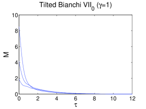
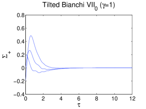
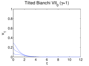
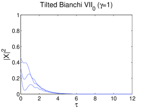
Figure 3. Plots of $M$, $\Sigma_{+}$, $v_{1}$ and $|{\bf X}|^{2}$ for $\gamma=1$, illustrating the rate at which $M$ (and all other variables) tend to zero.

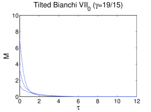
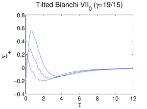
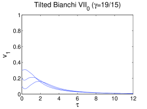
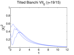
Figure 4. Plots of $M$, $\Sigma_{+}$, $v_{1}$ and $|{\bf X}|^{2}$ for $\gamma=19/15$, illustrating the rate at which $M$ tends to zero. Compare the slow approach of $\Sigma_{+}$,$v_{1}$ and $|{\bf X}|^{2}$ towards zero with the corresponding plots with $\gamma=1$.

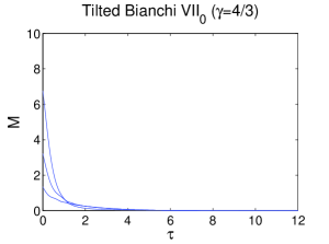
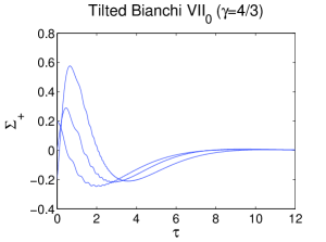
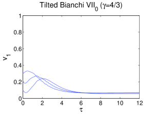
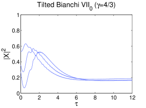
Figure 5. Plots of $M$, $\Sigma_{+}$, $v_{1}$ and $|{\bf X}|^{2}$ for $\gamma=4/3$, illustrating the rate at which $M$ tends to zero. Note how the variables $v_{1}$ and $|{\bf X}|^{2}$ do not approach a unique value.

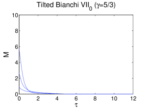
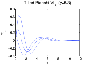
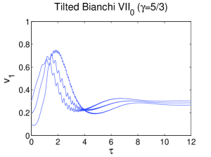
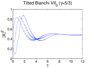
Figure 6. Plots of $M$, $\Sigma_{+}$, $v_{1}$ and $|{\bf X}|^{2}$ for $\gamma=5/3$, illustrating the rate at which $M$ tends to zero. Note how the variables $v_{1}$ and $|{\bf X}|^{2}$ do not approach a unique value. Also notice the oscillatory behavior and how it dampens.

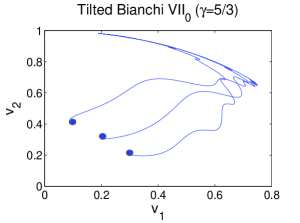
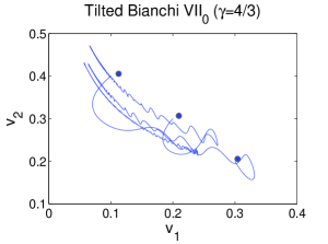
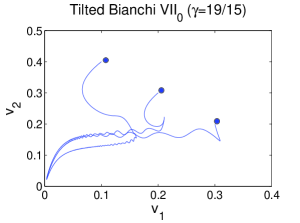
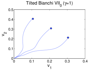
Figure 7. Phase portraits of $v_{1}$ versus $v_{2}$ for different values of $\gamma$ illustrating the fundamental differences in the asymptotic states in each case. Note how $v_{1}^{2}+v_{2}^{2}\to 0$ for $\gamma=1$ and $\gamma=19/15$, $v_{1}^{2}+v_{2}^{2}\to V_{0}^{2}\not=0$ for $\gamma=4/3$ and $v_{1}^{2}+v_{2}^{2}\to 1$ for $\gamma=5/3$.

References

- [1] G.F.R. Ellis and M.A.H. MacCallum, Comm. Math. Phys. 12 (1969) 108
- [2] C.G. Hewitt and J. Wainwright in Dynamical Systems in Cosmology, eds: J. Wainwright and G.F.R. Ellis, Cambridge University Press (1997)
- [3] A.A. Coley, Dynamical Systems and Cosmology, Kluwer, Academic Publishers (2003)
- [4] J.D. Barrow and D.H. Sonoda, Phys. Reports 139 (1986) 1
- [5] K.Rosquist and R.T. Jantzen, Phys. Reports 166 (1988) 89
- [6] O.I. Bogoyavlenskii Methods in the Qualitative Theory of Dynamical Systems in Astrophysics and Gas Dynamics Springer-Verlag (1985).
- [7] A.R. King and G.F.R. Ellis, Commun. Math. Phys. 31 (1973) 209
- [8] D. Hobill, A.B. Burd and A.A. Coley, eds., 1994, Deterministic chaos in general relativity, NATO ASI Series B, vol 332 (Plenum Press, New York).
- [9] H. Ringström, Annales Henri Poincare 2 (2001) 405
- [10] C.G. Hewitt and J. Wainwright, Class. Quant. Grav. 10 (1993) 99
- [11] C.G. Hewitt, R. Bridson, J. Wainwright, Gen. Rel. Grav. 33 (2001) 65
- [12] I.S. Shikin, Sov. Phys. JETP 41 (1976) 794
- [13] C.B. Collins, Comm. Math. Phys. 39 (1974) 131
- [14] C.B. Collins and G. F. R.Ellis, Phys. Rep. 56 (1979) 65
- [15] C.G. Hewitt and J. Wainwright, Phys. Rev. D46 (1992) 4242
- [16] D. Harnett, Tilted Bianchi type V cosmologies with vorticity, Master’s thesis, University of Waterloo, Canada, 1996
- [17] S. Hervik, Class. Quantum Grav. 21 (2004) 2301
- [18] A.A. Coley and S. Hervik, Class. Quantum Grav. 21 (2004) 4193
- [19] A.A. Coley and S. Hervik, Class. Quantum Grav. 22 (2005) 579
- [20] S. Hervik, R.J. van den Hoogen and A.A. Coley, Class. Quantum Grav. 22 (2005) 607
- [21] J. Wainwright, M.J. Hancock and C. Uggla, Class. Quant. Grav. 16 (1999) 2577
- [22] U.S. Nilsson, M.J. Hancock and J. Wainwright, Class. Quant. Grav. 17 (2000) 3119
- [23] B.J. Carr and A.A. Coley, Class. Quant. Grav. 16 (1999) R31
- [24] B.J. Carr and A.A. Coley, gr-qc/0508039
- [25] W.C. Lim, R.J. Deeley and J. Wainwright, in preparation.
- [26] J.D. Barrow and F.J. Tipler, Nature 276 (1978) 453
- [27] J.D. Barrow and S. Hervik, Class. Quantum Grav. 19 (2002) 5173
- [28] J.D. Barrow and S. Hervik, Class. Quantum Grav. 20 (2003) 2841
- [29] P. Apostolopoulos, gr-qc/0407040
- [30] V.A. Belinskii, I.M. Khalatnikov and E.M. Lifshitz, Adv. Phys. 31 (1982) 639
- [31] R.M. Wald, Phys. Rev. D28 (1983) 2118
- [32] A.D. Rendall, Math. Proc. Camb. Phil. Soc. 118 (1995) 511.