UNIVERSITY OF MINNESOTA
This is to certify that I have examined this copy of a doctoral thesis
by
NICOLAE TARFULEA
and have found that is is complete and satisfactory in all respects,and that any and all revisions required by the finalexamining committee have been made.
DR. DOUGLAS N. ARNOLD
Name of Faculty Advisor
Signature of Faculty Advisor
Date
GRADUATE SCHOOL
Constraint Preserving Boundary Conditions forHyperbolic Formulations of Einstein’s Equations
A THESISSUBMITTED TO THE GRADUATE SCHOOLOF THE UNIVERSITY OF MINNESOTABY
Nicolae Tarfulea
IN PARTIAL FULFILLMENT OF THE REQUIREMENTSFOR THE DEGREE OFDOCTOR OF PHILOSOPHY
Dr. Douglas N. Arnold, Advisor
July 2004
©Nicolae Tarfulea 2004
Acknowledgments
I am most grateful and indebted to my thesis advisor, Prof. Douglas N. Arnold, for the large doses of guidance, patience, and encouragement he has shown me during my time at University of Minnesota and Penn State University.
I wish to thank my other thesis committee members Professors Carme Calderer, Bernardo Cockburn, and Fernando Reitich for their support and insightful commentaries on my work.
A substantial part of this thesis was written while I was supported by the University of Minnesota Doctoral Dissertation Fellowship, which is gratefully acknowledged.
Abstract
Einstein’s system of equations in the ADM decomposition involves two subsystems of equations: evolution equations and constraint equations. For numerical relativity, one typically solves the constraint equations only on the initial time slice, and then uses the evolution equations to advance the solution in time. Our interest is in the case when the spatial domain is bounded and appropriate boundary conditions are imposed. A key difficulty, which we address in this thesis, is what boundary conditions to place at the artificial boundary that lead to long time stable numerical solutions. We develop an effective technique for finding well-posed constraint preserving boundary conditions for constrained first order symmetric hyperbolic systems. By using this technique, we study the preservation of constraints by some first order symmetric hyperbolic formulations of Einstein’s equations derived from the ADM decomposition linearized around Minkowski spacetime with arbitrary lapse and shift perturbations, and the closely related question of their equivalence with the linearized ADM system. Our main result is the finding of well-posed maximal nonnegative constraint preserving boundary conditions for each of the first order symmetric hyperbolic formulations under investigation, for which the unique solution of the corresponding initial boundary value problem provides a solution to the linearized ADM system on polyhedral domains.
We indicate how to transform first order symmetric hyperbolic systems with constraints into equivalent unconstrained first order symmetric hyperbolic systems (extended systems) by building-in the constraints. We analyze and prove the equivalence between the original and extended systems in both the case of pure Cauchy problem and initial boundary value problem. These results seem to be very useful for transforming constrained numerical simulations into unconstrained ones. As applications, we derive the extended systems corresponding to the very same hyperbolic formulations of Einstein’s equations for which boundary conditions consistent with the constraints have been found. Boundary conditions for these extended systems that make them equivalent to the original constrained systems are provided.
Chapter 1 Introduction
1.1 Background and Motivations
In a nutshell, general relativity says that “matter tells space how to curve, while the curvature of space tells matter how to move,” in a now famous phrase that the physicist John Wheeler once said. So, general relativity serves both as a theory of space and time and as a theory of gravitation. Einstein began with two basic but subtle and powerful ideas: gravity and acceleration are indistinguishable and matter in free-fall always takes the shortest possible path in curved spacetime. One of Einstein’s most important discoveries was a system of equations which relates spacetime and matter.
While the theory of general relativity has tremendous philosophical implications and has given rise to exotic new physical concepts like black holes and dark matter, it is also crucial in some areas of modern technology such as global positioning systems. All these predictions and applications make general relativity a spectacularly successful theory. However, though a number of its major predictions have been carefully verified by experiments and observations, there are other key predictions, as the existence of gravitational waves, that remain to be fully tested. Einstein’s equations possess solutions describing wavelike undulations in the spacetime. These gravitational waves correspond to ripples in spacetime itself, they are not waves of any substance or medium. Like electromagnetic waves, gravitational waves move at the speed of light and carry energy. In spite of carrying enormous amounts of energy from some of the most violent events in the universe, gravitational waves are almost unobservable. For detecting and analyzing them, state–of–the–art detectors have been built in the United States and overseas. The development of these observatories, just coming online now, is one of the grandest scientific undertakings of our time, and the most expensive project ever funded by the National Science Foundation. With a network of gravitational waves detectors, mankind could open up a whole new window on the cosmic space. The study of the universe using gravitational waves would not be just a simple extension of the optical and electromagnetic possibilities, it would be the exploitation of an entirely new spectrum that could unveil parts and aspects of the universe inaccessible so far.
This enormous technological effort to build ultra-sensitive detectors has been followed by an intense quest for developing computer methods to solve Einstein’s equations. Having invested so much to detect gravitational waves, it is crucial that we be able to interpret the waveforms detected. Most recent investigations in numerical relativity have been based on first order hyperbolic formulations derived from the Arnowitt, Deser, and Misner, or ADM, decomposition [6] (see also [53]) of Einstein’s equations and some results have been obtained in spherical symmetry and axisymmetry. However, in the general three spatial dimensions case, which is needed for the simulation of realistic astrophysical systems, it has not been possible to obtain long term stable and accurate evolutions. One might argue that present day computational resources are still insufficient to carry out high enough resolution three dimensional simulations. However, the difficulty is likely to be more fundamental than that. It seems that there is insufficient understanding of the structure of Einstein’s equations and there are too many unsolved questions related to how to approach them numerically.
Einstein’s system of equations can be decomposed into two subsystems of equations (ADM decomposition): evolution equations and constraint equations (Hamiltonian constraint and momentum constraints). For numerical relativity, one typically solves the constraint equations only on the initial time slice, and then uses the evolution equations to advance the solution in time. A very difficult task is to derive good boundary conditions, and this problem is crucial if one takes into account that it seems impossible to have in the near future the computational power to put the boundaries far away from sources, far enough that they would not affect the region of numerical spacetime being looked at. Traditionally, most numerical relativity treatments have been careful to impose initial data that satisfies the constraints. However, very rarely boundary conditions that lead to well-posedness are used and much less frequently are they consistent with the constraints. Stewart [47] has addressed this subject within Frittelli-Reula formulation [25] linearized around flat space with unit lapse and zero shift in the quarter plane. Both main system and constraints propagate as first order strongly hyperbolic systems. This implies that vanishing values of the constraints at will propagate along characteristics. One wants the values of the incoming constraints at the boundary to vanish. However, one can not just impose them to vanish along the boundaries since the constraints involve derivatives of the fields across the boundary, not just the values of the fields themselves. If the Laplace-Fourier transforms are used, the linearity of the differential equations gives algebraic equations for the transforms of the fields. Stewart deduces boundary conditions for the main system in terms of Laplace-Fourier transforms that preserve the constraints by imposing the incoming modes for the system of constraints to vanish and translating these conditions in terms of Laplace-Fourier transforms of the main system variables. The idea of imposing the vanishing of the incoming constraints as boundary conditions is pursued further in [14] within Einstein-Christoffel formulation [7] in the simple case of spherical symmetry. The radial derivative is eliminated in favor of time derivative in the expression of the incoming constraints by using the main evolution system. In [15], these techniques are refined and employed for the linearized generalized Einstein-Christoffel formulation [36] around flat spacetime with vanishing lapse and shift perturbations on a cubic box. By considering well posed boundary conditions for the constraint system and trading normal derivatives for time and tangential ones, face systems are obtained that need to be solved first together with the compatibility conditions at the edges of the faces. The solutions of the face systems are used to impose well posed constraint preserving boundary conditions for the main system. A construction with several points in common with the one just described can be also found in [49]. These two papers, [15] and [49], are the closest to our work. A different approach can be found in [23], [24], where the authors stray away from the general trend of seeking to impose the constraints along the boundary. Their method consists in making the four components of the Einstein tensor projection along the normal to the boundary vanish. In the case of Einstein-Christoffel formulation restricted to spherical symmetry, the same boundary conditions as in [14] are obtained.
Before we end this brief review, it should also be mentioned here the work done on boundary conditions for Einstein’s equations in harmonic coordinates [48], [49], when Einstein’s equations become a system of second order hyperbolic equations for the metric components. The question of the constraints preservation does not appear here, as it is hidden in the gauge choice (the constraints have to be satisfied only at the initial surface, the harmonic gauge guarantees their preservation in time).
What follows next is a summary of the contents of this dissertation, with emphasis on the ideas that connect the different parts.
1.2 Thesis Organization
This dissertation is divided into three main parts. The first part is represented by Chapter 2 and mainly describes our results concerning first order symmetric hyperbolic (FOSH) systems of partial differential equations. A special attention is being placed on FOSH systems with constraints and their well-posedness with or without boundary conditions. This first part represents a portion of the background theory needed for the rest of the dissertation. The second part, Chapter 3, is focused on the ADM decomposition of Einstein’s equations due to Arnowitt, Deser, and Misner [6] and some important first order hyperbolic formulations derived from it. A novelty in this part is represented by the introduction and analysis in Subsection 3.4.4 of a new first order symmetric hyperbolic formulation of the linearized ADM decomposition due to Arnold [2]. The third part, represented by Chapter 4, is the most important part of this thesis. Here, we address a key difficulty in numerical relativity, the derivation of boundary conditions that lead to well posedness and consistent with the constraints. In the beginning of Chapter 4 we introduce and analyze a simpler model problem which gives good insight for the more complex case of Einstein’s equations. The core of Chapter 4 consists of the analysis of three important first order symmetric hyperbolic formulations of Einstein’s equations for which we provide well-posed constraint-preserving boundary conditions.
In the remainder of this introduction, we will describe the principal results of this dissertation.
1.3 Principal Results
We have developed an effective and general technique for finding well-posed constraint preserving boundary conditions for constrained first order symmetric hyperbolic systems. The key point of this technique is the matching of the general forms of maximal nonnegative boundary conditions for the main system and the system of constraints.
By applying this technique, we study the preservation of constraints by the linearized Einstein-Christoffel system around Minkowski spacetime with arbitrary lapse and shift perturbations, and the closely related question of the equivalence of that system and the linearized ADM system. Our interest is in the case when the spatial domain is bounded and appropriate boundary conditions are imposed. However, we also consider the pure Cauchy problem with the result that the linearized Einstein-Christoffel and ADM systems are equivalent. Our main result is the finding of two distinct sets of well-posed maximal nonnegative constraint preserving boundary conditions for which the unique solution of the corresponding linearized Einstein-Christoffel initial boundary value problem provides a solution to the linearized ADM system on polyhedral domains.
We have also obtained similar results for a very recent symmetric hyperbolic formulation of Einstein’s equations introduced by Alekseenko and Arnold in [3]. A new first order symmetric hyperbolic formulation of linearized Einstein equations due to Arnold [2] is analyzed. Again, the main result is the finding of well-posed constraint preserving boundary conditions. In fact, same ideas should be applicable to some other formulations and/or in different contexts, as, for example, linearization about some other backgrounds. However, while the strategy of finding adequate boundary conditions is similar, the technical apparatus employed depends very much on the formulation under investigation.
Returning to the more general framework of constrained first order symmetric hyperbolic systems, we indicate how to transform such systems into equivalent unconstrained first order symmetric hyperbolic systems (extended systems) by building in the constraints. We also analyze and prove the equivalence between the original and extended systems in both the case of pure Cauchy problem and initial boundary value problem. As applications, we derive extended systems corresponding to the (EC), (AA), and (A) formulations respectively and boundary conditions that make them equivalent to the original constrained systems. These results seem to be useful for transforming constrained numerical simulations into unconstrained ones.
Chapter 2 Symmetric Hyperbolic Systems
2.1 Introduction
In this chapter some basic results on first order symmetric hyperbolic (or FOSH) systems of partial differential equations are briefly reviewed, with special attention being given to systems with constraints and boundary conditions. All these results represent background material relevant to the discussions of the hyperbolic formulations of the Einstein equations which follow in the next chapters. Much more information on hyperbolic systems can be found in the books by John [33], Kreiss and Lorenz [35], Gustafsson, Kreiss and Oliger [27], and Evans [17], among many others.
The second section of this chapter is intended to enlist the basic definition of FOSH systems and some relevant existence and uniqueness results. The third section is dedicated to the analysis of constrained initial value problems in a more abstract framework and in the case of FOSH systems of partial differential equations. The emphasis is on the equivalence between a given system subject to constraints and a corresponding extended unconstrained system. The fourth section deals with boundary conditions for FOSH systems and the connections between the initial boundary value problem for a given FOSH system with constraints and that for the extended system. Section 2.3 and a substantial part of Section 2.4 represent our contribution to the subject.
2.2 Initial Value Problems
In this section we will be concerned with a linear first order system of equations for a column vector with components . Such a system can be written as
| (2.1) |
where . Here are given matrix functions, and is a given -vector field. We will further assume that are of class , with bounded derivatives over , and .
As initial data we prescribe the values of on the hyperplane
| (2.2) |
with . For each , define
| (2.3) |
The system (2.1) is called symmetric hyperbolic if is a symmetric matrix for each , (). Thus, the matrix has only real eigenvalues and the corresponding eigenvectors form a basis of for each , , and .
Remark 1.
More general systems having the form
| (2.4) |
are also called symmetric, provided the matrix functions are symmetric for , and is positive definite. The results set forth below can be easily extended to such systems.
Definition. We say
is a weak solution of the initial value problem (2.1), (2.2) provided
(i) for each and a.e. , and
(ii) .
Here denotes the inner product in .
By using energy methods and the vanishing viscosity technique (see [17], Section 7.3.2.), the following existence and uniqueness result can be proven:
In what follows, we will be more interested in first order symmetric hyperbolic systems with constant coefficients. For such systems, a more general result (including regularity) is valid.
Theorem 2.
The main tool used for proving this theorem is the Fourier transform. The unique solution is given by:
| (2.5) |
2.3 Constrained Initial Value Problems
2.3.1 Abstract Framework
We introduce in this subsection an extended system corresponding to a given constrained system defined on Hilbert spaces and investigate the equivalence of these two systems.
Let us consider the following system subject to constraints:
| (2.6) | |||
| (2.7) | |||
| (2.8) |
where are densely defined closed linear operators on the Hilbert spaces and , and . Moreover, suppose is skew-symmetric and
| (2.9) |
Of course, we assume that the compatibility condition is satisfied. Moreover, another more subtle compatibility condition must hold: . This is because, for any fixed , , for all , and passing to the limit as , it turns out that (since is a closed operator). By operating on (2.6) with , it follows that
where the last equality comes from (2.9).
Remark 2.
If , then the energy of the solution is preserved:
Theorem 3.
Proof.
According to this decomposition of ,
| (2.21) |
where , and .
Since both and are closed and the corresponding projections are continuous,
| (2.22) |
with , and .
2.3.2 Constrained First Order Symmetric Hyperbolic Problems
In this subsection, we will prove a result similar to Theorem 3 for the initial value problem
| (2.28) | |||
| (2.29) | |||
| (2.30) |
where , with constant symmetric matrices, and , with constant matrices. Of course, we assume that (2.9) and the compatibility conditions , , hold.
Theorem 4.
Proof.
Now, let us prove the converse. Denote by
From (2.5), we know that the solution of (2.39)–(2.40) has the following expression
| (2.41) |
The next step in the proof is to show that
| (2.42) |
for all positive integer .
We are going to prove (2.42) by induction.
For , we have
But, since , it follows that by taking the Fourier transform. So
Assume that (2.42) is true for and let us prove it for .
Since , from (2.9), we can see that
| (2.43) |
Applying the Fourier transform to (2.43), we get
Thus,
and the proof of (2.42) is complete.
From (2.42), observe that
| (2.44) |
Same arguments show that
| (2.45) |
2.4 Boundary Conditions
In general, one has to be careful when choosing boundary conditions for a hyperbolic equation (or system). This can be seen even in the simple case of a first order equation in one space dimension (the transport equation). It seems that any acceptable boundary conditions should give the incoming modes into the spatial domain, but they must not try to change the behavior of the outgoing modes. In several dimensions the situation is much more complicated since there is not easy to identify the incoming and outgoing modes. Worse, there may also be waves moving tangent to the boundary, and it is not very clear how these modes could be casted into the boundary conditions.
A few approaches to these questions have been proposed. Some answers have been given by Friedrichs [18] via the “energy method” (see also the work done by Courant and Hilbert). This method provides criteria which are sufficient for constructing boundary conditions that lead to a well-posed problem. Other sufficient conditions have been pointed out by Lax and Phillips in their very interesting work [37]. A necessary and sufficient condition for having a well-posed initial boundary condition has been proved by Hersh [29], but his result was only for systems with constant coefficients and defined on a half-space with non-characteristic boundary conditions. Using Fourier and Laplace transforms, he constructed solutions and derived a necessary and sufficient condition for well-posedness. Later on (in the 1970s and 1980s), more technical approaches came up. Kreiss [34], Majda and Osher [39], among others, proved pretty complicated algebraic results concerning boundary conditions. Remarkably, Kreiss [34] gave a criteria that determine whether a boundary condition is admissible or not. The main point of his approach was the possibility to solve for incoming modes in terms of outgoing modes and boundary conditions. Majda and Osher [39] generalized Kreiss’ theory to the case of uniformly characteristic boundary. Other significant contributions to this subject have been made by Rauch [40], Higdon [30], Secchi [42]–[46], among many others.
2.4.1 Maximal Non-Negative Boundary Conditions
In this subsection we prove a well-posedness result for first order symmetric hyperbolic initial boundary value problems that closely follows the ideas of [37], [40], and [18]. Moreover, we give an algebraic characterization of maximal non-negative boundary conditions which will be used later for determining constraint preserving boundary conditions for some constrained first order symmetric hyperbolic systems.
Consider the symmetric hyperbolic system of equations (2.1) on , where is a bounded domain with a smooth boundary , and .
Set be the outer normal to at , and denote by the boundary matrix
| (2.46) |
We supplement (2.1) with the initial condition (2.2), with , and with linear boundary conditions of the following form
| (2.47) |
Of course, we suppose that the compatibility condition holds on .
In fact, by choosing a function of satisfying (2.2) and (2.47), and changing the variable, we may assume that ; hereafter, we stick with this choice of .
Also, the boundary condition (2.47) may be regarded as
| (2.48) |
Denote the formal adjoint of by
Associated to (2.1), (2.2), and (2.47) (or (2.48)), we consider the adjoint problem
| (2.49) | |||
| (2.50) | |||
| (2.51) |
Next, define the admissible spaces of solutions for both the original problem and the adjoint problem:
and
Observe that, if and , then from Green’s formula
it follows that
Definition. The function is said to be a strong solution of (2.1), (2.2), and (2.47), if the pair belongs to the closure of the graph of ; in other words, if is the limit in the norm of a sequence of functions such that in the norm.
Remark 3.
Definition. The boundary condition (2.47) (or (2.48)) is called non-negative if the matrix is non-negative over
| (2.52) |
Theorem 5.
In order to prove this theorem, we need a couple of intermediate results.
Lemma 6.
For all satisfying the condition (2.52), there exists a positive constant that does not depend on such that
| (2.53) |
Proof.
Symmetric operators with smooth satisfy the following identity
| (2.54) |
where
| (2.55) |
If we integrate (2.54) over , we get
| (2.56) |
Denote by
Then (2.57) recasts into
| (2.58) |
Applying the Gronwall’s lemma to (2.58), it follows that
Hence,
A simple consequence of this lemma is stated next.
Corollary 7.
Lemma 8.
Proof.
According to the expression of , the boundary matrix for is equal to . Hence it suffices to show that is non-positive for each satisfying the adjoint boundary condition.
Arguing by contradiction, suppose that there is a such that .
Consider the linear space . The elements in this space have the form , where and is a real number.
Observe that
which is in contradiction with the maximality of . ∎
Proof.
(of Theorem 5) Existence. We claim that is dense in . Arguing by contradiction, let us suppose the contrary. Then there exists a non-trivial function orthogonal to , i.e.
Therefore, is a weak solution to the adjoint problem corresponding to .
Now, let us prove that . From [37], Theorem 1.1, we get that is a strong solution; therefore there exists a sequence in , such that in and satisfies the (non-negative) adjoint boundary conditions, which implies
So, . In conclusion, if is any element of , then we can find a sequence so that
From Lemma 6, it follows that is a Cauchy sequence in . Thus, there is such that
Uniqueness and Continuous Dependence. Follow from Lemma 6. ∎
There are results concerning the regularity of the solution of (2.1), (2.2), and (2.47). If and then the solution belongs to (see [40]). In fact, this regularity result can be improved by imposing more regularity for and and, in addition, compatibility conditions at the corner . These compatibility conditions are computed in the following fashion. Denote by the orthogonal projection onto . The compatibility condition of order comes from expressing at in terms of and and requiring that the resulting expression vanishes. For example, for , we find on , or for all . For , we have to impose: and on .
Definition. ([40]) A smooth vector field on is called tangential if and only if, for every , . For a positive integer, the space consists of those with the property that for any and tangential fields , (see [8] for more on spaces).
Theorem 9.
We close this subsection by giving an algebraic characterization of maximal non-negative boundary conditions.
Suppose that the boundary matrix has 0–eigenvalues , ,, negative eigenvalues , ,, and positive eigenvalues , , . Let ,, , ,, , ,, be the corresponding eigenvectors. Naturally, at , any vector of has the form . The non-negative condition (2.52) implies:
or
| (2.59) |
Observe that the dimension of must be equal to the number of positive and null eigenvalues counted with their multiplicities.
Now, any can be written as , where , and .
Since is a subspace of codimension , there exists a matrix such that
So, , or
| (2.60) |
where ,,, ,,, ,,, and , with ,,, ,, , and ,,.
Since is maximal non-negative, it follows that , and so,
Therefore, (2.60) reads
| (2.61) |
Observe that the matrix is invertible. If not, there exists so that , and so,
belongs to . But this is in contradiction with (2.59). Hence, is invertible.
So, (2.61) recasts into
Now, we must have (2.59) satisfied, which leads to
Let us state what we have just proved into the following proposition.
Proposition 10.
The boundary condition (2.47) is maximal non-negative if and only if there exists a matrix such that
| (2.62) |
with
The following corollary is an immediate consequence of Proposition 10.
2.4.2 Boundary Conditions for Constrained Systems
In this subsection we establish some connections between the problems (2.28)–(2.30) and (2.39)–(2.40) restricted to a bounded smooth domain . More precisely, we analyze the links between the boundary subspaces and boundary matrices associated to the two problems.
First of all, it is easy to see that the boundary matrix associated to (2.39)–(2.40) is given by
where, as in Subsection 2.4.1, , and , with the outer normal to at .
Lemma 12.
for all .
Proof.
Let and such that . Applying the Fourier transform to (2.9), it follows that , or . So, , for all . ∎
Lemma 13.
| (2.63) |
for all .
Proof.
Clearly,
| (2.64) |
for all .
Lemma 14.
If is a non-negative vector for and , then is non-negative for .
Proof.
Under the given hypotheses, the conclusion is a simple consequence of the following equalities
∎
An immediate corollary of this lemma is
Corollary 15.
The subspace is non-negative for if and only if is non-negative for .
Inhomogeneous Boundary Conditions
In this part, we consider the problem of finding , , , for (2.28), subject to initial condition (2.30), constraints (2.29), and linear inhomogeneous boundary conditions
| (2.68) |
Assume is a vector function defined on for all time such that there exists satisfying the constraint equation (2.29) and on the boundary for all time . Then, by substituting , we arrive to the constrained initial homogeneous boundary value problem
| (2.69) | |||
| (2.70) | |||
| (2.71) | |||
| (2.72) |
It is easy to see that the compatibility conditions for this last problem are satisfied and, in fact, (2.69)–(2.72) is equivalent to the original constrained initial inhomogeneous boundary value problem (2.28)–(2.30) and (2.68). Therefore, in this way and for a restricted set of boundary inhomogeneities, the treatment of inhomogeneous boundary conditions reduces to the treatment of the corresponding homogeneous ones.
Chapter 3 Hyperbolic Formulations of Einstein Equations
3.1 Introduction
Einstein’s equations can be viewed as equations for geometries, that is, its solutions are equivalent classes under spacetime diffeomorphisms of metric tensors. To break this diffeomorphism invariance, Einstein’s equations must be first transformed into a system having a well-posed Cauchy problem. The initial method to solve this problem has been by “fixing the gauge” [26], [12], or in other words, by imposing some conditions on the metric components which would select only one representative from each equivalent class of Einstein’s solutions. By using an ingenious choice of gauge fixing, the so called “harmonic gauge,” Einstein’s equations can be converted to a set of coupled wave equations, one for each metric component. Thus, by prescribing at an initial hypersurface values for the variables and their normal derivatives, one gets unique solutions to this system of wave equations. In Appendix B, we explain this approach, restricted to the linearized case for the sake of simplicity. For a more detailed discussion on this topic, see [41], [19], and references therein.
Another way to deal with the gauge freedom of Einstein’s equations is by prescribing the time foliation along evolution, that is, by prescribing a lapse-shift pair along evolution [6]. Einstein’s equations are then decomposed into evolution equations and constraint equations on the foliation hypersurfaces. An analogous decomposition occurs for Maxwell’s equations, which are canonically split into constraint (divergence) equations and evolution (curl) equations. Both the constraints and the evolution equations are not uniquely determined by this procedure: by taking combinations of the constraints or/and by adding any combination of constraints to any of the evolution equations one gets an equivalent decomposition.
There have been numerical schemes to solve Einstein’s equations based on the ADM decomposition [6], but they have had only a very limited success. The instabilities observed in the ADM based schemes might be at least in part caused by the weakly hyperbolicity of the first order differential reduction of the ADM evolution equations, as argued in [36]. In fact, it is known that some of the stability problems of numerical schemes are due to properties of the equations themselves. By rewriting the equations in a different form, one can obtain better stability of computations for the very same numerical methods.
There have been a large number of first order hyperbolic formulations derived from the ADM decomposition in recent years [4], [5], [25], [7], [9], [10], [36], [3], among others. To give a survey of all of them appears to be a very difficult and extensive task, which is out of the scope of this dissertation (see [28] for a more comprehensive review). All such formulations must be equivalent since they describe the same physical phenomenon. However, they can admit different kinds of unphysical solutions which can grow rapidly in time and overwhelm the physical solution in numerical computations. This is one reason (signaled in [36]) why some formulations of Einstein’s equations behave numerically better than others. From this point of view, first order symmetric hyperbolic formulations of Einstein’s equations present a special attraction for a couple of reasons. First of all, there is a large body of experience and numerical codes that are stable for numerical simulations of FOSH systems derived from various applications (transport equations, wave equations, electromagnetism, etc.). Also, the symmetric hyperbolicity of the system ensures well–posedness and gives bounds on the solution growth. In fact, hyperbolicity refers to algebraic conditions on the principal part of the equations which imply well–posedness, that is, if appropriate initial data is given on an appropriate hypersurface, then a unique solution can be found in a neighborhood of that hypersurface, and that solution depends continuously, with respect to an appropriate norm, on the initial data.
In this chapter, we discuss some FOSH formulations of Einstein’s equations introduced in recent years. Moreover, a new formulation due to Arnold [2] is presented and analyzed.
3.2 Einstein Equations
In general relativity, spacetime is a 4-dimensional manifold of events endowed with a pseudo-Riemannian metric
| (3.1) |
This metric determines curvature on the manifold, and Einstein’s equations relate the curvature at a point of spacetime to the mass-energy there:
| (3.2) |
where is the Einstein tensor and is the energy-momentum tensor.
The Einstein tensor is a second order tensor built from the given metric as follows:
Here is the Ricci tensor:
where
is the Riemann curvature tensor.
The Christoffel symbols are defined as
By we denote the scalar curvature
The energy-momentum tensor can be better understood by looking at two of the simplest energy-momentum tensors in general relativity, namely, the energy-momentum tensors for incoherent matter or dust and for a perfect fluid.
a) Incoherent matter (non-interacting incoherent matter or dust)
Such a field may be characterized by two quantities, the 4-velocity vector field of flow
where is the proper time along the world-line of a dust particle and a scalar field
describing the proper density of the flow, that is, the density which would be measured by an observer moving with the flow (a co-moving observer).
The simplest second-rank tensor we can construct from these two quantities is
and this turn out to be the energy-momentum tensor for the matter field.
Now, let us investigate this tensor in special relativity in Minkowski coordinates. In this case
where and is the proper time defined by
Then, the component of is
This quantity has a simple physical interpretation. First of all, in special relativity, the mass of a body in motion is greater than its rest mass by a factor (). In addition, if we consider a moving three-dimensional volume element, then its volume decreases by a factor through the Lorentz contraction. Thus, from the point of view of a fixed as opposed to a comoving observer, the density increases by a factor . Hence, if a field of material of proper density flows past a fixed observer with velocity , then the observer will measure a density .
The component may therefore be interpreted as the relativistic energy density of the matter field since the only contribution to the energy of the field is from the motion of the matter.
The components of are
Next, we will show that the equations governing the force-free motion of a matter field of dust can be written in the following very succinct way
When , this equation becomes exactly the classical equation of continuity
which expresses the conservation of matter with density moving with velocity . Since matter is the same as energy, it follows that the conservation of energy equation for dust is
Writing the equations corresponding to , we get
Combining this with the equation of continuity, we obtain
which is the Euler equation of motion for a perfect fluid in classical fluid dynamics (in the absence of pressure and external forces).
We have seen that the requirement that the energy-momentum tensor has zero divergence in special relativity is equivalent to demanding conservation of energy and conservation of momentum in the matter field (hence the name energy-momentum tensor).
If we use a non-flat metric, then the conservation law
is replaced by its covariant counterpart
b) Perfect Fluid
A perfect fluid is characterized by three quantities
-
1.
a 4-velocity ,
-
2.
a proper density ,
-
3.
a scalar pressure .
Observe that, if vanishes, a perfect fluid reduces to incoherent matter. This suggests that we take the energy-momentum tensor for a perfect fluid to be of the form
for some symmetric tensor . Since this tensor depends on the velocity and the metric, the simplest assumption we can make is
where and are constants.
Considering the conservation law
in special relativity in Minkowski coordinates and demanding that it reduces in an appropriate limit to the continuity equation and the Euler equation in the absence of body forces, we obtain that and . Therefore, the energy-momentum tensor of a perfect fluid is
In the full theory, we again take the covariant form for the conservation law. In addition, and are related by an equation of state which, in general, is an equation of the form , where is the absolute temperature. Usually, is constant and so, that equation of state reduces to .
The Einstein equations can be viewed in three different ways:
1. The field equations are differential equations for determining the metric tensor from a given energy-momentum tensor . An important case of the equations is when , in which case we are concerned with finding vacuum solutions.
2. The field equations are equations from which the energy-momentum tensor can be read off corresponding to a given metric tensor . In fact, this rarely turns out to be very useful in practice because the resulting are usually physically unrealistic. In particular, it frequently turns out that the energy density goes negative in some region, which is rejected as unphysical.
3. The field equations consist of ten equations connecting twenty quantities (the ten components of and the ten components of ). In this way, the field equations are viewed as constraints on the simultaneous choice of and . This point of view is useful when one can partly specify the geometry and the energy-momentum tensor from physical considerations and then the equations are used to determine both quantities completely.
Remark 4.
-
1.
Each of the 10 equations is a 2nd order PDE in 4 independent variables and 10 unknowns. These 10 equations involve lots of terms.
-
2.
The equations are not independent, due to the Bianchi identities . The energy-momentum tensor also must satisfy these identities.
-
3.
Solutions are not unique, because of gauge freedom (any diffeomorphism of the manifold gives a reparametrization, and hence another solution).
A subtle consequence of Einstein’s equations is that relatively accelerating bodies emit gravitational waves. These gravitational waves are very slight variations in the spacetime metric tensor, which propagate at the speed of light. It is generally believed that extremely violent movements of huge masses, such as collisions of black holes, should generate detectable gravitational waves. However, because of their tiny amplitude, gravitational waves have eluded detection until now. When gravitational waves will be detected, we will must determine the cosmological event that could have caused them. This is in fact an inverse problem and, as usual, we need the solution of the direct problem, which in this case is the numerical solution of Einstein’s equations.
3.3 ADM (3+1) Decomposition
In numerical relativity, the Einstein equations are usually solved as an initial-boundary value problem. In other words, the spacetime is foliated and each slice is characterized by its intrinsic geometry and extrinsic curvature . Subsequent slices are connected via the lapse function and shift vector (see Figure 3.1).

The ADM decomposition [6] (also [53]) of the line element
allows one to express six of the ten components of Einstein’s equations in vacuum as a system of evolution equations for the metric and the extrinsic curvature :
| (3.3) | |||
| (3.4) | |||
| (3.5) | |||
| (3.6) |
where we use a dot to denote time differentiation. The spatial Ricci tensor has components given by second order spatial partial differential operators applied to the spatial metric components . Indices are raised and traces taken with respect to the spatial metric, and parenthesized indices are used to denote the symmetric part of a tensor.
The system of equations for and is first order in time and second order in space. It is not hyperbolic in any usual sense, and direct numerical approaches have been unsuccessful. Therefore, many authors have considered reformulations of (3.3), (3.4) into more standard first order hyperbolic systems. Typically, these approaches involve introducing other variables, like the first spatial derivatives of the spatial metric components (or quantities closely related to them). In the rest of this chapter we present some of the most important first order hyperbolic formulations derived from the ADM decomposition, as well as their linearizations around the Minkowski spacetime. In the last section of this chapter we introduce a new first order symmetric hyperbolic formulation of the linearized ADM equations around Minkowski’s spacetime that has surprising resemblances with Maxwell’s equations. This motivates the introduction of the linearized ADM equations around the flat spacetime in the following subsection.
3.3.1 Linearized ADM Decomposition
In this subsection, we derive the linearized ADM decomposition around the Minkowski spacetime.
A trivial solution to the ADM system (3.3)–(3.6) is the Minkowski spacetime in Cartesian coordinates, given by , , , . To derive the linearization of (3.3)–(3.6) about this solution, we write , , , , where the bars indicate perturbations, assumed to be small. If we substitute these expressions into (3.3)–(3.6) and ignore terms which are at least quadratic in the perturbations and their derivatives, then we obtain a linear system for the perturbations. Dropping the bars, the system is
| (3.7) | |||
| (3.8) | |||
| (3.9) | |||
| (3.10) |
The usual approach to solving the system (3.7)–(3.10) is to begin with initial data and defined on and satisfying the constraint equations (3.9), (3.10), and to define and for via the Cauchy problem for the evolution equations (3.7), (3.8). It can be easily shown that the constraints are then satisfied for all times. Indeed, if we apply the Hamiltonian constraint operator defined in (3.9) to the evolution equation (3.7) and apply the momentum constraint operator defined in (3.10) to the evolution equation (3.8), we obtain the first order symmetric hyperbolic system
Thus if and vanish at , they vanish for all time.
3.4 Hyperbolic Formulations
In this section, we present a number of popular hyperbolic formulations of Einstein’s equations derived from the ADM decomposition. In the last section, we present and analyze a new first order symmetric hyperbolic formulation of Einstein’s equations in the linearized case due to Arnold [2].
3.4.1 Kidder–Scheel–Teukolsky (KST) Family
In this subsection, we present a many-parameter family of hyperbolic representations of Einstein’s equations intoduced by Kidder, Scheel, and Teukolsky [36].
In order to write the evolution equations (3.3) and (3.4) in first-order form, we have to eliminate the second order derivatives of the spatial metric. For this purpose, we introduce new variables
| (3.11) |
Since
the evolution system (3.3), (3.4), together with (3.11) give
| (3.12) | |||
| (3.13) | |||
| (3.14) |
Since we have introduced a new variable that we will evolve independently of the metric, we get additional constraints,
| (3.15) | |||
| (3.16) |
The system (3.12)–(3.14) has been proven to be only weakly hyperbolic. Its characteristic matrix has eigenvalues , but does not have a complete set of eigenvectors. Fortunately, the hyperbolicity of the system can be changed by densitizing the lapse and adding constraints to the evolution equations.
We densitize the lapse by writing: , where , is the densitization parameter, which is an arbitrary constant, and is the lapse density, which will be chosen independent of the dynamical fields.
By adding terms proportional to the constraints, we can modify the evolution system (3.12)–(3.14) without affecting the physical solution:
| (3.17) | |||
| (3.18) |
where represents the same thing that was before, is the Hamiltonian constraint, are the momentum constraints, and are arbitrary parameters.
By carrying out the computations, the evolution system, up to the principal part, is now given by (System 1 in [36]):
| (3.19) |
The eigenvalues of the characteristic matrix of this system are , where
, , and
.
If all are real, then it can be proven that the system is strongly hyperbolic unless one of the following conditions occurs:
| (3.20) | |||
| (3.21) | |||
| (3.22) |
By differentiating the constraints in time, we obtain the following system for the evolution of the constraints (up to the principal part)
| (3.23) |
| (3.24) |
| (3.25) |
| (3.26) |
The eigenvalues for the characteristic matrix of this last system is a subset of the eigenvalues of the evolution equations . Moreover, the constraint evolution system is strongly hyperbolic whenever the regular evolution system is strongly hyperbolic.
We define two new variables: the generalized extrinsic curvature and the generalized derivative of the metric
| (3.27) | |||
| (3.28) |
where we introduce seven additional parameters , and , .
The System 1, (3.19), rewritten for these new variables, up to the principal parts, becomes (System 2 in [36]):
| (3.29) |
where and .
The System 2, (3.29), is also strongly hyperbolic. Moreover, it has the same eigenvalues as System 1, (3.19), but the eigenvectors are different.
Conclusion: By densitizing the lapse, adding constraints to the evolution equations, and changing variables, Kidder, Scheel, and Teukolsky [36] got a twelve-parameter family of strongly hyperbolic formulations of Einstein’s equations. They have observed that the choice of parameters can have a huge impact on the amount of time and accuracy of numerical simulations. Unfortunately, nobody knows why one particular parameter choice behaves much better than others.
Some well-known formulations can be recovered by making appropriate choices for parameters. For example, we can recover the Fritteli–Reula (FR) system [25] if the following choice of parameters is taken in (3.29):
In the next subsection, we present another popular hyperbolic formulation which can be recovered from (3.29).
3.4.2 Einstein–Christoffel (EC) formulation
The EC formulation was originally derived directly from the ADM system (3.3)–(3.6) by Anderson and York [7] in 1999. It can be also recovered if we make the following choice of parameters in (3.29):
In this case, the system is (up to the principal parts):
| (3.30) |
Essentially the coupled part of this system, i.e. the last two equations, is a set of six coupled quasilinear scalar wave equations with nonlinear source terms.
Linearized Einstein–Christoffel Formulation
First, we replace the lapse in (3.3)–(3.6) with where denotes the lapse density. A trivial solution to this system is Minkowski spacetime in Cartesian coordinates, given by , , , . To derive the linearization, we write , , , , where the bars indicate perturbations, assumed to be small. If we substitute these expressions into (3.3)–(3.6) (with ), and ignore terms which are at least quadratic in the perturbations and their derivatives, then we obtain a linear system for the perturbations. Dropping the bars, the system is
| (3.31) | |||
| (3.32) | |||
| (3.33) | |||
| (3.34) |
where we use a dot to denote time differentiation.
Remark 5.
For the linear system the effect of densitizing the lapse is to change the coefficient of the term in (3.32). Had we not densitized, the coefficient would have been instead of , and the derivation of the linearized EC formulation below would not be possible.
The usual approach to solving the system (3.31)–(3.34) is to begin with initial data and defined on and satisfying the constraint equations (3.33), (3.34), and to define and for via the Cauchy problem for the evolution equations (3.31), (3.32). It can be easily shown that the constraints are then satisfied for all times. Indeed, if we apply the Hamiltonian constraint operator defined in (3.33) to the evolution equation (3.31) and apply the momentum constraint operator defined in (3.34) to the evolution equation (3.32), we obtain the first order symmetric hyperbolic system
Thus if and vanish at , they vanish for all time.
The linearized EC formulation provides an alternate approach to obtaining a solution of (3.31)–(3.34) with the given initial data, based on solving a system with better hyperbolicity properties. If , solve (3.31)–(3.34), define
| (3.35) |
Then coincides with the first three terms of the right-hand side of (3.32), so
| (3.36) |
Differentiating (3.35) in time, substituting (3.31), and using the constraint equation (3.34), we obtain
| (3.37) |
where
| (3.38) |
The evolution equations (3.36) and (3.37) for and , together with the evolution equation (3.31) for , form the linearized EC system. As initial data for this system we use the given initial values of and and derive the initial values for from those of based on (3.35):
| (3.39) |
A purpose of this dissertation is to study the preservation of constraints by the linearized EC system and the closely related question of the equivalence of that system and the linearized ADM system. Our interest is in the case when the spatial domain is bounded and appropriate boundary conditions are imposed, but first we consider the result for the pure Cauchy problem in the remainder of this subsection.
Suppose that and satisfy the evolution equations (3.36) and (3.37) (which decouple from (3.31)). If satisfies the momentum constraint (3.34) for all time, then from (3.36) we obtain a constraint which must be satisfied by :
| (3.40) |
The following theorem shows that the pair of constraints (3.34), (3.40) is preserved by the linearized EC evolution.
Theorem 16.
Proof.
It is immediate from the evolution equations that each component satisfies the inhomogeneous wave equation
Applying the momentum constraint operator defined in (3.34), we see that each component satisfies the homogeneous wave equation
| (3.41) |
Now at the initial time by assumption, so if we can show that at the initial time, we can conclude that vanishes for all time. But, from (3.36) and the definition of ,
| (3.42) |
which vanishes at the initial time by assumption. Thus we have shown vanishes for all time, i.e., (3.34) holds. In view of (3.42), (3.40) holds as well. ∎
In view of this theorem it is straightforward to establish the key result that for given initial data satisfying the constraints, the unique solution of the linearized EC evolution equations satisfies the linearized ADM system, and so the linearized ADM system and the linearized EC system are equivalent.
Theorem 17.
Suppose that initial data and are given satisfying the Hamiltonian constraint (3.33) and momentum constraint (3.34), respectively, and that initial data is defined by (3.39). Then the unique solution of the linearized EC evolution equations (3.31), (3.36), (3.37) satisfies the linearized ADM system (3.31)–(3.34).
Proof.
First we show that the initial data defined in (3.35) satisfies the constraint (3.40). Applying the constraint operator in (3.40) to (3.35) we find
which vanishes at time by (3.33). From Theorem 16, we conclude that for all time, i.e., (3.34) holds. Then from (3.31) and (3.34) we see that , and, since vanishes at initial time by assumption, vanishes for all time, i.e., (3.33) holds as well.
3.4.3 Alekseenko–Arnold (AA) Formulation
In this subsection we present a first order symmetric hyperbolic formulation of the full nonlinear ADM system (3.3)–(3.6) which involves fewer unknowns than other hyperbolic formulations and does not require any arbitrary parameters. The hyperbolic systems involves 14 unknowns, namely the components of the extrinsic curvature and eight particular combinations of the first derivatives of the spatial metric. In order to derive the AA formulation, we introduce the notations for the 6-dimensional space of symmetric matrices and for the 8-dimensional space of triply-indexed arrays which are skew-symmetric in the first two indices and satisfy the cyclic property
| (3.43) |
Define the operators , , and by
| (3.44) | |||
| (3.45) | |||
| (3.46) |
respectively. Observe that the operators and are formal adjoints to each other with respect to the scalar products and on the spaces and respectively.
Next, we introduce new variables
| (3.47) |
Observe that belongs to and so, it has eight independent components.
Now we are able to write down the new formulation derived in [3] for the ADM system (3.3)–(3.6).
| (3.48) |
Here is the convective derivative and the omitted terms are algebraic expressions involving , their spatial derivatives , , the lapse , and the shift .
Linearized AA Formulation
The linearized AA formulation provides an alternate approach to obtaining a solution of (3.7)–(3.10) with the given initial data, based on solving a system with better hyperbolicity properties. If and solve (3.7)–(3.10), define
| (3.49) |
where .
Then, proceeding as in [3], we obtain an evolution system for and
| (3.50) | |||
| (3.51) |
where
| (3.52) |
The evolution equations (3.50) and (3.51) for and form the linearized AA system. As initial data for this system we use the given initial values of and and derive the initial values for from those of based on (3.49):
| (3.53) |
As shown in [3], if and satisfy the ADM system and is defined by (3.49), then and satisfy the symmetric hyperbolic system (3.50), (3.51). Conversely, to recover the solution to the ADM system from (3.50), (3.51), the same should be taken at time , and should be given by (3.53). Having determined, the metric perturbation is defined as follows from (3.7)
| (3.54) |
3.4.4 Arnold (A) Formulation
In this subsection, we present and analyze the linearized case of a new first order symmetric hyperbolic formulation of Einstein’s equations due to Arnold [2].
Notations and Identities
We begin by introducing a number of notations and listing a couple of useful identities. Let be a symmetric –matrix function and a vector field (we use underbars for 3-vectors, double underbars for matrices).
is the matrix whose rows are the curls of the rows of
is the matrix whose columns are the curls of the columns of
is the matrix whose rows are the gradients of the entries of
is the vector whose components are the divergences of the rows of .
( being the unit matrix)
For two vector fields and , denote by the following symmetric matrix function .
The proofs of the following identities imply only elementary computations and we leave them to the reader:
| (3.55) |
| (3.56) |
| (3.57) |
| (3.58) |
| (3.59) |
| (3.60) |
| (3.61) |
| (3.62) |
| (3.63) |
| (3.64) |
| (3.65) |
| (3.66) |
| (3.67) |
A New FOSH Formulation of Linearized ADM
If we choose lapse , shift , and linearize the ADM system about the Minkowski’s flat space, the perturbations , of the metric and the extrinsic curvature, respectively, are symmetric matrix fields satisfying
| (3.100) | |||
| (3.141) | |||
| (3.158) | |||
| (3.175) |
Of course, (3.100)–(3.175) is exactly the linearized ADM system (3.7)–(3.10) written in vector–matrix notation.
This system should be supplemented with initial conditions
| (3.176) |
(that satisfy the constraints (3.158) and (3.175)) and boundary conditions if the domain has frontier.
Lemma 18.
| (3.177) |
Theorem 19.
Proof.
Denote by . Then , and . Therefore,
Introduce , and . Then the equations (3.236), (3.235) induce the following first order symmetric hyperbolic system with constraints
| (3.277) | |||
| (3.302) | |||
| (3.319) | |||
| (3.336) |
Here, the initial data is
| (3.337) |
If and satisfy the Hamiltonian constraint (3.158) and the momentum constraint (3.175) respectively, then it is not hard to see that the compatibility conditions and are satisfied.
Proposition 20.
Proof.
From construction, it is obvious that once we have a solution for (3.100)–(3.176), then (3.277)–(3.337) has solution.
Let us prove that the converse is also valid. Assume we can solve (3.277)–(3.337) and define
| (3.362) | |||
| (3.395) |
Obviously, and and so, (3.176) is verified. Now, we prove that (3.158) is satisfied. From (3.61) it follows that
| (3.396) |
and from here
| (3.397) |
Since , we get for all time.
Next, we show that satisfies (3.175). From (3.302), (3.337), and (3.362) it follows that
| (3.398) |
for all time. By using (3.277)–(3.302), (3.362), and (3.398) we can see that satisfies the initial value problem
| (3.439) | |||
| (3.472) |
whose only solution is the trivial solution. So, for all time.
Equivalent Unconstrained Initial Value Problem
Therefore, we can transform our system into a symmetric hyperbolic (unconstrained) system
| (3.474) |
The initial data for the above system reads
| (3.475) |
Chapter 4 Boundary Conditions for Einstein’s Equations
4.1 Introduction
A very difficult situation is encountered if initial boundary value problems are considered for Einstein’s equations. It has become clear in the numerical relativity community that in order for constraints to be preserved during evolution, the boundary conditions have to be chosen in an appropriate way. This problem is widely open in its full generality for Einstein’s equations. The main difficulty comes from the necessity to deal with unphysical instabilities, which will always be triggered in numerical simulations by round-off errors and lead to constraint violating numerical solutions. In other words, the numerical solution of the initial boundary value problem with constrained initial data fails to solve the constraints soon after the initial time. This serious drawback motivates the quest for boundary conditions that preserve the constraints. Only in the last few years work along this line has been pursued; see [47], [14], [15], [23], [24], [31], among others. In view of our work, of particular interest is the recent paper by Calabrese et al. [15] on the generalized [36] Einstein–Christoffel formulation [7] linearized around Minkowski spacetime, which employs techniques with some points in common with the ones used in our approach of the problem in this chapter. It is here where the differential equations satisfied by the constraints are very important. In particular, if they form a hyperbolic system, then the study of its well–posedness is proven to be a very good starting point for what boundary conditions we must force upon the evolution system for the dynamical variables. By exploiting this idea, we have been able to develop a technique that provides maximal nonnegative constraint preserving boundary conditions for various hyperbolic formulations of Einstein’s equations in the linearized case. This entire chapter represents our original contribution to the subject.
4.2 Model Problem
In this section we consider a constrained first order symmetric hyperbolic system, which, as we shall prove, admits well-posed constraint preserving boundary conditions. The analysis of this model problem gives a good deal of insight for finding same type of boundary conditions for various hyperbolic formulations of Einstein’s equations. Although the problem is simple, the techniques used here reveal our basic strategy to tackle the more complex case of Einstein’s equations.
For and in , we are interested in finding a solution for the following first order symmetric hyperbolic system
| (4.1) |
with the initial data
| (4.2) |
and subject to the constraint
| (4.3) |
Assume that the initial conditions (4.2) are compatible with the constraint (4.3)
| (4.4) |
Also, assume that the forcing terms satisfy the compatibility condition
| (4.5) |
Then, for the pure Cauchy problem (4.1), (4.2), it can be easily shown that the constraint (4.3) is satisfied for all time. Indeed, if we differentiate twice in time the constraint (4.3) and use the main system (4.1), it follows that
| (4.6) |
Since for all time, it follows that satisfies the wave equation on .
| (4.7) |
Moreover, from the compatibility conditions (4.4)
| (4.8) |
So,
| (4.9) |
Also,
| (4.10) |
The first term on the right side vanishes from the second compatibility condition in (4.4). The second term vanishes because of (4.5). Thus,
| (4.11) |
From (4.7), (4.9), and (4.11), we conclude that for all time.
4.2.1 Constraint-Preserving Boundary Conditions for the Model Problem
In this subsection, we are interested in finding suitable boundary conditions for (4.1) on the boundary of a bounded spatial domain such that the solution of the resulting initial-boundary value problem satisfies the constraint (4.3) for all time.
On Polyhedral Domains
First, we investigate the existence of constraint-preserving boundary conditions on polyhedral domains, with the result that there exists a set of such boundary conditions. Moreover, these boundary conditions are also maximal nonnegative, and so, the corresponding initial-boundary value problem is well-posed.

Let be a polyhedral domain in . Consider an arbitrary face of and let denote its exterior unit normal. Denote by and two additional vectors which together form an orthonormal basis (see Figure 4.1). The projection operator orthogonal to is then given by (and does not depend on the particular choice of these tangential vectors). Note that
| (4.12) |
Consequently,
| (4.13) |
We shall prove that the following set of boundary conditions
| (4.14) |
is constraint-preserving and, together with (4.1) and (4.2), leads to a well-posed initial-boundary value problem. Observe that these boundary conditions can be written as well:
| (4.15) |
Therefore, they do not depend on the particular choice of the tangential vectors and .
Theorem 21.
Proof.
First we prove that on any boundary face of . From the first identity of (4.12), the constraint can be decomposed as follows
| (4.16) |
By the third equation in (4.1) and the second identity of (4.12), (4.16) reads
| (4.17) |
From the boundary conditions (4.15), we know that for all time, and so the first term on the right-hand side vanishes. Similarly, we know that on the boundary face, and so the second term vanishes as well (since the differential operator is purely tangential). We have established that holds on any boundary face of .
Theorem 22.
The differential system (4.1), together with initial data (4.2) and boundary conditions (4.15) is well-posed. Furthermore, if the initial conditions , , and the forcing terms are given satisfying the compatibility conditions (4.4) and (4.5) respectively, then the solution satisfies the constraint (4.3) for all time.
Proof.
We begin by showing that the boundary conditions (4.15) are maximal nonnegative for the hyperbolic system (4.1), and so, according to the classical theory of [18] and [37] (see also [40]), the initial-boundary value problem is well-posed. We recall the definition of maximal nonnegative boundary conditions. Let . Obviously, . The boundary operator associated to the hyperbolic system (4.1) is the symmetric linear operator which assigns to any element of the element defined by
| (4.18) |
A subspace of is called nonnegative for if
| (4.19) |
whenever and defined by (4.18). We claim that the subspace defined by the boundary conditions (4.15) is maximal nonnegative. The dimension of is clearly 12. Since has three positive, nine zero, and three negative eigenvalues, a nonnegative subspace is maximal nonnegative if and only if it has dimension 12, and so, the proof reduces to the verification of nonnegativity condition (4.19). Since
| (4.20) |
the verification of (4.19) reduces to showing that whenever (4.15) holds. In fact, we prove that if the boundary conditions (4.15) are verified. For this, we use the orthogonal decomposition of . From the second boundary condition in (4.15), the tangential part of vanishes. Thus, . From the first boundary condition in (4.15), the right-hand side vanishes, and so, . This ends the proof of the maximal nonnegativity of the boundary conditions (4.15).
The fact that the solution satisfies the constraint for all time follows from Theorem 21. ∎
On Piecewise Regular Domains
Here we investigate the existence of constraint-preserving boundary conditions on more general domains, namely on piecewise regular domains. We shall provide a set of such boundary conditions which generalize the boundary conditions (4.15). Although these boundary conditions are not maximal nonnegative in general, and so, the classical theory of [18] and [37] can not be employed, we have been able to prove an energy inequality which is a key ingredient in proving well-posedness.
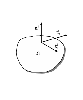
Let be a bounded domain in . Assume that the boundary of , denoted by is an almost everywhere regular surface in , that is, for almost every point , there exists an open set in and a difeomorphism , , of an open set onto . The mapping is called a parameterization or a system of (local) coordinates in a neighborhood of . From [38], Corollary 2, p. 183, we know that for all there exists a parameterization in a neighborhood of such that the coordinate curves intersect orthogonally for each (such a is called orthogonal parameterization). Since working in an orthogonal parameterization turns out to simplify our computations, we assume that is an orthogonal parameterization. At each point of define the tangent vectors , , and the unit normal to the boundary (see Figure 4.2)
| (4.21) |
For the given parameterization , the derivatives of belong to the tangential plane and are given by
| (4.22) |
The trace of the matrix does not depend on the choice of parameterization. Hence, the mean curvature , which is one half of the trace of , is parameterization independent. Since the principal curvatures and are the roots of the quadratic equation
we can write
| (4.23) |
We shall prove that the following set of boundary conditions
| (4.24) |
is constraint-preserving and, together with (4.1) and (4.2), leads to well-posedness.
First we prove the equivalent of Theorem 21 under the new circumstances.
Theorem 23.
Proof.
Let , , and be the coefficients of the first fundamental form in the basis . The derivatives of the vectors and in the basis are (see [38], p. 232):
| (4.25) |
where are the Christoffel symbols and , , and .
Since the constraint satisfies the wave equation (4.7) with zero initial conditions (4.9), (4.11), the proof of this theorem reduces to prove that on the boundary for all time. From the first identity of (4.12), observe that on the boundary the constraint is . From the main system (4.1), the first term of the right-hand side is equal to . Since the parameterization is orthogonal, the tangential projection of is
where , , represent the components of the tangent vector , . By the Leibnitz rule of differentiation, the right-hand side of this identity can be written as follows
| (4.26) |
The first two terms of the right-hand side vanish due to the second boundary condition in (4.24) combined with the tangentiality of the differential operators , . Furthermore, by the chain rule, , . Thus,
| (4.27) |
By the first identity in (4.25), the first term of the right-hand side of (4.27) is
| (4.28) |
The first two terms of the right side of the last identity vanish due to the second boundary condition in (4.24), and so
| (4.29) |
Similarly,
| (4.30) |
Thus,
| (4.31) |
Therefore, . By the first equation in (4.1), , combined with the definition of the mean curvature, , it follows that . Finally, from the first boundary condition in (4.24), on for all time. This ends the proof of this theorem. ∎
Theorem 24.
Let be a bounded domain in with (a.e.) regular boundary and the mean curvature almost everywhere. Given the initial conditions , , and the forcing terms satisfying the compatibility conditions (4.4) and (4.5) respectively, the system of differential equations (4.1), together with the boundary conditions (4.24) and the initial conditions (4.2), is well-posed. Moreover, its solution satisfies the constraint (4.3) for all time.
Proof.
For any solution , , of (4.1) satisfying the boundary conditions (4.24), define the energy
Differentiating in time, we obtain
By the system (4.1), the derivatives in time can be substituted for spatial derivatives, and so
Integrating by parts, it follows that
By the orthogonal decomposition of , we obtain . In view of the second boundary condition in (4.24), the second term of the right-hand side vanishes. Thus, , and so
Due to the second boundary condition in (4.24), the boundary integral vanishes. Therefore,
Now, since (), it is easy to see that
where for all positive time . By the Gronwall inequality, . This energy estimate is a key ingredient in proving well-posedness by Galerkin approximations.
4.3 Einstein-Christoffel Formulation
4.3.1 Maximal Nonnegative Constraint-Preserving Boundary Conditions
In this section, we provide maximal nonnegative boundary conditions for the linearized EC system which are constraint-preserving in the sense that the analogue of Theorem 16 is true for the initial–boundary value problem. This will then imply the analogue of Theorem 17. We assume that is a polyhedral domain (see Figure 4.1) and use the notations introduced in Subsection 4.2.1.
First we consider the following boundary conditions on the face:
| (4.32) |
These can be written as well:
| (4.33) |
and so do not depend on the choice of basis for the tangent space. We begin by showing that these boundary conditions are maximal nonnegative for the hyperbolic system (3.36), (3.37), and so, according to the classical theory of [18] and [37], the initial–boundary value problem is well-posed.
Let denote the vector space of pairs of constant tensors both symmetric with respect to the indices and . Thus . The boundary operator associated to the evolution equations (3.36), (3.37) is the symmetric linear operator given by
| (4.34) |
A subspace of is nonnegative for if
| (4.35) |
whenever and is defined by (4.34). The subspace is maximal nonnegative if also no larger subspace has this property. The eingenvalues of , together with the corresponding eigenvectors , are the following:
with multiplicity 12 and eingenvectors: , , , , , , , , , , , ,
with multiplicity six and eingenvectors: , , , , , ,
with multiplicity six and eingenvectors: , , , , , .
Since has six positive, 12 zero, and six negative eigenvalues, a nonnegative subspace is maximal nonnegative if and only if it has dimension . Our claim is that the subspace defined by (4.32) is maximal nonnegative. The dimension is clearly . In view of (4.34), the verification of (4.35) reduces to showing that whenever (4.32) holds. In fact, , that is, and are orthogonal (when (4.32) holds). To see this, we use orthogonal expansions of each based on the normal and tangential components:
| (4.36) | ||||
| (4.37) |
In view of the boundary conditions (in the form (4.33)), the two inner terms on the right-hand side of (4.36) and the two outer terms on the right-hand side of (4.37) vanish, and so the orthogonality is evident.
Next we show that the boundary conditions are constraint-preserving. This is based on the following lemma.
Lemma 25.
Proof.
In fact we shall show that (so also ) and , which, by (4.13) implies (4.38). First note that
where we have used the first identity in (4.12). Contracting with gives
where now we have used the equation (3.37) (with ) for the first and last term and the second identity in (4.12) for the middle term. From the boundary conditions we know that , and so the first term on the right-hand side vanishes. Similarly, we know that on the boundary face, and so the second term vanishes as well (since the differential operator is purely tangential). Finally, , and so the third term vanishes. We have established that holds on the face.
To show that on the face, we start with the identity
Similarly
Therefore,
For the last three terms, we again use (3.37) to replace with and argue as before to see that these terms vanish. For the first term we notice that (from (3.36) and (3.37) with vanishing and ). Since vanishes on the boundary, this term vanishes. Finally we recognize that the second term is the tangential Laplacian, applied to the quantity , which vanishes. This concludes the proof of (4.38). ∎
The next theorem asserts that the boundary conditions are constraint-preserving.
Theorem 26.
Proof.
Exactly as for Theorem 16 we find that satisfies the wave equation (3.41) and both and vanish at the initial time. Define the usual energy
Clearly . From (3.41) and integration by parts
| (4.39) |
Therefore, if and , we can invoke Lemma 25, and conclude that is constant in time. Hence vanishes identically. Thus is constant, and, since it vanishes at time , it vanishes for all time. This establishes the theorem under the additional assumption that and vanish.
To extend to the case of general and we use Duhamel’s principle. Let denote the solution operator associated to the homogeneous boundary value problem. That is, given functions , on , define where , is the solution to the homogeneous evolution equations
satisfying the boundary conditions and assuming the given initial values. Then Duhamel’s principle represents the solution , of the inhomogeneous initial-boundary value problem (3.36), (3.37), (4.32) as
| (4.40) |
Now it is easy to check that the momentum constraint (3.34) is satisfied when is replaced by (for any smooth function ), and the constraint (3.40) is satisfied when is replaced by defined by (3.38) (for any smooth function ). Hence the integrand in (4.40) satisfies the constraints by the result for the homogeneous case, as does the first term on the right-hand side, and thus the constraints are indeed satisfied by , . ∎
The analogue of Theorem 17 for the initial–boundary value problem follows from the preceding theorem exactly as before.
Theorem 27.
Let be a polyhedral domain. Suppose that initial data and are given satisfying the Hamiltonian constraint (3.33) and momentum constraint (3.34), respectively, and that initial data is defined by (3.39). Then the unique solution of the linearized EC initial–boundary value problem (3.31), (3.36), (3.37), together with the boundary conditions (4.32) satisfies the linearized ADM system (3.31)–(3.34) in .
We close by noting a second set of boundary conditions which are maximal nonnegative and constraint-preserving. These are
| (4.41) |
or, equivalently,
Now when we make an orthogonal expansion as in (4.36), (4.37), the outer terms on the right-hand side of the first equation and the inner terms on the right-hand side of the second equation vanish (it was the reverse before), so we again have the necessary orthogonality to demonstrate that the boundary conditions are maximal nonnegative. Similarly, to prove the analogue of Lemma 25, for these boundary conditions we show that the tangential component of vanishes and the normal component of vanishes (it was the reverse before). Otherwise the analysis is essentially the same as for the boundary conditions (4.32).
4.3.2 Extended EC System
In this section we indicate an extended initial boundary value problem whose solution solves the linearized ADM system (3.31)–(3.34) in . This approach could present advantages from the numerical point of view since the momentum constraint is “built-in”, and so controlled for all time. The new system consists of (3.31), (3.37), and two new sets of equations corresponding to (3.36)
| (4.42) |
and to a new three dimensional vector field defined by
| (4.43) |
respectively. Observe that the additional terms that appear on the right-hand side of (4.42) compared with (3.36) are nothing but the negative components of the formal adjoint of the momentum constraint operator applied to .
Let be the vector space of quadruples of constant tensors symmetric with respect to the indices and . Thus . The boundary operator in this case is given by
| (4.44) |
The boundary operator associated to the evolution equations (3.31), (4.42), (3.37), and (4.43) has six positive, 21 zero, and six negative eigenvalues. Therefore, a nonnegative subspace is maximal nonnegative if and only if it has dimension 27. We claim that the following boundary conditions are maximal nonnegative for (3.31), (4.42), (3.37), and (4.43)
| (4.45) |
These can be written as well:
| (4.46) |
and so do not depend on the choice of basis for the tangent space.
Let us prove the claim that the subspace defined by (4.45) is maximal nonnegative. Obviously, . Hence, it remains to be proven that is also nonnegative. In view of (4.44), the verification of nonnegativity of reduces to showing that
| (4.47) |
whenever (4.45) holds. In fact, we can prove that the left-hand side of (4.47) vanishes pending (4.45) holds. From the boundary conditions (in the form (4.46)) and the orthogonal expansions (4.36) and (4.37) of and , respectively, the first term on the right-hand side of (4.47) reduces to . Then, combining the first and third terms of the left-hand side of (4.47) gives . Finally, by using the orthogonal decomposition and the first part of the boundary conditions (4.46) the second term of the left-hand side of (4.47) is , which is precisely the negative sum of the first and third terms of the left-hand side of (4.47). This concludes the proof of (4.47).
Theorem 28.
Let be a polyhedral domain. Suppose that the initial data and are given satisfying the Hamiltonian (3.33) and momentum constraints (3.34), respectively, is defined by (3.35), and . Then the unique solution of the initial boundary value problem (3.31), (4.42), (3.37), and (4.43), together with the boundary conditions (4.45), satisfies the properties for all time, and solves the linearized ADM system (3.31)–(3.34) in .
Proof.
Observe that the solution of the initial boundary value problem (3.31), (3.36), (3.37), and (4.32) (boundary conditions), together with for all time, is the unique solution of the initial boundary value problem (3.31), (4.42), (3.37), and (4.43), together with the boundary conditions (4.45). The conclusion follows from Theorem 27. ∎
4.3.3 Inhomogeneous Boundary Conditions
In this subsection we provide well-posed constraint-preserving inhomogeneous boundary conditions for (3.31), (3.36), and (3.37) corresponding to the two sets of boundary conditions (4.32), and (4.41), respectively. The first set of inhomogeneous boundary conditions corresponds to (4.32) and can be written in the following form
| (4.50) |
where , , with and given in for all time and satisfying the constraints (3.34) and (3.40), respectively. The matter of choosing and is deferred to the Appendix A.
Theorem 29.
Proof.
The analogue of Theorem 27 for the case of the inhomogeneous boundary conditions (4.50) follows from the preceding theorem by using the same arguments as in the proof of Theorem 17.
Theorem 30.
Let be a polyhedral domain. Suppose that initial data and are given satisfying the Hamiltonian constraint (3.33) and momentum constraint (3.34), respectively, and that initial data is defined by (3.39). Then the unique solution of the linearized EC initial–boundary value problem (3.31), (3.36), (3.37), together with the inhomogeneous boundary conditions (4.50) satisfies the linearized ADM system (3.31)–(3.34) in .
Note that there is a second set of inhomogeneous boundary conditions corresponding to (4.41) for which Theorem 29 and Theorem 30 remain valid. These are
| (4.51) |
where again , , with and given and satisfying the constraints (3.34) and (3.40), respectively.
Similar considerations can be made for the extended system introduced in the previous section. There are two sets of inhomogeneous boundary conditions for which the extended system produces solutions of the linearized ADM system (3.31)–(3.34) on a polyhedral domain . These are
| (4.52) |
and, respectively,
| (4.53) |
where and are defined as before.
The next theorem is an extension of Theorem 28 to the case of inhomogeneous boundary conditions.
Theorem 31.
Let be a polyhedral domain. Suppose that the initial data and are given satisfying the Hamiltonian (3.33) and momentum constraints (3.34), respectively, is defined by (3.35), and . Then the unique solution of the initial boundary value problem (3.31), (4.42), (3.37), and (4.43), together with the inhomogeneous boundary conditions (4.52) (or (4.53)), satisfies the properties for all time, and solves the linearized ADM system (3.31)–(3.34) in .
Proof.
Note that the solution of the initial boundary value problem (3.31), (3.36), (3.37), and (4.50) (or (4.51), respectively), together with for all time, is the unique solution of the initial boundary value problem (3.31), (4.42), (3.37), and (4.43), together with the boundary conditions (4.52) (or (4.53), respectively). The conclusion follows from Theorem 30. ∎
4.4 Alekseenko-Arnold Formulation
4.4.1 Maximal Nonnegative Constraint-Preserving Boundary Conditions
The equivalence of (3.50), (3.51) and the linearized ADM system has been studied in the second section of [3] for the case of pure initial value problem with the result that for given initial data satisfying the constraints, the unique solution of the linearized AA evolution equations satisfies the linearized ADM system, and so the linearized ADM system and the linearized AA system are equivalent (see [3], Theorem 1.). Our interest is in the case when the spatial domain is bounded and appropriate boundary conditions are imposed. In this subsection, we provide maximal nonnegative boundary conditions for the linearized AA system which are constraint-preserving. This will then imply the analogue of the equivalence result proven in [3] (Theorem 1.) for the case of bounded domains. The ideas and techniques used in this section have many points in common to those used in Section 4.3 for the case of EC formulation.
Assume that is a polyhedral domain. Consider an arbitrary face of and let denote its exterior unit normal. Denote by and two additional vectors which together form an orthonormal basis (see Figure 4.1).
First we consider the following boundary conditions on the face:
| (4.54) |
These are equivalent to:
| (4.55) |
where is the projection operator to , and so do not depend on the choice of basis for the tangent space. We begin by showing that these boundary conditions are maximal nonnegative for the hyperbolic system (3.50), (3.51), and so, according to the classical theory of [18] and [37], the initial boundary value problem is well-posed.
Let denote the vector space of pairs of constant tensors . Here is symmetric with respect to the indices and , and is a third-order constant tensor which is antisymmetric with respect to the first two indices and satisfies the cyclic identity . Thus . The boundary operator associated to the evolution equations (3.36), (3.37) is the symmetric linear operator given by
| (4.56) |
A subspace of is called nonnegative for if
| (4.57) |
whenever and is defined by (4.56). The subspace is maximal nonnegative if also no larger subspace has this property. Since has five positive, four zero, and five negative eigenvalues, a nonnegative subspace is maximal nonnegative if and only if it has dimension nine. Our claim is that the subspace defined by (4.54) is maximal nonnegative. The dimension is clearly nine. In view of (4.56), the verification of (4.57) reduces to showing that whenever (4.32) holds. In fact, , that is, and are orthogonal (when (4.54) holds). To see this, we use orthogonal expansions of each based on the normal and tangential components:
| (4.58) | ||||
| (4.59) |
In view of the boundary conditions (in the form (4.55)), the two inner terms on the right-hand side of (4.58) and the last term of the right-hand side of (4.59) vanish. Also, the first two terms of the right-hand side of (4.59) vanish due to the antisymmetry of with respect to the first two indices. Thus, the orthogonality is evident.
Next we show that the boundary conditions are constraint-preserving. This is based on the following lemma.
Lemma 32.
Proof.
In fact we shall show that (so also ) and , which, by (4.13) implies (4.60). First note that
Contracting with and using the first identity of (4.12) give
where now we have used the equation (3.51) (with ) for the last term. From the boundary conditions we know that , and so the first term on the right-hand side vanishes (since the differential operator is purely tangential). Similarly, on the boundary face, and so the second term vanishes as well. We have established that holds on the face.
To show that on the face, we start with the identity
Similarly
Therefore,
The second term of the right-hand side vanishes since it involves the tangential Laplacian applied to the quantity , which vanishes. For the third and last terms, we again use (3.51) to replace with and argue as before to see that the resulting terms vanish. For the first term we notice that (from (3.50) and (3.51) with vanishing and ). So, . From and on the face, this identity reduces to .
Finally, . Again, from on the face and the tangentiality of , the first term vanishes. Also, from the boundary conditions and the tangentiality of , the last term vanishes. So, .
From above, , which implies on the face. This concludes the proof of (4.60). ∎
The next theorem asserts that the boundary conditions are constraint-preserving.
Theorem 33.
Proof.
Exactly as in the proof of Theorem 1. of [3], we find that satisfies satisfies the elastic wave equation
| (4.61) |
and both and vanish at the initial time. Define the usual energy
Clearly . From (4.61) and integration by parts
| (4.62) |
Therefore, if and , we can invoke Lemma 32, and conclude that is constant in time. Hence vanishes identically. Thus is constant, and, since it vanishes at time , it vanishes for all time. This establishes the theorem under the additional assumption that and vanish.
To extend to the case of general and we use Duhamel’s principle. Let denote the solution operator associated to the homogeneous boundary value problem. That is, given functions , on , define where , is the solution to the homogeneous evolution equations
satisfying the boundary conditions and assuming the given initial values. Then Duhamel’s principle represents the solution , of the inhomogeneous initial boundary value problem (3.50), (3.51), (4.54) as
| (4.63) |
Now it is easy to check that the momentum constraint (3.10) is satisfied when is replaced by (for any smooth function ), and, from (3.50), for any smooth shift vector . Hence the integrand in (4.63) satisfies the constraints by the result for the homogeneous case, as does the first term on the right-hand side, and thus the constraints are indeed satisfied by , . ∎
The analogue of Theorem 1. of [3] for the initial boundary value problem follows from the preceding theorem exactly as there.
Theorem 34.
Let be a polyhedral domain. Suppose that initial data and are given satisfying the Hamiltonian constraint (3.9) and momentum constraint (3.10), respectively, and that initial data is defined by (3.53). Then the unique solution of the linearized AA initial boundary value problem (3.50), (3.51), and defined by (3.54) together with the boundary conditions (4.54) satisfies the linearized ADM system (3.7)–(3.10) in .
We close by noting a second set of boundary conditions which are maximal nonnegative and constraint-preserving. These are
| (4.64) |
Now when we make an orthogonal expansion as in (4.58), (4.59), the first term on the right-hand side of the first equation and the first two terms on the right-hand side of the second equation vanish. The necessary orthogonality to demonstrate that the boundary conditions are maximal nonnegative follows from the boundary conditions and the antisymmetry of with respect to its first two indices. Similarly, to prove the analogue of Lemma 32 for these boundary conditions, we show that the tangential component of vanishes and the normal component of vanishes (it was the reverse before). The analysis is essentially the same as for the boundary conditions (4.54). However, we need to do some more work here since the vanishing of both tangential component of and normal component of is not enough for proving (4.60). We prove that vanishes on the face. From (3.51), observe that . So, from (3.50) and the antisymmetry of in and , . From (4.64), it follows that the divergence of vanishes on the face. Otherwise the approach follows exactly the ideas and techniques used for the boundary conditions (4.54).
4.4.2 Extended AA System
By using similar ideas and techniques as in Subsection 4.3.2, we indicate an extended initial boundary value problem corresponding to the AA formulation whose solution solves the linearized ADM system (3.7)–(3.10) in . The new system consists of (3.7) for , (3.51), and two new sets of equations, one replacing (3.50)
| (4.65) |
and the other one corresponding to a new three dimensional vector field defined by
| (4.66) |
Observe that the additional terms that appear on the right-hand side of (4.65) compared with (3.50) are precisely the negative components of the formal adjoint of the momentum constraint operator (3.10) applied to .
Let be the vector space of quadruples of constant tensors , where , are symmetric with respect to the indices and and belong to the 8-dimensional space defined in Subsection 3.4.3. Thus . The boundary operator in this case is given by
| (4.67) |
The boundary operator associated to the evolution equations (3.7), (4.65), (3.51), and (4.66) has five positive, 13 zero, and five negative eigenvalues. Therefore, a nonnegative subspace is maximal nonnegative if and only if it has dimension 18. We claim that the following boundary conditions are maximal nonnegative for (3.7), (4.65), (3.51), and (4.66)
| (4.68) |
These can be written as well:
| (4.69) |
and so do not depend on the choice of basis for the tangent space.
Let us prove the claim that the subspace defined by (4.68) is maximal nonnegative. Obviously, . Hence, it remains to be proven that is also nonnegative. In view of (4.67), the verification of nonnegativity of reduces to showing that
| (4.70) |
whenever (4.68) holds. In fact, we can prove that the left-hand side of (4.70) vanishes pending that (4.68) holds:
| (4.71) |
This concludes the proof of (4.70).
Theorem 35.
Let be a polyhedral domain. Suppose that the initial data and are given satisfying the Hamiltonian (3.9) and momentum constraints (3.10), respectively, is defined by (3.53), and . Then the unique solution of the initial boundary value problem (3.7), (4.65), (3.51), and (4.66), together with the boundary conditions (4.68), satisfies the properties for all time, and solves the linearized ADM system (3.7)–(3.10) in .
Proof.
Observe that the solution of the initial boundary value problem (3.7), (3.50), (3.51), and (4.54) (boundary conditions), together with for all time, is the unique solution of the initial boundary value problem (3.7), (4.65), (3.51), and (4.66), together with the boundary conditions (4.68). The conclusion follows from Theorem 34. ∎
4.5 Arnold Formulation
Throughout this section, we will use the notations and results introduced in Subsection 3.4.4. In this part we unveil the technique that led us to the finding of maximal nonnegative constraint preserving boundary conditions for the three formulations, EC, AA, and A, respectively, analyzed in this thesis from this point of view.
4.5.1 Maximal Nonnegative Constraint Preserving Boundary Conditions
In this subsection we exhibit in detail our technique for finding maximal nonnegative constraint preserving boundary conditions for Arnold’s formulation. Everything that follows can be done for general polyhedral domains, but for the sake of simplicity let be a parallelepiped (a box) with faces parallel to the coordinate planes. Again, by and we denote two additional vectors which together form an orthonormal basis (see Figure 4.3).
Denote by , and . Then, from (3.61), we have that and are solutions of the following problem
| (4.97) | |||
| (4.122) | |||
| (4.139) |

Observe that (4.97), (4.122) is a first order symmetric hyperbolic system. Its boundary matrix has the following eigenvalues (given with the corresponding eigenvectors):
,
,
,
where is the exterior unit normal and , are chosen so that and (see Figure 4.3).
If we consider maximal nonnegative boundary conditions for (4.97)–(4.139), then the resulting initial boundary value problem has the unique solution .
From Proposition 10, the general form of maximal nonnegative boundary conditions on the face having as exterior unit normal vector is given by
| (4.140) | |||
| (4.141) |
with
From
the conditions (4.140)–(4.141) become
| (4.142) |
| (4.143) |
With no loss of generality (via Duhamel’s principle), we can assume that the forcing terms in (3.277),(3.302) vanish.
| (4.149) |
on the part of the boundary having as the unit exterior normal vector.
Next, observe that we can get from the system (3.277)–(3.302) four relations that do not involve the transverse derivative
| (4.150) | |||
| (4.151) | |||
| (4.152) | |||
| (4.153) |
We will not use the relations (4.150) and (4.152) since they seem to introduce only complications in what follows.
By adding combinations of (4.151) and (4.153) to both (4.148) and (4.149), we get
| (4.154) |
and
| (4.155) |
on the part of the boundary having as the unit exterior normal vector.
It is easy to see now that (4.148)–(4.149) are satisfied if the following conditions hold:
| (4.156) | |||
| (4.157) | |||
| (4.158) | |||
| (4.159) | |||
| (4.160) | |||
| (4.161) |
The matrix corresponding to this linear homogeneous system is:
Before we go any further, let us characterize the maximal nonnegative boundary conditions for (3.277)–(3.302).
The boundary matrix corresponding to this symmetric hyperbolic system has the following eigenvalues, given with the corresponding eigenvectors:
From Proposition 10, we know that if and the norm of the matrix
is less or equal to , then the following boundary conditions are maximal nonnegative:
| (4.162) |
For , and , (4.162) is equivalent to
where
| (4.163) |
Now, we want a match between the systems (4.156)–(4.161) and (4.162). First of all, observe that the first two columns of coincide except the sign and, since we want each row of to be a linear combination of rows of , this induces
Also, we have to worry about the rank of the matrix , which is a –matrix. Obviously, the rank of cannot exceed four. Fortunately, we know that the rank of equals the rank of which is a –matrix. Using this fact, we can see that has rank four for the above values of the other parameters if and only if (otherwise has rank greater or equal to five). From here, we get that the rows of must be linear combinations of the rows of too and it turns out that must be
So, the maximal nonnegative boundary conditions on the face are:
| (4.164) | |||
| (4.165) | |||
| (4.166) | |||
| (4.167) |
Same kind of conditions could be obtained for each face of . In fact, we can write the boundary conditions for all faces in the following form:
| (4.212) | |||
| (4.257) | |||
| (4.318) | |||
| (4.363) |
or
| (4.364) |
where
Observe that is a maximal nonnegative (in fact null) subspace for the boundary operator
where by definition
for all .
Also, it is easy to see that the boundary conditions (4.212)–(4.363) can be written as:
| (4.365) |
where is the projection operator orthogonal to , and so, there is no dependence on the particular choice of and .
Define
Then,
where is the exterior unit normal vector.
By the stucture of the main system of differential equations (3.277)–(3.302), there is a second set of maximal nonnegative constraint preserving boundary conditions
| (4.366) |
Moreover, by our above analysis there are no other sets of maximal nonnegative constraint preserving boundary conditions corresponding to the system (3.277)–(3.302).
4.5.2 Equivalent Unconstrained Initial Boundary Value Problem
Consider the constrained initial boundary valu problem (2.28)–(2.30) together with maximal nonnegative boundary conditions
| (4.367) |
where is a maximal nonnegative boundary space. Also, consider the associated extended problem (2.39)–(2.40) with boundary conditions
| (4.368) |
where is the boundary matrix corresponding to the first order differential operator at .
From Corollary 15, is nonnegative for the boundary matrix associated to (2.39) if and only if is nonnegative for the boundary matrix associated to (2.28).
Furthermore, assume is maximal nonnegative for . Let be a solution of (2.28)–(2.30) and (4.367), and be a solution of (2.39)–(2.40) and (4.368).
A formal calculation shows that
From here, it follows that and . In other words, the initial boundary value problems (2.28)–(2.30) with (4.367) and (2.39)–(2.40) with (4.368) are equivalent.
Returning to our problem, observe that the boundary matrix of the extended system (3.474) reads
where
with .
Straighforward computations show that
and so,
Therefore, has dimension ten and it is nonnegative for . Since has exactly ten nonnegative and eight strictly negative eigenvalues, it follows that is also maximal nonnegative. Thus, the following boundary conditions are suitable for the extended system (3.474)
| (4.413) | |||
| (4.458) | |||
| (4.519) | |||
| (4.564) | |||
| (4.573) | |||
| (4.590) |
or,
| (4.591) |
Note the existence of a second set of boundary conditions for the extended system (3.474) related to (4.366):
| (4.592) |
Appendix A General Solution for the Linearized Momentum Constraints
In order to apply the considerations of Subsection 4.2.3 to the EC problem, it would be useful to solve the linearized momentum constraint equations (3.34) for symmetric matrix fields defined on the entire space.
Define the symbol by
| (A.1) |
Note that
| (A.2) |
Appendix B The –D Covariant Formulation
Assume that the metric is a slight perturbation of the Minkowski metric :
To first order in , the Christoffel symbols are given by
| (B.1) |
and so, to first order in , the Ricci tensor is
| (B.2) |
where is the d’Alembertian.
Therefore, the Einstein equations in first approximation read
| (B.3) |
where
is the source term.
Here is taken to lowest order in and satisfies the ordinary conservation conditions .
We can not expect a field equation such as (B.3) to provide unique solutions because given any solution, we can always generate other solutions by performing coordinate transformations. The most general coordinate transformation that leaves the field weak is of the form
| (B.4) |
where is at most of the same order of magnitude as .
From
| (B.5) | |||
| (B.6) | |||
| (B.7) |
it follows that
| (B.8) |
where .
By direct computations, we can prove that (B.8) is also a solution of (B.3). To remove this non-uniqueness of solution, we have to work in some particular gauge. It turns out that one of the most convenient choice is the harmonic gauge, for which
| (B.9) |
Let us prove that there is always a coordinate system in which (B.9) holds.
Recall that the Christoffel symbols transforms as
| (B.10) |
Contracting this with , we get
| (B.11) |
Thus, if does not vanish, we can always find a new coordinate system by solving the second–order partial differential equations
| (B.12) |
which gives in the –coordinate system.
So, without loss of generality, assume that the chosen gauge is harmonic. Then, since , it follows that the coordinates are harmonic functions
| (B.13) |
This explains the term harmonic gauge.
For a harmonic gauge, the equation (B.3) is
| (B.14) |
One solution of this equation is the retarded potential
| (B.15) |
To this solution, we can add any solution of the corresponding homogeneous equation
| (B.16) |
which also satisfies
| (B.17) |
which comes from to first order.
Observe that (B.15) automatically satisfies the harmonic condition (B.17) (at least for a compactly supported source ), since
that follows from the conservation law
and
Interpretation: The solution (B.15) is interpreted as the gravitational radiation produced by the source , whereas any additional term (solution of (B.16), and (B.17)) represents the gravitational radiation coming from infinity. The term in (B.15) shows that the gravitational effects propagate with the speed of light.
The drawback of this method is the fact that the gauge condition can be imposed only locally [11].
References
- [1] Abrahams, A., Anderson, A., Choquet–Bruhat, Y., York, J. (1997), Geometrical hyperbolic systems for general relativity and gauge theories., Class. Quantum Grav. 14, A9–A22.
- [2] Arnold, D.N. (2001), A canonical symmetric hyperbolic formulation for (linearized) Einstein, preprint.
- [3] Alekseenko, A.M., Arnold, D.N. (2002), New first-order formulation for the Einstein equations., Phys. Rev. D. 68, no. 6, 064013, 6 pp. .
- [4] Ashtekar, A. (1987), New Hamiltonian formulation of general relativity., Phys. Rev. D (3) 36, no. 6, pp. 1587–1602.
- [5] Ashtekar, A. (1986), New variables for classical and quantum gravity., Phys. Rev. Lett. 57, no. 18, pp. 2244–2247.
- [6] Arnowitt, A., Deser, S., Misner, C. (1962), in Gravitation: An introduction to current research, edited by L. Witten, Wiley, New York.
- [7] Anderson, A., York, J.W. (1999), Fixing Einstein’s equations, Phys.Rev.Lett. 82, pp. 4384-4387.
- [8] Bardos, C., Rauch, J. (1982), Maximal positive boundary value problems as limits of singular perturbation problems, Trans. Amer. Math. Soc. 270, pp. 377–408.
- [9] Bona, C., Masso, J. (1992), Hyperbolic evolution system for numerical relativity, Phys.Rev.Lett.68, pp. 1097–1099.
- [10] Bona, C., Masso, J., Seidel, E., Stela, J. (1997), First order hyperbolic formalism for numerical relativity, Phys.Rev.D(3) 56, pp. 3405–3415.
- [11] Choquet–Bruhat, Y. (1973), Un théorème d’instabilité pour certaines équations hyperboliques non linéaires, C. R. Acad. Sci. Paris Ser. A-B 276, pp. 281–284.
- [12] Choquet–Bruhat, Y. (1973), The Cauchy Problem, in Gravitation: An Introduction to Current Research, ed. L. Witten (New York: Wiley).
- [13] Choquet–Bruhat, Y., Ruggeri, T. (1983), Hyperbolicity of the 3+1 System of Einstein Equations, Commun. Math. Phys. 89, pp. 269–275.
- [14] Calabrese, G., et al. (2001), Constraint-preserving boundary conditions in numerical relativity, Phys.Rev.D. 65, no. 10 (also gr-qc/0111003).
- [15] Calabrese, G., et al. (2003), Well posed constraint-preserving boundary conditions for the linearized Einstein equations, Commun. Math. Phys. 240, 377.
- [16] Cook, G.B., Teukolsky, S.A. (1999), Numerical Relativity: Challenges for Computational Science, Acta Numer. 8, pp. 1–45.
- [17] Evans, L. (1998), Partial Differential Equations, Graduate Studies in Mathematics 19.
- [18] Friedrichs, K.O. (1958), Symmetric positive linear differential equations, Comm.Pure Appl.Math. 11, pp. 333–418.
- [19] Friedrich, H. (1996), Hyperbolic reductions for Einstein’s equations, Class. Quantum Grav. 13, pp. 1451–1469.
- [20] Friedrich, H., Nagy, G. (1999), The Initial Boundary Value Problem for Einstein’s Vacuum Field Equations, Comm.Math.Phys. 201, pp. 619–655.
- [21] Friedrich, H., Rendall, A. (2000), The Cauchy Problem for the Einstein Equations, Lecture Notes in Phys. 540, pp. 127–223.
- [22] Frittelli, S., Gomez, R. (2003),First-order quasilinear canonical representation of the characteristic formulation of the Einstein equations, Phys. Rev. D. 68, no. 8, 084013, 6 pp. .
- [23] Frittelli, S., Gomez, R. (2003), Einstein boundary conditions for the Einstein equations, Phys. Rev. D. 68, no. 4, 044014, 6 pp. .
- [24] Frittelli, S., Gomez, R. (2003), Boundary conditions for hyperbolic formulations of the Einstein equations, Class.Quant.Grav. 20, pp. 2379-2392.
- [25] Frittelli, S., Reula, O.S. (1996), First-order symmetric-hyperbolic Einstein equations with arbitrary fixed gauge, Phys. Rev. Lett. 76, pp. 4667-4670.
- [26] Fourès-Bruhat, Y. (1952), Théorème d’existence pour certains systèmes d’équations aux dérivées partielles non linéaires, Acta Math. 88, pp. 141–225.
- [27] Gustafsson, B., Kreiss, H.O., Oliger, J. (1995), Time dependent problems and difference methods, Pure and Applied Mathematics. A Wiley-Interscience Publication. John Wiley Sons, Inc., New York.
- [28] Hern, S.D. (2000), Numerical Relativity and Inhomogeneous Cosmologies, Ph. D. Thesis, gr-qc/0004036.
- [29] Hersh, R. (1963), Mixed problems in several variables, J.Math.Mech. 12, pp. 317–334.
- [30] Higdon, R.L. (1986), Initial-Boundary Value Problems for Linear Hyperbolic Systems, SIAM Rev. 28, pp. 177–217.
- [31] Holst, M., et al. (2004), Optimal Constraint Projection for Hyperbolic Evolution Systems, gr-qc/0407011.
- [32] Hormander, L. (1997), Lectures on Nonlinear Hyperbolic Differential Equations, Mathematics and Applications 26.
- [33] John, F. (1982), Partial differential equations. Fourth edition., Applied Mathematical Sciences, 1. Springer-Verlag, New York, x+249 pp. .
- [34] Kreiss, H.O. (1970), Initial boundary value problems for hyperbolic systems, Comm.Pure Appl.Math. 23, pp. 277–289.
- [35] Kreiss, H.O., Lorenz, J. (1989), Initial Boundary Value Problems and Navier-Stokes Equations, Pure and Applied Mathematics 136, Accademic Press.
- [36] Kidder, L., Scheel, M., Teukolsky, S. (2001), Extending the lifetime of 3D black hole computations with a new hyperbolic system of evolution equations, Phys.Rev.D (3), 64, pp. 064017-064030.
- [37] Lax, P.D., Phillips, R.S. (1960), Local Boundary Conditions for Dissipative Symmetric Linear Differential Operators, Comm. Pure Appl. Math. 13, pp. 427–455.
- [38] do Carmo, Manfredo P. (1976), Differential Geometry of Curves and Surfaces, Prentice-Hall, Inc., Englewood Cliffs, N.J., viii+503 pp.
- [39] Majda, A., Osher, S. (1975), Initial-boundary value problem for hyperbolic equations with uniformly characteristic boundary, Comm.Pure Appl.Math. 28, pp. 607–675.
- [40] Rauch, J. (1985), Symmetric positive systems with boundary characteristic of constant multiplicity, Trans. Amer. Math. Soc. 291, pp. 167–187.
- [41] Reula, O. (1998), Hyperbolic Methods for Einstein’s Equations, Living Rev.Relativ. 1, 37 pp. (electronic).
- [42] Secchi, P. (1996), The initial-boundary value problem for linear symmetric hyperbolic systems with characteristic boundary of constant multiplicity, Differential Integral Equations 9, pp. 671–700.
- [43] Secchi, P. (1996), Well-posedness of characteristic symmetric hyperbolic systems, Arch. Rational Mech. Anal. 134, no. 2, pp. 155–197.
- [44] Secchi, P. (1997), Characteristic symmetric hyperbolic systems with dissipation: global existence and asymptotics, Math. Methods Appl. Sci. 20, no. 7, pp. 583–597.
- [45] Secchi, P. (1998), A symmetric positive system with nonuniformly characteristic boundary, Differential Integral Equations 11, no. 4, pp. 605–621.
- [46] Secchi, P. (2000), Full regularity of solutions to a nonuniformly characteristic boundary value problem for symmetric positive systems, Adv. Math. Sci. Appl. 10, no. 1, pp. 39–55.
- [47] Stewart, J.M. (1998), The Cauchy problem and the initial-boundary value problem in numerical relativity, Classical Quantum Gravity 15, no. 9, 2865–2889.
- [48] Szilagyi, B., Schmidt, B., Winicour, J. (2002), Boundary conditions in linearized harmonic gravity, Phys. Rev. D. 65, no. 6, 064015 , 15 pp. .
- [49] Szilagyi, B., Winicour, J. (2003), Well-Posed Initial-Boundary Evolution in General Relativity, Phys. Rev. D. 68, no. 4, 041501, 5 pp. .
- [50] Taylor, M. (1996), Partial Differential Equations III. Nonlinear Equations, Spriger-Verlag.
- [51] Wald, R.M. (1984), General Relativity, The University of Chicago Press.
- [52] Whitham, G.B. (1974), Linear and Nonlinear Waves, Pure and Applied Mathematics, Wiley-Interscience Publication.
- [53] York, J. W., Jr. (1979), in Sources of Gravitational Radiation, edited by L. L. Smarr (Cambridge University Press, Cambridge, England), pp. 83–126.