Anti-Gravitation

Abstract

The possibility of a symmetry between gravitating and anti-gravitating particles is examined. The properties of the anti-gravitating fields are defined by their behavior under general diffeomorphisms. The equations of motion and the conserved canonical currents are derived, and it is shown that the kinetic energy remains positive whereas the new fields can make a negative contribution to the source term of Einstein’s field equations. The interaction between the two types of fields is naturally suppressed by the Planck scale.

1 Introduction

The role of symmetries in nature has marked the progress of physics during the last centuries. The use of symmetries has proven to be a powerful tool like no other, underlying General Relativity (GR), leading to the discovery of anti-particles and the establishment of the quark model.

With these successes of symmetry principles in mind, it is a question lying at hand whether there is a symmetry between positive and negative masses.

In this work, a framework is presented to include particles with negative gravitational charge into classical gravity and field theory. The anti-gravitating particles are introduced as particles that transform in a modified way under general diffeomorphisms. In a (locally) flat space, they transform like the standard particles. This generalization of the equivalence principle leads to the introduction of a modified covariant derivative. The generalized covariant derivative ensures the homogeneous transformation behavior of the new field’s derivatives. From this, the equation of motion is derived for the new fields.

The introduction of anti-gravitation in this way solves three severe problems that seem to come along with the notion of negative masses:

1. In GR, the motion of a particle in a gravitational field is independent of the particle’s mass. This seems to indicate that no particle can be repelled by a positvely gravitating source and leads to immediate contradictions. In the here discussed setup, also the anti-gravitating particle’s equation of motion is modified, which follows from its behavior under general diffeomorphisms. In this case, like gravitational charges attract, and unlike charges repel.

2. In the here used formalism, only the source to the gravitational field can experience a change of sign. The kinetic energy term in the Lagrangian remains positive and thus, the vacuum remains stable.

3. The third problem is the lacking evidence. As we will show, the interaction between gravitating and anti-gravitating matter is mediated by gravity only, and therefore is suppressed by the large value of the Planck scale.

In addition to being a viable extension of GR, the here proposed existence of negative gravitational charges can open new points of view in Cosmology and Astrophysics, especially with regard to singularity avoidence and Dark Energy. Though it will become clear from the analysis that the newly introcued particles are only very weakly interacting with standard matter, their presence might be relevant at large (cosmological) distances, at high (Planckian) densities and in strongly curved backgrounds.

The proposal of a gravitational charge symmetry has previously been examined in Refs. linde1 ; linde2 ; Moffat:2005ip ; Kaplan:2005rr . Furthermore, there have been various approaches Bondi ; Quiros:2004ge ; Borde:2001fk ; Davies:2002bg ; Ray:2002ts ; Rosenberg:2000cv ; Torres:1998cu ; Zhuravlev:2004vd ; Faraoni:2004is to include anti-gravitating matter into quantum theory as well as into GR. The topic of negative energies has recently received attention within the context of ghost condensates Arkani-Hamed:2003uz ; Arkani-Hamed:2003uy ; Arkani-Hamed:2005gu ; Mann:2005jz ; Krause:2004bu .

This paper is organized as follows: In the next section, the definition for the anti-gravitating particles is given, based on their transformation properties under the gauge- and Lorentz-group. Section three examines the modified field equations that follow from the inclusion of these particles into GR, as well as conservation laws, and the motion of test particles. General comments and discussion can be found in section 4. We conclude in section 5.

Throughout this paper we use the convention $c=\hbar=1$. The signature of the metric is $(-1,1,1,1)$. Small Greek indices $\kappa,\nu,\epsilon...$ are space-time indices.

2 Definition of Anti-Gravitating Matter

The unitary representations $U$ of a gauge group $G$ define the transformation behavior of particle fields $\Psi$. For two elements of the group $g,g^{\prime}$, the representation fulfils

$$U(g)U(g^{\prime})=U(gg^{\prime})\quad,$$ (1)

and the field transforms as $\Psi\to\Psi^{\prime}=U(g)\Psi$. From this, it is always possible to construct a second representation, defined by

$$\widetilde{U}(g)=U((g^{T})^{-1})\quad,$$ (2)

which belongs to the charge-conjugated particle. The anti-particle $\overline{\Psi}$ transforms according to the contragredient representation, ${\overline{U}}$, which is ${\overline{U}}(g)=U(g^{-1})$.

In case of a local symmetry, these transformations lead to the introduction of gauge-covariant derivatives in the usual way. Suitable combinations of particles with anti-particles allow to construct gauge-invariant Lagrangians.

From the above, it is clear why there is no charge-conjugation for gravity. If the gauge-group is the Lorentz-group $SO(3,1)$, then the elements $\Lambda$ fulfill $\Lambda^{-1}=\Lambda^{T}$, which means that in this case the second representation $\widetilde{U}$ is equivalent to $U$.

However, this does not apply when the field transforms under a general diffeomorphism $G$. Let $\Psi$ be a vector field and an element of the tangent space $TM$. Under a general diffeomorphism $G$, the fields and its conjugate behaves as

$$TM~{} : \Psi\to\Psi^{\prime}=G\Psi\quad,\quad{TM^{*}}:{\overline{\Psi}}\to{\overline{\Psi}^{\prime}}={\overline{\Psi}}G^{-1}\quad,$$ (3)

where $TM^{*}$ is the dual to $TM$.

The equivalence principle requires that the fields on our manifold locally transform like in Special Relativity. I.e. if $G$ is an element of the Lorentz-group the fields have to transform like Lorentz-vectors. However, the generalization to a general diffeomorphism is not unique. Instead of Eq. (3) one could have chosen the field to transform according to

$${\underline{TM}}~{}:{\underline{\Psi}}\to{\underline{\Psi}}^{\prime}=(G^{T})^{-1}\underline{\Psi}\quad,\quad{\underline{TM}}^{*} : {\underline{\overline{\Psi}}}\to{\underline{\overline{\Psi}^{\prime}}}={\underline{\overline{\Psi}}}G^{T}\quad.$$ (4)

Here, the space ${\underline{TM}}$ is a vector-space which spans the basis for these fields, and ${\underline{TM}}^{*}$ is its dual. In case $G$ was an element of the Lorentz-group, i.e. $G^{-1}=G^{T}$, both representations (3,4) agree. For general diffeomorphisms that will not be the case. Indeed, one sees that the newly introduced fields will have a modified scaling behavior.

For the following, it is convenient to introduce a map $\tau$ which, in the vector-representation, is a vector-space isomorphism from $TM$ to ${\underline{TM}}$. For the map $\tau:\underline{\Psi}=\tau\Psi$ to transform adequately $\underline{\Psi}^{\prime}=\tau^{\prime}\Psi^{\prime}$ one finds the behavior

$$\tau^{\prime}=(G^{T})^{-1}\tau G^{-1}\quad.$$ (5)

It will be useful to clarify the emerging picture of space-time properties by having a close look at a contravariant vector-field $\Psi^{\kappa}$ as depicted in Figure 1. This field is a cut in the tangent bundle, that is the set of tangent spaces $TM$ at every point of the manifold which describes our space-time. The field is mapped to its covariant field, $\Psi_{\nu}$, a cut in the co-tangent bundle, $TM^{*}$, by the metric tensor $\Psi_{\nu}=g_{\kappa\nu}\Psi^{\nu}$.

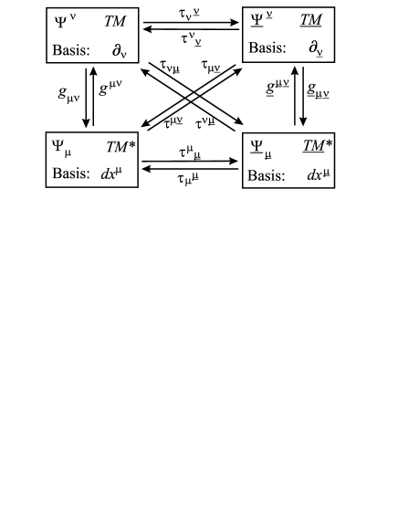
Figure 1: Relations between the maps. The left side depicts the tangential and co-tangential spaces. The right side depicts the corresponding spaces for the anti-gravitational fields.

The newly introduced field ${\underline{\Psi}}^{\underline{\kappa}}$ (from here on named anti-gravitating) transforms under local Lorentz-transformations like a Lorentz-vector in Special Relativity. But it differs in its behavior under general diffeomorphisms.

In order not to spoil the advantages of the Ricci-calculus, it will be useful to introduce a basis for the new fields that transforms accordingly. Locally, the new field can be expanded in this basis ${\partial}_{\underline{\kappa}}$. These basis elements form again a bundle on the manifold, that is denoted with ${\underline{TM}}$. To each of the elements of ${\underline{TM}}$ also a dual space exists, defined as the space of all linear maps on ${\underline{TM}}$. This space is denoted by ${\underline{TM}}^{*}$ and its basis as $d{{x}^{\underline{\kappa}}}$. The map from ${\underline{TM}}$ to ${\underline{TM}}^{*}$ will be denoted ${\underline{g}}_{{\underline{\kappa}}{\underline{\nu}}}$, and defines a scalar product on ${\underline{TM}}$.

Note, that the underlined indices on these quantities do not refer to the coordinates of the manifold but to the local basis in the tangential spaces. All of these fields still are functions of the space-time coordinates $x_{\nu}$.

$\tau$ maps the basis of one space into the other. We can expand it as $\tau=\tau_{\nu}^{\;\;{\underline{\kappa}}}~{}dx^{\nu}\partial_{\underline{\kappa}}$, or $\tau=\tau^{\nu}_{\;\;{\underline{\kappa}}}~{}dx^{\underline{\kappa}}\partial_{\nu}$ respectively, where we have introduced the inverse functions by

$$\tau_{\nu}^{\;\;{\underline{\kappa}}}\tau^{\nu}_{\;\;{\underline{\epsilon}}}=\delta^{\underline{\kappa}}_{\;\;\underline{\epsilon}}\quad,\quad\tau^{\epsilon}_{\;\;{\underline{\kappa}}}\tau_{\nu}^{\;\;{\underline{\kappa}}}=\delta^{\epsilon}_{\;\;\nu}\quad.$$ (6)

For completeness, let us also define the combined maps:

$$TM\longrightarrow{\underline{TM}}^{*} : \quad\tau_{\nu\underline{\nu}}=\tau_{\nu}^{\;\;{\underline{\kappa}}}{\underline{g}}_{{\underline{\kappa}}{\underline{\nu}}}\quad,\quad{{TM}}^{*}\longrightarrow{\underline{TM}}:\quad\tau^{\nu\underline{\nu}}=g^{\nu\kappa}\tau_{\kappa}^{\;\;\underline{\nu}}\quad.$$ (7)

As one sees from the transformation properties summarized in Eqs.(4), the map $\tau_{\nu\underline{\nu}}$ maps an element of $TM$ to its transponed. This transposition does not involve the metric tensor and is independent of the metric itself. In particular, one sees immediately that the determinant $|\tau_{\nu\underline{\nu}}|=1$, since transposition does not change the determinant.

Basis transformations in both spaces belong together, since their elements share the transformation properties Eqs.(4) with the same $G$. The map $\tau_{\nu\underline{\nu}}$ does not introduce an additional coordinate transformation in the underlined space, it does not change the volume element, introduce a shear, or an additional rotation on ${\underline{TM}}^{*}$. One should keep in mind that the introduction of the additional spaces is just a helpful tool to deal with the different transformation properties of the new fields.

The relation between the introduced quantities is summarized in Figure 1 from which we also read off the cycle leading back to identity on $TM^{*}$ and on ${\underline{TM}}^{*}$, respectively

$$\tau^{\kappa{\underline{\nu}}}{\underline{g}}{}_{{\underline{\kappa}}{\underline{\nu}}}\tau^{\nu{\underline{\kappa}}}g_{\nu\epsilon}=\delta^{\kappa}_{\;\epsilon}\quad,\quad{\underline{g}}{}^{{\underline{\kappa}}{\underline{\nu}}}\tau_{\nu{\underline{\kappa}}}g^{\kappa\nu}\tau_{\kappa{\underline{\epsilon}}}=\delta^{\underline{\kappa}}_{\;{\underline{\epsilon}}}\quad.$$ (8)

It is further helpful to note that $\tau$ can be expressed in a more intuitive form. Writing $\partial/\partial x^{\nu}=(\partial x^{\underline{\kappa}}/\partial x^{\nu})~{}\partial/\partial x^{\underline{\kappa}}$ one identifies

$$\tau^{\nu}_{\;\;\underline{\kappa}}=\frac{\partial x^{\nu}}{\partial x^{\underline{\kappa}}}\quad,$$ (9)

where we should keep in mind that $\partial_{\underline{\kappa}}$ is a just the basis in ${\underline{TM}}$ and does not correspond to an actual ’direction’ on the manifold as $\partial_{\nu}$ does.

The coordinate expansion of $\tau$ seems to depend on the basis chosen in ${TM}$ as well as on those in ${\underline{TM}}$. However, this ambiguity in the form of the map is only seemingly. The basis $\partial_{\nu}$ and ${\partial}_{\underline{\nu}}$ does not transform independently as stressed earlier. The relation between both basis transformations is fixed by the map $\tau$. To see this, note that even though the map $\tau$ for certain choices of coordinates might be trivial, its importance lies in its transformation behavior. Its covariant derivative takes into account the change of transformation behavior from $TM$ to ${\underline{TM}}$.

The transformation behavior in Eq. (5) together with the observation that in a locally orthonormal basis both fields transform identical under local Lorentz-transformations, gives us an explicit way to construct $\tau$. We choose a local orthonormal basis $\hat{e}$ in $TM$, which is related to the coordinate basis by the locally linear map $E\hat{e}=\partial$. In this basis, the metric is just $\eta$ and $\hat{\tau}$ is just the identity. One then finds $\tau$ in a general coordinate system by applying Eq.(5)

$$\tau=(E^{T})^{-1}\hat{\tau}E^{-1}=(EE^{T})^{-1}\quad.$$ (10)

Using Eq. (10), we again confirm that the determinant is $|\tau_{\kappa{\underline{\kappa}}}|=1$ and therefore

$$1 = g{\underline{g}}\quad,\quad|\tau_{\kappa}^{\;\;\underline{\kappa}}|=|g|\quad,\quad|\tau^{\kappa}_{\;\;\underline{\kappa}}|=|\underline{g}|\quad.$$ (11)

The properties of the vector-fields are transferred directly to those of fermionic fields by using the fermionic representation and transformations of $\tau$. In this case, the map $(\;)^{\dagger}\gamma^{0}$, instead of the metric, is used to relate a particle to the particle transforming under the contragredient representation.

It is now straightforward to introduce a covariant derivative for the new fields, in much the same way as one usually introduces the derivative for the charge-conjugated particles. We will use the notation $\nabla$ for the general-covariant derivative and $D$ for the general covariant derivative including the gauge-derivative of the fields. It is understood that the form of the derivative is defined by the field it acts on, even though this will not be noted explicitly.

Let us first introduce the derivative in the direction of $\nu$ on the basis in a general way by

$$\nabla_{\nu}\partial_{\kappa} = \Gamma^{\epsilon}_{\;\nu\kappa}~{}\partial_{\epsilon}\quad,\quad{\nabla}_{\nu}{\partial}_{\underline{\kappa}}=\Gamma^{{\underline{\epsilon}}}_{\;\;\nu{\underline{\kappa}}}~{}{\partial}_{\underline{\epsilon}}\quad.$$ (12)

We will further also use the notation

$$\nabla_{\underline{\kappa}}=\tau^{\kappa}_{\;\;\underline{\kappa}}\nabla_{\kappa}\quad\quad.$$ (13)

From Eqs. (12) it follows using the Leibniz-rule that

$$\nabla_{\nu}dx^{\kappa} = -\Gamma^{\kappa}_{\;\nu\epsilon}dx^{\epsilon}\quad,\quad{\nabla}_{\nu}dx^{{\underline{\kappa}}}=-\Gamma^{{\underline{\kappa}}}_{\;\;\nu{\underline{\epsilon}}}~{}dx^{\underline{\epsilon}}\quad.$$ (14)

So far, this is only a definition for the symbols $\Gamma^{\epsilon}_{\;\nu\kappa}$ and $\Gamma^{{\underline{\epsilon}}}_{\;\;\nu{\underline{\kappa}}}$. To get an explicit formula for these Christoffelsymbols one commonly uses the requirement that the covariant derivative on the metric itself vanishes. The geometrical meaning is that the scalar product is covariantly conserved. To keep the symmetry between both spaces, we require that also the scalar product of the new fields is conserved, that is $\nabla_{\lambda}g_{\nu\kappa}=0$ and $\nabla_{\lambda}{\underline{g}}_{\underline{\nu}\underline{\kappa}}=0$. Or, since $|\tau^{\lambda}_{\;\;\underline{\lambda}}|\neq 0$, the latter is with Eq.(13) equivalent to $\nabla_{\underline{\lambda}}g_{\underline{\nu}\underline{\kappa}}=0$. From this one finds in the usual way (see e.g. Ref.Weinberg )

$$\Gamma^{\nu}_{\;\;\lambda\kappa} = \frac{1}{2}g^{\nu\alpha}\left(\partial_{\lambda}g_{\kappa\alpha}+\partial_{\kappa}g_{\lambda\alpha}-\partial_{\alpha}g_{\kappa\lambda}\right)\quad,$$ (15)

$$\Gamma^{\underline{\nu}}_{\;\;\underline{\lambda}\underline{\kappa}} = \frac{1}{2}{\underline{g}}^{\underline{\nu}\underline{\alpha}}\left(\partial_{\underline{\lambda}}{\underline{g}}_{\underline{\kappa\alpha}}+\partial_{{\underline{\kappa}}}{\underline{g}}_{\underline{\lambda\alpha}}-\partial_{\underline{\alpha}}{\underline{g}}_{\underline{\kappa}\underline{\lambda}}\right)\quad.$$ (16)

Using that the Christoffelsymbols transform homogenously in the second index and removing the underlined derivatives we find

$$\Gamma^{\underline{\nu}}_{\;\;\lambda\underline{\kappa}} = \frac{1}{2}{\underline{g}}^{\underline{\nu}\underline{\alpha}}\left(\partial_{\lambda}{\underline{g}}_{\underline{\kappa\alpha}}+\tau_{\lambda}^{\;\;\underline{\lambda}}\tau^{\kappa}_{\;\;\underline{\kappa}}\partial_{{\kappa}}{\underline{g}}_{\underline{\lambda\alpha}}-\tau_{\lambda}^{\;\;\underline{\lambda}}\tau^{\alpha}_{\;\;\underline{\alpha}}\partial_{\alpha}{\underline{g}}_{\underline{\kappa}\underline{\lambda}}\right)\quad.$$ (17)

From this, one can explicitly compute the form of the derivatives in Eqs. (12).

At this point it is useful to state a general expectation about the connection coefficients. For a particle moving in a curved spacetime, it is possible to choose a freely falling coordinate system, in which the Christoffelsymbols in Eq.(15) vanish. However, this freely falling frame for the particle will in general not also be a freely falling frame for the anti-gravitational particle. Therefore, the Christoffelsymbols in Eq.(17) will not vanish in the freely falling frame of the usually gravitating particle. Both sets of symbols therefore will not be proportional to each other.

One further derives the useful relations

$$\nabla_{\nu}\tau_{\alpha\underline{\alpha}} = \partial_{\nu}\tau_{\alpha\underline{\alpha}}-\Gamma^{\kappa}_{\;\;\nu\alpha}\tau_{\kappa\underline{\alpha}}-\Gamma^{\underline{\kappa}}_{\;\;\nu\underline{\alpha}}\tau_{\alpha\underline{\kappa}}$$ (18)

$$\nabla_{\nu}\tau^{\alpha}_{\;\;\underline{\alpha}} = \partial_{\nu}\tau^{\alpha}_{\;\;\underline{\alpha}}+\Gamma^{\alpha}_{\;\;\nu\kappa}\tau^{\kappa}_{\;\;\underline{\alpha}}-\Gamma^{\underline{\kappa}}_{\;\;\nu\underline{\alpha}}\tau_{\alpha\underline{\kappa}}\quad.$$ (19)

With these covariant derivatives, one obtains the Lagrangian of the anti-gravitational field by replacing all quantities with the corresponding anti-gravitational quantities and using the appropriate derivative for the new fields to assure homogenous transformation behavior

$${\underline{\mathcal{L}}}={{\mathcal{L}}}(g_{\kappa\nu}\to{\underline{g}}{}_{{\underline{\kappa}}{\underline{\nu}}},\Psi\to{\underline{\Psi}})\quad,\quad{{\mathcal{L}}}={\underline{\mathcal{L}}}({\underline{g}}{}_{{\underline{\kappa}}{\underline{\nu}}}\to g_{\kappa\nu},{\underline{\Psi}}\to{\Psi})\quad.$$ (20)

To start with the most important example, the Lagrangian of fermionic fields can now be composed from the new ingredients as ${\mathcal{L}}^{\rm tot}_{F}={\mathcal{L}}_{F}+{\underline{\mathcal{L}}}_{F}$ with

$${\mathcal{L}}_{F} = ({D}/\hskip 4.26773pt\overline{\Psi})\Psi+{\overline{\Psi}}(D/\hskip 4.26773pt\Psi)\quad,\quad{\underline{\mathcal{L}}}_{F}=({{D}}/\hskip 4.26773pt{\underline{\overline{\Psi}}}){\underline{\Psi}}+{{\overline{\underline{\Psi}}}}({{D}}/\hskip 4.26773pt{\underline{{\Psi}}})\quad.$$ (21)

All other mixtures do not obey general covariance and/or gauge covariance.

The Lagrangian for anti-gravitational pendants ${\underline{A}}^{a}$ of the gauge fields is introduced via the field strength tensor

$${\underline{F}}^{a}_{{\underline{\kappa}\underline{\nu}}}=\nabla_{\underline{\kappa}}{\underline{A}}^{a}_{\underline{\nu}}-\nabla_{\underline{\nu}}{\underline{A}}^{a}_{\underline{\kappa}}+ef^{abc}{\underline{A}}_{\underline{\kappa}}^{b}{\underline{A}}_{\underline{\nu}}^{c}\quad,$$ (22)

where $f^{abc}$ are the structure constants of the group and $e$ is the coupling. One then constructs the Lagrangian from ${\underline{\mathcal{L}}}_{A}=-\frac{1}{4}{\rm Tr}\left({\underline{F}}^{\kappa\nu}{\underline{F}}_{\kappa\nu}\right)$. Again, a mixture of $F$ with the usual ${\underline{F}}$ is forbidden by gauge-symmetry. Note, that in all cases the kinetic energy terms are positive. A particle with negative gravitational mass behaves like an ordinary particle except for its gravitational interaction, encoded in the covariant derivatives.

As one sees by examining the Lagrangian, there is no direct interaction between gravitating and anti-gravitating particles. Nevertheless, both of the particle-species will interact with the gravitational field, which mediates an interaction between them. However, this coupling is suppressed with the Planck scale. Therefore, the production of anti-gravitating matter is not observable today because all ingoing particles, in whatever scattering process we look at, are the normally gravitating ones that we deal with every day.

3 Properties of Anti-Gravitating Matter

From the results of the last section, we can now write down the most general form of the Lagrangian which includes the anti-gravitating matter fields and is symmetric under exchange of gravitational with anti-gravitational quantities. It takes the form

$$S = \int{\rm d}^{d+4}x~{}\sqrt{-g}\left[G~{}R+{\mathcal{L}}+{\underline{\mathcal{L}}}\right]\quad,$$ (23)

where $G=1/m_{p}^{2}$, ${\mathcal{L}}={\mathcal{L}}_{F}+{\mathcal{L}}_{A}$, and ${\underline{\mathcal{L}}}={\underline{\mathcal{L}}}_{F}+{\underline{\mathcal{L}}}_{A}$.

After a variation of the metric, $\delta g_{\kappa\nu}$, the field equations read

$$R_{\kappa\nu}-\frac{1}{2}Rg_{\kappa\nu}=\frac{1}{G}\left(T_{\kappa\nu}+{\underline{T}}_{\kappa\nu}\right)\quad,$$ (24)

with the stress-energy tensors (SETs) as source terms

$$T^{\kappa\nu} = \frac{2}{\sqrt{-g}}\frac{\delta}{\delta g_{\kappa\nu}}\left(\sqrt{-g}{\mathcal{L}}\right)\quad,\quad{\underline{T}}^{\kappa\nu}=\frac{2}{\sqrt{-g}}\frac{\delta}{\delta g_{\kappa\nu}}\left(\sqrt{-{g}}{\underline{\mathcal{L}}}\right)\quad.$$ (25)

Using Eq.(20), and $g_{\kappa\nu}=\tau^{\kappa}_{\;\;\underline{\kappa}}\tau^{\nu}_{\;\;\underline{\kappa}}{\underline{g}}_{\underline{\kappa}\underline{\nu}}$, and performing the functional derivative, we find

$$\frac{\delta{\mathcal{L}}}{\delta g_{\kappa\nu}}=\tau^{\kappa}_{\;\;{\underline{\kappa}}}\tau^{\nu}_{\;\;{\underline{\nu}}}\frac{\delta{\underline{\mathcal{L}}}}{\delta{\underline{g}}{}_{{\underline{\kappa}}{\underline{\nu}}}}\quad.$$ (26)

We recall that $\tau_{\kappa{\underline{\nu}}}$ just transpones quantities and is independent of the metric tensor. It does not rotate the basis relative to each other, nor does it change the volume element or introduce a shear. Under a variation of the metric, this quantity remains unaltered $\delta\tau_{\kappa{\underline{\nu}}}=0$. This, however, is not the case for $\tau_{\kappa}^{\;\;{\underline{\nu}}}$, because it transforms non trivially under coordinate transformations which form a subset of the metric variations. In particular with Eq. (8) one obtains

$$\tau^{\kappa{\underline{\nu}}}~{}\tau_{\nu{\underline{\kappa}}}~{}\delta\left({\underline{g}}{}_{{\underline{\kappa}}{\underline{\nu}}}~{}g_{\nu\epsilon}\right)=0\quad,$$ (27)

and, after contraction with $\tau_{\kappa{\underline{\epsilon}}}~{}\tau_{\alpha}^{\;\;{\underline{\epsilon}}}$, this results in

$$\delta{g}_{\alpha\epsilon}+\tau_{\alpha}^{\;\;{\underline{\epsilon}}}~{}\tau_{\epsilon}^{\;\;{\underline{\kappa}}}~{}\delta{\underline{g}}{}_{{\underline{\kappa}}{\underline{\epsilon}}}=0\quad.$$ (28)

Inserting Eq. (28) in Eq. (26) yields

$$\frac{\delta{\mathcal{L}}}{\delta g_{\kappa\nu}}=-\frac{\delta{\underline{\mathcal{L}}}}{\delta{g}_{\kappa\nu}}\quad.$$ (29)

But the SET consists of two terms, the second one arising from the variation of the volume element. Using $\delta\sqrt{-g}=-\frac{1}{2}g_{\kappa\nu}\sqrt{-g}~{}\delta g^{\kappa\nu}$, one finds the SETs for the fields

$$T^{\kappa\nu} = \frac{\delta{\mathcal{L}}}{\delta{g}_{\kappa\nu}}-\frac{1}{2}g^{\kappa\nu}{\mathcal{L}}\quad,\quad{\underline{T}}^{\kappa\nu}=-\tau^{\kappa}_{\;\;{\underline{\kappa}}}\tau^{\nu}_{\;\;{\underline{\nu}}}\left(\frac{\delta{\underline{\mathcal{L}}}}{\delta{\underline{g}}_{{\underline{\kappa}}{\underline{\nu}}}}+\frac{1}{2}{\underline{g}}^{{\underline{\kappa}}{\underline{\nu}}}{\underline{\mathcal{L}}}\right)\quad.$$ (30)

The interpretation of the so derived gravitational SETs is straightforward: Under a perturbation of the metric, the anti-gravitational fields will undergo a transformation exactly opposite to these of the normal fields as one expects by construction. The $\tau$-functions convert the indices and the transformation behavior from ${\underline{TM}}$ to the usual tangential space.

Most importantly, we see that the SET of the anti-gravitating field yields a contribution to the source of the field equations with a minus sign (and thus justifies the name anti-gravitation). This is due to the modified transformation behavior of the field components. However, we also see that the second term, arising from the variation of the metric determinant, does not change sign. For one of the most important cases however, the fermionic matter field, the second term vanishes since the Lagrangian is zero when the field fulfills the equation of motion.

If one considers the Lagrangian of the Dirac-field one has to formulate the action in form of the tetrad fields. The above used argument then directly transfers to the Dirac field through the properties of the anti-gravitational field under diffeomorphisms. For the fermions, the SET then can be simplified inserting that the field fulfills the equations of motion $D/\hskip 4.26773pt\Psi=D/\hskip 4.26773pt\underline{\Psi}=0$.

The corresponding conservation law of the derived source terms as follows from the Bianchi-identities is as usual $\nabla^{\nu}(T_{\kappa\nu}+{\underline{T}}_{\kappa\nu})=0$.

By variation of the action Eq. (23) with respect to the fields, on obtains the equations of motion in form of the Euler-Lagrange equations. Using the the covariant form of Gauss’ law one finds as usual

$$\nabla_{\nu}\left(\frac{\partial{\mathcal{L}}}{\partial(\nabla_{\nu}\Psi)}\right)-\frac{\partial{\mathcal{L}}}{\partial\Psi}=0\quad.$$ (31)

In complete analogy to the usual case one derives the equations of motion for the anti-gravitational field

$${\nabla}_{\nu}\left(\frac{\partial{\underline{\mathcal{L}}}}{\partial({\nabla}_{\nu}{\underline{\Psi}})}\right)-\frac{\partial{\underline{\mathcal{L}}}}{\partial{\underline{\Psi}}}=0\quad.$$ (32)

For this derivation one can still use the usual covariant form of Gauss’ law since the derivatives $\nabla_{\nu}\underline{\Psi}$ transform as usual vectors with respect to the index $\nu$.

Now it is crucial to note that the kinetic SET as defined from the Noether current does not have a change in sign, as no variation of the metric is involved and the gravitational properties of the fields do not play a role. To clearly distinguish this canonical SET from the gravitational source term, let us denote the canonical SET with $\Theta_{\nu\kappa}$, whereas we keep the above used $T_{\nu\kappa}$ for the gravitational SET.

The canonical SET for a matter Lagrangian ${\mathcal{L}}(\Psi,\nabla_{\nu}\Psi)$ as follows from Noether’s theorem is

$$\Theta^{\nu}_{\;\;\kappa}=\frac{\partial{\mathcal{L}}}{\partial(\nabla_{\nu}\Psi)}\nabla_{\kappa}\Psi-\delta^{\nu}_{\;\;\kappa}{\mathcal{L}}\quad,$$ (33)

and is covariantly conserved $\nabla_{\nu}\Theta^{\nu}_{\;\;\kappa}=0$. Correspondingly one finds the conserved current for the anti-gravitational field

$${\underline{\Theta}}^{\nu}_{\;\;\underline{\kappa}}=\tau^{\kappa}_{\;\;\underline{\kappa}}\left(\frac{\partial{\mathcal{\underline{L}}}}{\partial({\nabla}_{\nu}{\underline{\Psi}})}{\nabla}_{\kappa}{\underline{\Psi}}-\delta^{\nu}_{\;\;\kappa}{\mathcal{\underline{L}}}\right)\quad,$$ (34)

which is also covariantly conserved $\nabla_{\nu}\underline{\Theta}^{\nu}_{\;\;\underline{\kappa}}=0$.

Unfortunately, in general these quantities are neither symmetric, nor are they traceless or gauge-invariant. For GR, Belinfante’s tensor is the more adequate one enmomt1 . Though the ’correct’ kinetic SET is a matter of ongoing discussion enmomt1 ; enmomt2 ; Babak:1999dc , the details will not be important for the following. Instead, let us note that, from the Noether current, we get a total conserved quantity for each space-time direction $\kappa$, leading to the conservation equations

$$\nabla^{\nu}\Theta_{\nu\kappa}+\tau_{\kappa}^{\;\;\underline{\kappa}}~{}{\nabla}^{\nu}{\underline{\Theta}}_{\nu\underline{\kappa}}=0\quad.$$ (35)

The form of the second term of Eq. (35) is readily interpreted: when the anti-gravitating particle gains kinetic energy on a world line, the gravitational particle would loose energy when traveling on the same world line. The interaction with the gravitational field is inverted.

One thus can identify the anti-gravitating particle as a particle whose kinetic momentum vector transforms under general diffeomorphism according to Eq.(4), whereas the standard particle’s kinetic momentum transforms according to Eq.(3).

It is also instructive to look at the motion of a classical test particle by considering the analogue of parallel-transporting the tangent vector. The particle’s world line is denoted ${x}_{\nu}(\lambda)$, and the anti-gravitating particle’s world line is denoted ${\underline{x}}_{\nu}(\lambda)$.

In contrast to the gravitating particle, the anti-gravitating particle parallel transports not its tangent vector ${\underline{t}}^{\alpha}=d{\underline{x}}^{\alpha}/d\lambda$, but instead the related quantity in ${\underline{TM}}$, which corresponds to the kinetic momentum, and is ${\underline{t}}^{\underline{\alpha}}=\tau_{\alpha}^{\;\;\underline{\alpha}}{\underline{t}}^{\alpha}$. On the particle’s world line ${\underline{x}}_{\nu}(\lambda)$, it is ${\underline{t}}^{\underline{\alpha}}$ which is covariantly conserved. Parallel transporting is then expressed in evaluating the derivative in direction of the curve and set it to zero. For the usual geodesic which parallel transports the tangential vector one has $t^{\nu}{\nabla}_{\nu}~{}{t}^{\alpha}=0$, whereas for the anti-gravitating particle one has

$${\underline{t}}^{\nu}~{}\tau^{\alpha}_{\;\;\underline{\alpha}}~{}{\nabla}_{\nu}~{}\tau_{\kappa}^{\;\;\underline{\alpha}}~{}{\underline{t}}^{\kappa}=0\quad,$$ (36)

which agrees with the usual equation if and only if the covariant derivative on $\tau_{\kappa}^{\;\;\underline{\alpha}}$ vanishes. It is important to note that the tangent vector ${\underline{t}}^{\alpha}$ is not parallel transported along the curve given by the new Eq. (36).

Using the covariant derivative ${\nabla}_{\nu}{\underline{t}}^{\underline{\alpha}}={\partial}_{\nu}{\underline{t}}^{\underline{\alpha}}+\Gamma^{{\underline{\alpha}}}_{\;\;{\nu}{\underline{\epsilon}}}~{}{\underline{t}}^{\underline{\epsilon}}$, from Eq.(14) one obtains

$$\frac{d{\underline{x}}^{\nu}}{d\lambda}\cdot\left(\partial_{\nu}\frac{d{\underline{x}}^{{\underline{\alpha}}}}{d\lambda}+\Gamma^{\underline{\alpha}}_{\;\;\nu\underline{\epsilon}}\frac{d{\underline{x}}^{\underline{\epsilon}}}{d\lambda}\right)=0\quad,$$ (37)

and by rewriting $\partial_{\nu}=(d\lambda/d{\underline{x}}^{\nu})~{}d/d\lambda$ one finds the anti-geodesic equation

$$\frac{d^{2}{\underline{x}}^{{\underline{\alpha}}}}{d\lambda^{2}}+\tau^{\nu}_{\;\;\underline{\nu}}\Gamma^{\underline{\alpha}}_{\;\;\nu\underline{\epsilon}}\frac{d{\underline{x}}^{{\underline{\epsilon}}}}{d\lambda}\frac{d{\underline{x}}^{{\underline{\nu}}}}{d\lambda}=0\quad.$$ (38)

This equation should be read as an equation for the quantity ${\underline{t}}^{\underline{\alpha}}$ rather than an equation for the curve. To obtain the curve, one proceeds as follows

• Integrate Eq. (38) once to obtain ${\underline{t}}^{\underline{\alpha}}$,

• Translate this into the geometric tangential vector ${\underline{t}}^{\underline{\alpha}}=\tau_{\alpha}^{\;\;\underline{\alpha}}{\underline{t}}^{\alpha}$,

• Integrate a second time with appropriate initial conditions to obtain ${\underline{x}}^{\alpha}$.

Alternatively, one can reformulate Eq. (36) directly into an equation for the tangential vector

$${\underline{t}}^{\nu}~{}{\nabla}_{\nu}~{}{\underline{t}}^{\alpha}+{\underline{t}}^{\nu}{\underline{t}}^{\kappa}~{}\tau^{\alpha}_{\;\;\underline{\alpha}}~{}{\nabla}_{\nu}~{}\tau_{\kappa}^{\;\;\underline{\alpha}}=0\quad,$$ (39)

and insert Eq.(19).

It will be instructive to also derive this anti-geodesic equation in a second way, which makes use of the energy conservation rather than postulating parallel transport. Let us look at an anti-gravitating test particle of nonzero but negative gravitational mass $m$ moving in a strong gravitational field. The particle’s energy conservation law Eq.(35) in the background field reads:

$$\partial_{\nu}~{}{\underline{\Theta}}^{\nu{\underline{\kappa}}}+\Gamma^{\underline{\kappa}}_{\;\;\nu\underline{\epsilon}}{\underline{\Theta}}^{\nu{\underline{\epsilon}}}+\Gamma^{\nu}_{\;\;\nu\epsilon}{\underline{\Theta}}^{\epsilon{\underline{\kappa}}}=0\quad.$$ (40)

The particle moves on the world line ${y}^{\nu}={x}^{\nu}(\lambda)$, where $\lambda={x}^{0}(\lambda)$ is the eigen time. For the particle of nonzero mass it can be used to parameterize the curve. The kinetic SET is then a function of $y$ and can be written as Weinberg

$${\underline{\Theta}}^{\nu\underline{\kappa}}(y) = m\int\frac{dx^{\nu}}{d\lambda}\frac{dx^{\underline{\kappa}}}{d\lambda}\frac{\delta^{4}({y}^{{\epsilon}}-{x}^{{\epsilon}}(\lambda))}{\sqrt{-g}}d\lambda\quad.$$ (41)

Taking the partial derivative with respect to $y_{\nu}$ and rewriting the derivative on the $\delta$-function yields

$$\frac{\partial}{\partial y^{\nu}}{\underline{\Theta}}^{\nu\underline{\kappa}}(y) = -m\int\frac{d\lambda}{\sqrt{-g}}\delta^{4}({y}^{{\epsilon}}-{x}^{{\epsilon}}(\lambda))\left[\frac{d^{2}x^{\underline{\kappa}}}{d\lambda^{2}}-\Gamma^{\epsilon}_{\;\;\epsilon\nu}\frac{dx^{\nu}}{d\lambda}\frac{dx^{\underline{\kappa}}}{d\lambda}\right]\quad.$$ (42)

Inserting Eq.(40) yields

$$0 = \int\frac{d\lambda}{\sqrt{-g}}\delta^{4}({y}^{{\epsilon}}-{x}^{{\epsilon}}(\lambda))\bigg{[}\frac{d^{2}x^{\underline{\kappa}}}{d\lambda^{2}}-\Gamma^{\epsilon}_{\;\;\epsilon\nu}\frac{dx^{\nu}}{d\lambda}\frac{dx^{\underline{\kappa}}}{d\lambda}+\Gamma^{\underline{\kappa}}_{\;\;\nu\underline{\epsilon}}\frac{dx^{\nu}}{d\lambda}\frac{dx^{\underline{\epsilon}}}{d\lambda}+\Gamma^{\nu}_{\;\;\nu\epsilon}\frac{dx^{\epsilon}}{d\lambda}\frac{dx^{\underline{\kappa}}}{d\lambda}\bigg{]},$$

where the second and the last term in the brackets cancel. Demanding that this be valid on the world line of the particle, one again finds Eq.(38).

On both our ways to derive this equation, we have not used one of the most common approaches which introduces the particle’s world line as the extremal of a variation of the length of the curve. Here we have instead solely used the consequences from a variation of the action Eq. (23) which includes geodesic motion as well as anti-geodesic motion.

It is important to note that the equations of motion Eq.(38) are invariant under general diffeomorphism, provided that the quantities are transformed appropriately. In case the space-time is globally flat, one can choose $g=\eta$. It is then also ${\underline{g}}=\eta$, and $\tau=$ Id, and both sets of Christoffelsymbols vanish. Since in this case both curves which describe the motion of the particles are identical, they will be identical for all choices of coordinate systems in a globally flat background.

4 Discussion

In the presence of strong curvature effects, one expects the interaction between both types of matter to become important. Since the anti-gravitating contribution to the source-term of the field equations is negative, the positive energy theorem can be violated. The implications of this feature for the possibility of singularity avoidance should be investigated further.

Furthermore, the existence of negative gravitational sources can allow gravity to be neutralized, which could be used the address the stabilization and compactification problem within the context of extra dimensions.

It should also be noted that the anti-gravitating particles do not alter the Hawking-radiation of black holes. The black hole horizon is a trapped surface only for usual photons, not for the anti-graviating ones. Indeed, it would be very puzzeling if a particle could be trapped by a source it is repelled by. Therefore, the anti-gravitating particles will not contribute to the Hawking flux.

5 Conclusions

We have introduced particles into the Standard Model that can cause negative gravitational sources. These particles are defined by their transformation behavior under general diffeomorphism. In flat space they obey the laws of Special Relativity. We thereby have relaxed the equivalence principle.

The number of particles in the Standard Model is doubled in this scenario: each particle has an anti-gravitating partner particle which only differs in its opposite reaction to the gravitational field. It is not necessary to have a negative kinetic energy term. We have shown that the interaction between gravitating and anti-gravitating matter is mediated solely by gravitation. It is therefore naturally very weak, explaining why we have not seen any anti-gravitating matter so far.

References

- (1) A. D. Linde, Phys.Lett. B 200, 272 (1988).
- (2) A. Linde, [arXiv:hep-th/0211048].
- (3) J. W. Moffat, [arXiv:hep-th/0507020].
- (4) D. E. Kaplan and R. Sundrum, [arXiv:hep-th/0505265].
- (5) H. Bondi, Rev. Mod. Phys. 29, 423-428 (1957).
- (6) I. Quiros, [arXiv:gr-qc/0411064].
- (7) A. Borde, L. H. Ford and T. A. Roman, Phys. Rev. D 65, 084002 (2002) [arXiv:gr-qc/0109061].
- (8) P. C. W. Davies and A. C. Ottewill, Phys. Rev. D 65, 104014 (2002) [arXiv:gr-qc/0203003].
- (9) S. Ray and S. Bhadra, Int. J. Mod. Phys. D 13, 555 (2004) [arXiv:gr-qc/0212120].
- (10) D. E. Rosenberg, [arXiv:astro-ph/0008166].
- (11) D. F. Torres, G. E. Romero and L. A. Anchordoqui, Mod. Phys. Lett. A 13, 1575 (1998) [arXiv:gr-qc/9805075].
- (12) V. M. Zhuravlev, D. A. Kornilov and E. P. Savelova, Gen. Rel. Grav. 36 (2004) 1719.
- (13) V. Faraoni, Phys. Rev. D 70, 081501 (2004) [arXiv:gr-qc/0408073].
- (14) N. Arkani-Hamed, P. Creminelli, S. Mukohyama and M. Zaldarriaga, JCAP 0404, 001 (2004) [arXiv:hep-th/0312100].
- (15) N. Arkani-Hamed, H. C. Cheng, M. A. Luty and S. Mukohyama, JHEP 0405, 074 (2004) [arXiv:hep-th/0312099].
- (16) N. Arkani-Hamed, H. C. Cheng, M. A. Luty, S. Mukohyama and T. Wiseman, [arXiv:hep-ph/0507120].
- (17) R. B. Mann and J. J. Oh, [arXiv:hep-th/0504172].
- (18) A. Krause and S. P. Ng, [arXiv:hep-th/0409241].
- (19) R. E. G. Saravi, J. Phys. A 37 (2004) 9573-9586, [arXiv:math-ph/0306020].
- (20) M. Forger and H. Römer, Ann. Phys. 309 (2004) 306-389, [arXiv:hep-th/0307199].
- (21) S. V. Babak and L. P. Grishchuk, Phys. Rev. D 61, 024038 (2000) [arXiv:gr-qc/9907027].
- (22) S. Weinberg, ’Gravitation and Cosmology ’: Wiley (July, 1972) .