Abstract

We relate the geometrical construction of (2+1)-spacetimes via grafting to phase space and Poisson structure in the Chern-Simons formulation of (2+1)-dimensional gravity with vanishing cosmological constant on manifolds of topology $\mathbb{R}\times S_{g}$, where $S_{g}$ is an orientable two-surface of genus $g>1$. We show how grafting along simple closed geodesics $\lambda$ is implemented in the Chern-Simons formalism and derive explicit expressions for its action on the holonomies of general closed curves on $S_{g}$. We prove that this action is generated via the Poisson bracket by a gauge invariant observable associated to the holonomy of $\lambda$. We deduce a symmetry relation between the Poisson brackets of observables associated to the Lorentz and translational components of the holonomies of general closed curves on $S_{g}$ and discuss its physical interpretation. Finally, we relate the action of grafting on the phase space to the action of Dehn twists and show that grafting can be viewed as a Dehn twist with a formal parameter $\theta$ satisfying $\theta^{2}=0$.

1 Introduction

(2+1)-dimensional gravity is of physical interest as a toy model for the (3+1)-dimensional case. It is used as a testing ground which allows one to investigate conceptual questions arising in the quantisation of gravity without being hindered by the technical complexity in higher dimensions. One of these questions is the problem of ”quantising geometry” or, more concretely, the problem of recovering geometrical objects with a clear physical interpretation from the gauge theory-like formulations used as a starting point for quantisation.

In (2+1)-dimensions, the relation between Einstein’s theory of gravity and gauge theory is more direct than in higher dimensional cases, since the theory takes the form of a Chern-Simons gauge theory. Depending on the value of the cosmological constant, vacuum solutions of Einstein’s equations of motion are flat or of constant curvature. The theory has only a finite number of physical degrees of freedom arising from the matter content and topology of the spacetime. This absence of local gravitational degrees of freedom manifests itself mathematically in the possibility to formulate the theory as a Chern-Simons gauge theory [1, 2] where the gauge group is the (2+1)-dimensional Poincaré group $P_{3}^{\uparrow}$, the group $SO(3,1)\cong SL(2,\mathbb{C})/\mathbb{Z}_{2}$ or $SO(2,2)\cong(SL(2,\mathbb{R})\times SL(2,\mathbb{R}))/\mathbb{Z}_{2}$, respectively, for cosmological constant $\Lambda=0$, $\Lambda>0$ and $\Lambda<0$.

The main advantage of the Chern-Simons formulation of (2+1)-dimensional gravity is that it allows one to apply gauge theoretical concepts and methods which give rise to an efficient description of phase space and Poisson structure. As Einstein’s equations of motion take the form of a flatness condition on the gauge field, physical states can be characterised by holonomies, and conjugation invariant functions of the holonomies form a complete set of physical observables. Starting with the work of Nelson and Regge [3, 4, 5, 7, 6], Martin [8] and of Ashtekar, Husain, Rovelli, Samuel and Smolin [9], the description of (2+1)-dimensional gravity in terms of holonomies and the associated gauge invariant observables has proven useful in clarifying the structure of its classical phase space as well as in quantisation. An overview of different approaches and results is given in [10].

The disadvantage of this approach is that it makes it difficult to recover the geometrical picture of a spacetime manifold and thereby complicates the physical interpretation of the theory. Except for cases where the holonomies take a particularly simple form such as static spacetimes and the torus universe, it is in general not obvious how the description of the phase space in terms of holonomies and associated gauge invariant observables gives rise to a Lorentz metric on a spacetime manifold. The first to address this problem for general spacetimes was Mess [11], who showed how the geometry of (2+1)-dimensional spacetimes can be reconstructed from a set of holonomies. More recent results on this problem are obtained in the papers by Benedetti and Guadagnini [12] and by Benedetti and Bonsante [13], which are going to be our main references. They describe the construction of evolving spacetimes from static ones via the geometrical procedure of grafting, which, essentially, consists of inserting small annuli along certain geodesics of the spacetime. As they establish a unified picture for all values of the cosmological constant and show how this change of geometry affects the holonomies, they clarify the relation between holonomies and spacetime geometry considerably.

However, despite these results, the problem of relating spacetime geometry and the description of phase space and Poisson structure in terms of holonomies has not yet been fully solved. The missing link is the role of the Poisson structure. A complete understanding of the gauge invariant observables must include a physical interpretation of the transformations on phase space they generate via the Poisson bracket. Conversely, to interpret the geometrical construction of evolving (2+1)-spacetimes via grafting as a physical transformation, one needs to determine how it affects phase space and Poisson structure.

This paper addresses these questions for (2+1)-gravity with vanishing cosmological constant on manifolds of topology $\mathbb{R}\times S_{g}$, where $S_{g}$ is an orientable two-surface of genus $g>1$. It relates the construction of evolving (2+1)-spacetimes via grafting along simple, closed curves to the description of the phase space in terms of holonomies and the associated gauge invariant observables. The main results can be stated as follows.

1. We show how grafting along a closed, simple geodesic is implemented in the Chern-Simons formulation of (2+1)-dimensional gravity. Using the parametrisation of the phase space in terms of holonomies given in [14, 15], we deduce explicit expressions for the action of grafting on the holonomies of general curves on $S_{g}$ and investigate its properties as a transformation on phase space.

2. We derive the Hamiltonian that generates this grafting transformation via the Poisson bracket. This Hamiltonian is one of the two basic gauge invariant observables associated to a closed curve on $S_{g}$ and obtained from the Lorentz component of its holonomy.

3. We demonstrate that there is a symmetry relation between the transformation of the observables associated to a curve $\eta$ under grafting along $\lambda$ and the transformation of the corresponding observables for $\lambda$ under grafting along $\eta$. Infinitesimally, this relation takes the form of a general identity for the Poisson brackets of certain observables associated to the two curves.

4. We show that the action of grafting in our description of the phase space is closely related to the action of (infinitesimal) Dehn twists investigated in an earlier paper [16]. Essentially, grafting can be viewed as a Dehn twist with a formal parameter $\theta$ satisfying $\theta^{2}=0$.

The paper is structured as follows. In Sect. 2 we introduce the relevant definitions and notation, present some background on the (2+1)-dimensional Poincaré group and on hyperbolic geometry and summarise the description of grafted (2+1)-spacetimes in [12, 13] for the case of grafting along multicurves.

In Sect. 3, we briefly review the Hamiltonian version of the Chern-Simons formulation of (2+1)-dimensional gravity. We discuss the role of holonomies and summarise the relevant results of [14, 15], in which phase space and Poisson structure are characterised by a symplectic potential on the manifold $(P_{3}^{\uparrow})^{2g}$ with different copies of $P_{3}^{\uparrow}$ standing for the holonomies of a set of generators of the fundamental group $\pi_{1}(S_{g})$.

Sect. 4 discusses the implementation of grafting along closed, simple geodesics in the Chern-Simons formalism. We show how the geometrical procedure of grafting in [12, 13] gives rise to a transformation on the extended phase space $(P_{3}^{\uparrow})^{2g}$ and derive formulas for its action on the holonomies of general elements of the fundamental group $\pi_{1}(S_{g})$.

Sect. 5 establishes the relation of grafting and Poisson structure. After expressing the symplectic potential on the extended phase space $(P_{3}^{\uparrow})^{2g}$ in terms of variables adapted to the grafting transformations, we show that these transformations are generated by gauge invariant Hamiltonians and therefore act as Poisson isomorphisms. We deduce a general symmetry relation between the Poisson brackets of certain observables associated to general closed curves on $S_{g}$.

In Sect. 6, we explore the link between grafting and Dehn twists. We review the results concerning Dehn twists derived in [16] and introduce a graphical procedure which allows one to determine the action of grafting on the holonomies of general closed curves on $S_{g}$. By means of this procedure, we then demonstrate that there is a close relation between the action of grafting and (infinitesimal) Dehn twists.

In Sect. 7 we illustrate the general results from Sect. 4 to 6 by applying them to a concrete example. Sect. 8 contains a summary of our results and concluding remarks.

2 Grafted (2+1) spacetimes with vanishing cosmological constant: the geometrical viewpoint

2.1 The (2+1)-dimensional Poincaré group

Throughout the paper we use Einstein’s summation convention. Indices are raised and lowered with the three-dimensional Minkowski metric $\eta=\text{diag}(1,-1,-1)$, and ${\mbox{\boldmath$x$}}\cdot{\mbox{\boldmath$y$}}$ stands for $\eta({\mbox{\boldmath$x$}},{\mbox{\boldmath$y$}})$.

In the following $L_{3}^{\uparrow}$ and $P_{3}^{\uparrow}=L_{3}^{\uparrow}\ltimes\mathbb{R}^{3}$ denote, respectively, the the (2+1)-dimensional proper orthochronous Lorentz and Poincaré group. We identify $\mathbb{R}^{3}$ and the Lie algebra $so(2,1)=\text{Lie}\;L_{3}^{\uparrow}$ as vector spaces. The action of $L_{3}^{\uparrow}$ on $\mathbb{R}^{3}$ in its matrix representation then agrees with its action on $so(2,1)$ via the adjoint action

$$\mathrm{Ad}(u){\mbox{\boldmath$p$}}=p^{a}\,uJ_{a}u^{-1}=u^{b}_{\;\;a}p^{a}J_{b}\qquad{\mbox{\boldmath$p$}}=(p^{0},p^{1},p^{2})\cong p^{a}J_{a},$$ (2.1)

where $J_{a}$, $a=0,1,2$, are the generators of $so(2,1)$. For notational consistency with earlier papers [14, 15, 16] considering more general gauge groups we will use the notation $\mathrm{Ad}(u){\mbox{\boldmath$p$}}$ throughout the paper and often do not distinguish notationally between elements of $so(2,1)$ and associated vectors in $\mathbb{R}^{3}$. With the parametrisation

$$(u,{\mbox{\boldmath$a$}})=(u,-\mathrm{Ad}(u){\mbox{\boldmath$j$}})\in P_{3}^{\uparrow}\qquad\qquad u\in L_{3}^{\uparrow},\;{\mbox{\boldmath$a$}},{\mbox{\boldmath$j$}}\in\mathbb{R}^{3},$$ (2.2)

the group multiplication in $P_{3}^{\uparrow}$ is then given by

$$(u_{1},{\mbox{\boldmath$a$}}_{1})\cdot(u_{2},{\mbox{\boldmath$a$}}_{2})=(u_{1}\cdot u_{2},{\mbox{\boldmath$a$}}_{1}+\mathrm{Ad}(u_{1}){\mbox{\boldmath$a$}}_{2})=(u_{1}\cdot u_{2},-\mathrm{Ad}(u_{1}u_{2})({\mbox{\boldmath$j$}}_{2}+\mathrm{Ad}(u_{2}^{-1}){\mbox{\boldmath$j$}}_{1})).$$ (2.3)

The Lie algebra of $P_{3}^{\uparrow}$ is $\text{Lie}\;P_{3}^{\uparrow}=iso(2,1)$. Denoting by $J_{a}$, $a=0,1,2$, the generators of $so(2,1)$ by $P_{a}$, $a=0,1,2$, the generators of the translations, and choosing the convention $\epsilon_{012}=1$ for the epsilon tensor, we have the Lie bracket

$$[P_{a},P_{b}]=0,\quad[J_{a},J_{b}]=\epsilon_{abc}J^{c},\quad[J_{a},P_{b}]=\epsilon_{abc}P^{c},$$ (2.4)

and a non-degenerate, $\mathrm{Ad}$-invariant bilinear form $\langle\,,\,\rangle$ on $iso(2,1)$ is given by

$$\langle J_{a},P^{b}\rangle=\delta_{a}^{b},\quad\langle J_{a},J_{b}\rangle=\langle P^{a},P^{b}\rangle=0.$$ (2.5)

We represent the generators of $so(2,1)$ by the matrices

$$(J_{a})_{bc}=-\epsilon_{abc}$$ (2.6)

and denote by $\exp:\;so(2,1)\rightarrow L_{3}^{\uparrow},\;p^{a}J_{a}\mapsto e^{p^{a}J_{a}}$ the exponential map for $L_{3}^{\uparrow}$. As this map is surjective, see for example [17, 18], elements of $L_{3}^{\uparrow}$ can be parametrised in terms of a vector ${\mbox{\boldmath$p$}}\in\mathbb{R}^{3}$ with $p^{0}\geq 0$ as

$$u=e^{-p^{a}J_{a}}.$$

Using expression (2.6) for the generators of $so(2,1)$ and setting

$$\hat{\mbox{\boldmath$p$}}=\tfrac{1}{m}{\mbox{\boldmath$p$}}\qquad\text{for}\;m^{2}:=|{\mbox{\boldmath$p$}}^{2}|\neq 0,$$ (2.7)

we find

$$u_{ab}=\begin{cases}\hat{p}_{a}\hat{p}_{b}+\cos m(\eta_{ab}-\hat{p}_{a}\hat{p}_{b})+\sin m\epsilon_{abc}\hat{p}^{c}&p^{a}p_{a}=m^{2}>0\\ \eta_{ab}+\epsilon_{abc}p^{c}+\tfrac{1}{2}p_{a}p_{b}&p^{a}p_{a}=0\\ -\hat{p}_{a}\hat{p}_{b}+\cosh m(\eta_{ab}+\hat{p}_{a}\hat{p}_{b})+\sinh m\epsilon_{abc}\hat{p}^{c}&p^{a}p_{a}=-m^{2}<0.\end{cases}$$ (2.8)

Elements $u=e^{-p^{a}J_{a}}\in L_{3}^{\uparrow}$ are called elliptic, parabolic and hyperbolic, respectively, if ${\mbox{\boldmath$p$}}^{2}>0$, ${\mbox{\boldmath$p$}}^{2}=0$ and ${\mbox{\boldmath$p$}}^{2}<0$. Note that the exponential map is not injective, since $e^{2\pi nJ_{0}}=1$ for $n\in\mathbb{Z}$. However, in this paper we will be concerned with hyperbolic elements, for which the parametrisation (2.8) in terms of a spacelike vector ${\mbox{\boldmath$p$}}=(p^{0},p^{1},p^{2})$ with $p^{0}\geq 0$ is unique.

A convenient way of describing the Lie algebra $iso(2,1)$ and the group $P_{3}^{\uparrow}$ has been introduced in [8]. It relies on a formal parameter $\theta$ with $\theta^{2}=0$ analogous to the one occurring in supersymmetry. With the definition

$$(P_{a})_{bc}=\theta(J_{a})_{bc}=-\theta\epsilon_{abc},$$ (2.9)

it follows that the commutator of the matrices $P_{a},J_{a}$, $a=0,1,2$, is the Lie bracket (2.4) of the (2+1)-dimensional Poincaré algebra. Definition (2.9) also allows one to parametrise elements of the group $P_{3}^{\uparrow}$. Identifying

$$(u,{\mbox{\boldmath$a$}})\cong(1+\theta a^{b}J_{b})u,$$ (2.10)

one obtains the multiplication law

$$(1+\theta a_{1}^{b}J_{b})u_{1}\cdot(1+\theta a_{2}^{c}J_{c})u_{2} =u_{1}u_{2}+\theta a_{1}^{b}J_{b}u_{1}u_{2}+\theta u_{1}a_{2}^{b}J_{b}u_{2}+\theta^{2}a_{1}^{b}J_{b}u_{1}a_{2}^{c}J_{c}u_{2}$$ (2.11)

$$=(1+\theta(a_{1}^{b}+u_{1}a_{2}^{b}J_{b}u_{1}^{-1}))u_{1}u_{2},$$

and with the identification (2.1) of $so(2,1)$ and $\mathbb{R}^{3}$ one recovers the group multiplication law (2.3). Furthermore, the introduction of the parameter $\theta$ makes it possible to express the exponential map $\exp:\;iso(2,1)\rightarrow P_{3}^{\uparrow}$ in terms of the exponential map $\exp:so(2,1)\rightarrow L_{3}^{\uparrow}$ for the (2+1)-dimensional Lorentz group by setting

$$e^{p^{a}J_{a}+k^{a}P_{a}}=e^{(p^{a}+\theta k^{a})J_{a}}=\sum_{n=0}^{\infty}\frac{(p^{a}J_{a})^{n}}{n!}+\theta\sum_{n=0}^{\infty}\sum_{m=0}^{n-1}\frac{(p^{a}J_{a})^{m}(k^{b}J_{b})(p^{c}J_{c})^{n-m-1}\!\!\!\!\!\!\!\!\!\!\!\!\!\!\!}{n!}.$$ (2.12)

To link the parametrisation of elements of $P_{3}^{\uparrow}$ in terms of the exponential map with the parametrisation (2.2)

$$(u,-\mathrm{Ad}(u){\mbox{\boldmath$j$}})=e^{-(p^{a}+\theta k^{a})J_{a}}\qquad u\in L_{3}^{\uparrow},{\mbox{\boldmath$j$}}\in\mathbb{R}^{3},(p^{a}+\theta k^{a})J_{a}\in iso(2,1),$$ (2.13)

one uses the identity

$$[(p^{a}J_{a})^{n},k^{b}J_{b}]=\sum_{m=1}^{n}\left(\begin{array}[]{l}n\\ m\end{array}\right)\mathrm{ad}_{p^{a}J_{a}}^{m}(k^{b}J_{b})\cdot(p^{c}J_{c})^{n-m}$$ (2.16)

in (2.12) and finds that the elements $u\in L_{3}^{\uparrow}$, ${\mbox{\boldmath$j$}}\in\mathbb{R}^{3}$ are given by

$$u=e^{-p^{a}J_{a}},{\mbox{\boldmath$j$}}=T({\mbox{\boldmath$p$}}){\mbox{\boldmath$k$}}\quad\text{with}\;T:\mathbb{R}^{3}\rightarrow\mathbb{R}^{3}$$ (2.17)

$$T({\mbox{\boldmath$p$}})^{ab}k_{b}J_{a}=\sum_{n=0}^{\infty}\frac{\mathrm{ad}_{p^{a}J_{a}}^{n}(k^{a}J_{a})}{(n+1)!}=k^{a}J_{a}+\tfrac{1}{2}[p^{b}J_{b},k^{a}J_{a}]+\tfrac{1}{6}[p^{c}J_{c},[p^{b}J_{b},k^{a}J_{a}]]+\ldots.$$ (2.18)

Note that the linear map $T({\mbox{\boldmath$p$}})$ is the same as the one considered in [14, 15], where its properties are discussed in more detail. In particular, it is shown that $T({\mbox{\boldmath$p$}})$ is bijective, maps $p$ to itself and satisfies $\mathrm{Ad}(e^{-p^{a}J_{a}})T({\mbox{\boldmath$p$}})=T(-{\mbox{\boldmath$p$}})$. Its inverse $T^{-1}({\mbox{\boldmath$p$}}):\mathbb{R}^{3}\rightarrow\mathbb{R}^{3}$ plays an important role in the parametrisation of the right- and left-invariant vector fields $J^{L}_{a},J^{R}_{a}$ on $L_{3}^{\uparrow}$. For any $F\in\mathcal{C}^{\infty}(L_{3}^{\uparrow})$, we have

$$J_{a}^{L}F(e^{-p^{b}J_{b}})=\frac{d}{dt}|_{t=0}F(e^{-tJ_{a}}e^{-p^{b}J_{b}})=T^{-1}({\mbox{\boldmath$p$}})^{ab}\frac{\partial F}{\partial p^{b}}$$ (2.19)

$$J_{a}^{R}F(e^{-p^{b}J_{b}})=\frac{d}{dt}|_{t=0}F(e^{-p^{b}J_{b}}e^{tJ_{a}})=-\mathrm{Ad}(e^{p^{b}J_{b}})^{a}_{\;\;c}T^{-1}({\mbox{\boldmath$p$}})^{cb}\frac{\partial F}{\partial p^{b}}=-T^{-1}(-{\mbox{\boldmath$p$}})^{ab}\frac{\partial F}{\partial p^{b}}.$$

2.2 Hyperbolic geometry

In this subsection we summarise some facts from hyperbolic geometry, mostly following the presentation in [19]. For a more specialised treatment focusing on Fuchsian groups see also [20].

In the following we denote by $H_{T}\subset\mathbb{R}^{3}$ the hyperboloids of curvature $-\frac{1}{T}$ with the metric induced by the (2+1)-dimensional Minkowski metric

$$H_{T}=\{{\mbox{\boldmath$x$}}\in\mathbb{R}^{3}\;|\,{\mbox{\boldmath$x$}}^{2}=T^{2},\;x^{0}>0\}$$ (2.20)

and realise hyperbolic space $\mathbb{H}^{2}$ as the hyperboloid $\mathbb{H}^{2}=H_{1}$. The tangent plane in a point ${\mbox{\boldmath$p$}}\in H_{T}$ is given by

$$T_{\!{}_{\footnotesize{\mbox{\boldmath$p$}}}}H_{T}={\mbox{\boldmath$p$}}^{\bot}=\{{\mbox{\boldmath$x$}}\in\mathbb{R}^{3}\;|\;{\mbox{\boldmath$x$}}\cdot{\mbox{\boldmath$p$}}=0\},$$ (2.21)

and geodesics on $H_{T}$ are of the form

$${\mbox{\boldmath$c$}}_{p,q}(t)={\mbox{\boldmath$p$}}\cosh t+{\mbox{\boldmath$q$}}\sinh t\qquad\text{with}\;{\mbox{\boldmath$p$}}^{2}=T^{2},\,{\mbox{\boldmath$q$}}^{2}=-T^{2},\,{\mbox{\boldmath$p$}}\cdot{\mbox{\boldmath$q$}}=0.$$ (2.22)

They are given as the intersection of $H_{T}$ with planes through the origin, which can be characterised in terms of their unit (Minkowski) normal vectors

$${\mbox{\boldmath$c$}}_{p,q}=H_{T}\cap{\mbox{\boldmath$n$}}_{p,q}^{\bot}\qquad\text{with}\qquad{\mbox{\boldmath$n$}}_{p,q}=\tfrac{1}{T^{2}}{\mbox{\boldmath$p$}}\times{\mbox{\boldmath$q$}}\in T_{\!{}_{{\mbox{\boldmath$c$}}_{p,q}(t)}}H_{T}\;\forall t\in\mathbb{R}.$$ (2.23)

The isometry group of the hyperboloids $H_{T}$ is the (2+1)-dimensional proper orthochronous Lorentz group $L_{3}^{\uparrow}$. The subgroup stabilising a given geodesic maps the associated plane to itself and is generated by the plane’s normal vector. More precisely, for a geodesic ${\mbox{\boldmath$c$}}_{p,q}$ parametrised as in (2.22) and with associated normal vector ${\mbox{\boldmath$n$}}_{p,q}$ as in (2.23), one has

$$\mathrm{Ad}(e^{\alpha n_{p,q}^{a}J_{a}}){\mbox{\boldmath$c$}}_{p,q}(t)= \cosh(t+\alpha){\mbox{\boldmath$p$}}+\sinh(t+\alpha){\mbox{\boldmath$q$}}\qquad\alpha\in\mathbb{R}.$$ (2.24)

The uniformization theorem implies that any compact, oriented two-manifold of genus $g>1$ with a metric of constant negative curvature is given as a quotient $S_{\Gamma}=H_{T}/\Gamma$ of a hyperboloid $H_{T}$ by the action of a cocompact Fuchsian group with $2g$ hyperbolic generators

$$\Gamma=\langle v_{A_{1}},v_{B_{1}},\ldots,v_{A_{g}},v_{B_{g}};[v_{B_{g}},v_{A_{g}}^{-1}]\cdots[v_{B_{1}},v_{A_{1}}^{-1}]=1\rangle\subset L_{3}^{\uparrow}.$$ (2.25)

The group $\Gamma$ is isomorphic to the fundamental group $\pi_{1}(S_{\Gamma})$, and its action on the hyperboloid $H_{T}$ agrees with the action of $\pi_{1}(S_{\Gamma})$ via deck transformations. Via its action on $H_{T}$, it induces a tesselation of $H_{T}$ by its fundamental regions which are geodesic arc $4g$-gons. In particular, there exists a geodesic arc $4g$-gon $P_{\Gamma}^{T}$ in the tesselation of $H_{T}$, in the following referred to as fundamental polygon, such that each of the generators of $\Gamma$ and their inverses map the polygon to one of its $4g$ neighbours. If one labels the sides of the polygon by $a_{1},a_{1}^{\prime},\ldots,b_{1},b^{\prime}_{1},\ldots,a_{g},a_{g}^{\prime},b_{g},b_{g}^{\prime}$ as in Fig. 5, it follows that the generators of $\Gamma$ map side $x\in\{a_{1},\ldots,b_{g}\}$ of the polygon $P_{\Gamma}$ into $x^{\prime}\in\{a^{\prime}_{1},\ldots,b^{\prime}_{g}\}$

$$\mathrm{Ad}(v_{A_{i}}):a_{i}\rightarrow a_{i}^{\prime}\qquad\mathrm{Ad}(v_{B_{i}}):b_{i}\rightarrow b_{i}^{\prime}.$$ (2.26)

For a general polygon $P^{\prime}$ in the tesselation related to $P_{\Gamma}^{T}$ via $P^{\prime}=\mathrm{Ad}(v)P_{\Gamma}^{T}$, $v\in\Gamma$, the elements of $\Gamma$ mapping this polygon into its $4g$ neighbours are given by $vv_{A_{1}}^{\pm 1}v^{-1},\ldots,vv_{B_{g}}^{\pm 1}v^{-1}$.

Geodesics on $S_{\Gamma}$ are the images of geodesics on $H_{T}$ under the projection $\Pi_{\Gamma}^{T}:H_{T}\rightarrow S_{\Gamma}$. In particular, a geodesic ${\mbox{\boldmath$c$}}_{p,q}$ on $H_{T}$ gives rise to a closed geodesic on $S_{\Gamma}$ if and only if there exists a nontrivial element $\tilde{v}\in\Gamma$, the geodesic’s holonomy, which maps ${\mbox{\boldmath$c$}}_{p,q}$ to itself. From (2.24) it then follows that the group element $\tilde{v}\in\Gamma$ is obtained by exponentiating a multiple of the geodesic’s normal vector

$$\exists\alpha\in\mathbb{R}^{+}:\qquad\tilde{v}=e^{\alpha n_{p,q}^{a}J_{a}}.$$ (2.27)

Closed geodesics on $S_{\Gamma}$ are therefore in one to one correspondence with elements of the group $\Gamma$ and hence with elements of the fundamental group $\pi_{1}(S_{\Gamma})$. In the following we will often not distinguish notationally between an element of the fundamental group $\pi_{1}(S_{\Gamma})$ and a closed geodesic or a general closed curve on $S_{\Gamma}$ representing this element.

2.3 Grafting

Grafting along simple geodesics was first investigated in the context of complex projective structures and Teichmüller theory [21, 22, 23]. Following the work of Thurston [24, 25] who considered general geodesic laminations, the topic has attracted much interest in mathematics, for historical remarks see for instance [26]. The role of geodesic laminations in (2+1)-dimensional gravity was first explored by Mess [11] who investigated the construction of (2+1)-dimensional spacetimes from a set of holonomies. More recent work on grafting in the context of (2+1)-dimensional gravity are the papers by Benedetti and Guadagnini [12] and by Benedetti and Bonsante [13]. As we investigate a rather specific situation, namely grafting along closed, simple geodesics in (2+1)-dimensional gravity with vanishing cosmological constant $\Lambda$, we limit our presentation to a summary of the grafting procedure described in [12, 13] for the case of $\Lambda=0$ and multicurves. For a more general treatment and a discussion of the relation between this grafting procedure and grafting on the space of complex projective structures, we refer the reader to [12, 13].

Given a cocompact Fuchsian group $\Gamma$ with $2g$ generators, there is a well-known procedure for constructing a flat (2+1)-dimensional spacetime of genus $g$ associated to this group, see for example [10]. One foliates the interior of the forward lightcone with the tip at the origin by hyperboloids $H_{T}$. The cocompact Fuchsian group $\Gamma$ acts on each hyperboloid $H_{T}$ and induces a tesselation of $H_{T}$ by geodesic arc $4g$-gons which are mapped into each other by the elements of $\Gamma$. The asssociated spacetime of genus $g$ is then obtained by identifying on each hyperboloid the points related by the action of $\Gamma$. It is shown in [10] that the $P_{3}^{\uparrow}$-valued holonomies of all curves in the resulting spacetime have vanishing translational components and lie in the subgroup $L_{3}^{\uparrow}\subset P_{3}^{\uparrow}$. However, these spacetimes are of limited physical interest because they are static [10].

Grafting along measured geodesic laminations is a procedure which allows one to construct non-static or genuinely evolving (2+1)-spacetimes associated to a Fuchsian group $\Gamma$. In the following we consider measured geodesic laminations which are weighted multicurves, i. e.  countable or finite sets

$$G_{I}^{\Gamma}=\{(c_{i}^{\Gamma},w_{i})\;|\;i\in I\}$$ (2.28)

of closed, simple non-intersecting geodesics $c_{i}^{\Gamma}$ on the associated two-surface $S_{\Gamma}=\mathbb{H}^{2}/\Gamma$, each equipped with a positive number, the weight $w_{i}>0$.

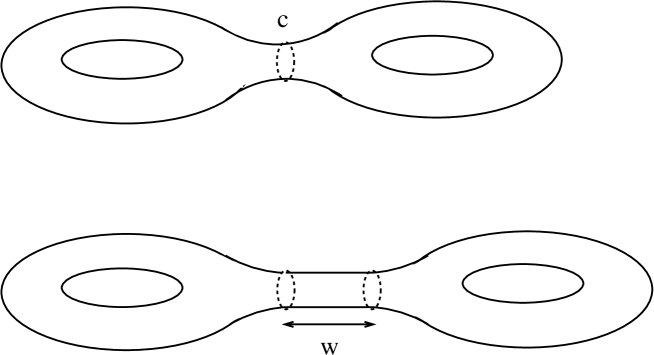
Figure 1: Grafting along a closed simple geodesic $c$ with weight $w$ on a genus 2 surface.

Geometrically, grafting amounts to cutting the surface $S_{\Gamma}$ along each geodesic $c_{i}$ and inserting a strip of width $w_{i}$ as indicated in Fig. 1.

hyper.eps

Figure 2: Grafting along a geodesic with weight $w$ in hyperbolic space.

Equivalently, the construction can be described in the universal cover $\mathbb{H}^{2}$. By lifting each geodesic $c_{i}^{\Gamma}$ to a geodesic ${\mbox{\boldmath$c$}}_{i}$ on $\mathbb{H}^{2}$ and acting on it with the Fuchsian group $\Gamma$, one obtains a $\Gamma$-invariant multicurve on $\mathbb{H}^{2}$

$$G_{I}=\{(\mathrm{Ad}(v){\mbox{\boldmath$c$}}_{i},w_{i})\,|\,i\in I,v\in\Gamma\}.$$ (2.29)

One then cuts the hyperboloid $\mathbb{H}^{2}$ along each geodesic $c_{i}$ in $G_{I}$, shifts the resulting pieces in the direction of the geodesics’ normal vectors and glues in a strip of width $w_{i}$ as shown in Fig. 2. The cocompact Fuchsian group $\Gamma$ acts on the resulting surface in such a way that it identifies the images of the points related by the canonical action of $\Gamma$ on $\mathbb{H}^{2}$, and the associated grafted genus $g$ surface is obtained by taking the quotient with respect to this action of $\Gamma$.

In the construction of flat (2+1)-spacetimes of topology $\mathbb{R}\times S_{g}$ via grafting, the grafting procedure is performed for each value of the time parametrising $\mathbb{R}$. As in the construction of static spacetimes, one foliates the interior of the forward lightcone by hyperboloids $H_{T}$. By cutting and inserting strips along the lifted geodesics on each hyperboloid $H_{T}$, one assigns to each cocompact Fuchsian group $\Gamma$ and each multicurve on $S_{\Gamma}=\mathbb{H}^{2}/\Gamma$ a regular domain $U\in\mathbb{R}^{3}$. The cocompact Fuchsian group $\Gamma$ acts on the domain $U$, and the grafted spacetime of topology $\mathbb{R}\times S_{g}$ is obtained by identifying the points in $U$ related by this action of $\Gamma$.

To give a mathematically precise definition, we follow the presentation in [13]. We consider a multicurve on $S=\mathbb{H}^{2}/\Gamma$ as in (2.28) together with its lift to a $\Gamma$-invariant weighted multicurve on $\mathbb{H}^{2}$ as in (2.29) and parametrise its geodesics as in (2.22)

$$G_{I}=\{({\mbox{\boldmath$c$}}_{p_{i},q_{i}},w_{i})\;|\;i\in I\}.$$ (2.30)

Furthermore, we choose a basepoint ${\mbox{\boldmath$x$}}_{0}\in\mathbb{H}^{2}-\bigcup_{i\in I}{\mbox{\boldmath$c$}}_{p_{i},q_{i}}$ that does not lie on any of the geodesics. For each point ${\mbox{\boldmath$x$}}\in\mathbb{H}^{2}-\bigcup_{i\in I}{\mbox{\boldmath$c$}}_{p_{i},q_{i}}$ outside the geodesics, we choose an arc ${\mbox{\boldmath$a$}}_{x}$ connecting ${\mbox{\boldmath$x$}}_{0}$ and $x$, pointing towards $x$ and transverse to each of the geodesics it intersects. We then define a map $\rho:\mathbb{H}^{2}-\bigcup_{i\in I}{\mbox{\boldmath$c$}}_{p_{i},q_{i}}\rightarrow\mathbb{R}^{3}$ by associating to each intersection point of ${\mbox{\boldmath$a$}}_{x}$ with one of the geodesics the unit normal vector of the geodesic pointing towards $x$ and multiplied with the weight

$$\rho({\mbox{\boldmath$x$}})=\!\!\!\!\!\!\!\!\!\!\!\!\!\!\sum_{i\in I:\;{\mbox{\boldmath$a$}}_{x}\cap{\mbox{\boldmath$c$}}_{p_{i},q_{i}}\neq\emptyset}\!\!\!\!\!\!\!\!\!\!\!\!w_{i}\epsilon_{i,x}{\mbox{\boldmath$n$}}_{p_{i},q_{i}}\qquad\text{for}\;{\mbox{\boldmath$x$}}\notin\bigcup_{i\in I}{\mbox{\boldmath$c$}}_{p_{i},q_{i}},$$ (2.31)

where $\epsilon_{i,x}\in\{\pm 1\}$ is the oriented intersection number of ${\mbox{\boldmath$a$}}_{x}$ and ${\mbox{\boldmath$c$}}_{p_{i},q_{i}}$ with the convention $\epsilon_{i,x}=1$ if ${\mbox{\boldmath$c$}}_{p_{i},q_{i}}$ crosses ${\mbox{\boldmath$a$}}_{x}$ from the left to the right in the direction of ${\mbox{\boldmath$a$}}_{x}$ and ensures that $\epsilon_{i,x}w_{i}{\mbox{\boldmath$n$}}_{p_{i},q_{i}}$ points towards $x$. Similarly, for each point ${\mbox{\boldmath$x$}}\in{\mbox{\boldmath$c$}}_{p_{j},q_{j}}$ that lies on one of the geodesics, we consider a geodesic ray ${\mbox{\boldmath$r$}}_{x}$ starting in ${\mbox{\boldmath$x$}}_{0}$ and through $x$, transversal to the geodesics at each intersection point, and set

$$\rho_{-}({\mbox{\boldmath$x$}})=\!\!\!\!\!\!\!\!\!\!\!\!\!\!\sum_{i\in I-\{j\}:\;{\mbox{\boldmath$r$}}_{x}\cap{\mbox{\boldmath$c$}}_{p_{i},q_{i}}\neq\emptyset}\!\!\!\!\!\!\!\!\!\!\!\!\!\!\!\!w_{i}\epsilon_{i,x}{\mbox{\boldmath$n$}}_{p_{i},q_{i}} \rho_{+}({\mbox{\boldmath$x$}})=w_{j}\epsilon_{j,x}{\mbox{\boldmath$n$}}_{p_{j}q_{j}}+\!\!\!\!\!\!\!\!\!\!\!\!\!\!\sum_{i\in I-\{j\}:\;{\mbox{\boldmath$r$}}_{x}\cap{\mbox{\boldmath$c$}}_{p_{i},q_{i}}\neq\emptyset}\!\!\!\!\!\!\!\!\!\!\!\!\!\!\!\!w_{i}\epsilon_{i,x}{\mbox{\boldmath$n$}}_{p_{i},q_{i}}.$$ (2.32)

On each hyperboloid $H_{T}$, we now shift the points outside of the geodesics according to

$$T{\mbox{\boldmath$x$}}\mapsto T{\mbox{\boldmath$x$}}+\rho({\mbox{\boldmath$x$}})\qquad{\mbox{\boldmath$x$}}\in\mathbb{H}^{2}-\bigcup_{i\in I}{\mbox{\boldmath$c$}}_{p_{i}q_{i}}$$ (2.33)

and replace each geodesic by a strip

$$T{\mbox{\boldmath$x$}}\mapsto T{\mbox{\boldmath$x$}}+t\rho_{+}({\mbox{\boldmath$x$}})+(1-t)\rho_{-}({\mbox{\boldmath$x$}})\qquad{\mbox{\boldmath$x$}}\in\bigcup_{i\in I}{\mbox{\boldmath$c$}}_{p_{i}q_{i}}\subset\mathbb{H}^{2},t\in[0,1].$$ (2.34)

From the definitions (2.31), (2.32) of the maps $\rho,\rho_{\pm}$ we see that for each value of $T$, this corresponds to the grafting procedure for hyperbolic space described above. The regular domain $U\subset\mathbb{R}^{3}$ associated to the multicurve $G_{I}$ is the image of the forward lightcone under this procedure [13]

$$U=\bigcup_{T\in\mathbb{R}^{+}}U_{T}$$ (2.35)

$$U_{T}=\underbrace{\left\{T{\mbox{\boldmath$x$}}+\rho({\mbox{\boldmath$x$}})\;|\;{\mbox{\boldmath$x$}}\notin\bigcup_{i\in I}{\mbox{\boldmath$c$}}_{p_{i},q_{i}}\right\}}_{=:U_{T}^{0}}\cup\underbrace{\left\{T{\mbox{\boldmath$x$}}+t\rho_{+}({\mbox{\boldmath$x$}})+(1-t)\rho_{-}({\mbox{\boldmath$x$}})\;|\;{\mbox{\boldmath$x$}}\in\bigcup_{i\in I}{\mbox{\boldmath$c$}}_{p_{i},q_{i}}\,,\;t\in[0,1]\right\}}_{=:U_{T}^{G_{I}}},$$

where the two-dimensional surfaces $U_{T}$ are the images of the hyperboloids $H_{T}$, given as a union of shifted pieces $U_{T}^{0}$ of hyperboloids and of strips $U_{T}^{G_{I}}$. In particular, the tip of the lightcone is mapped to the initial singularity $U_{0}$ of the regular domain $U$

$$U_{0}= \left\{\rho({\mbox{\boldmath$x$}})\;|\;{\mbox{\boldmath$x$}}\notin\bigcup_{i\in I}{\mbox{\boldmath$c$}}_{p_{i},q_{i}}\right\}\cup\left\{t\rho_{+}({\mbox{\boldmath$x$}})+(1-t)\rho_{-}({\mbox{\boldmath$x$}})\;|\;{\mbox{\boldmath$x$}}\in\bigcup_{i\in I}{\mbox{\boldmath$c$}}_{p_{i},q_{i}}\,,\;t\in[0,1]\right\},$$ (2.36)

which is a graph (more precisely, a real simplicial tree) with each vertex corresponding to the area between two geodesics or between a geodesic and infinity and edges given by $w_{i}\epsilon_{i,x}{\mbox{\boldmath$n$}}_{p_{i},q_{i}}$.

It is shown in [12] that the parameter $T$ defines a cosmological time function $T_{c}:U\rightarrow\mathbb{R}^{+}$

$$T_{c}(T{\mbox{\boldmath$x$}}+\rho({\mbox{\boldmath$x$}}))=T\quad T_{c}(T{\mbox{\boldmath$x$}}+t\rho_{+}({\mbox{\boldmath$x$}})+(1-t)\rho_{-}({\mbox{\boldmath$x$}}))=T,$$ (2.37)

and that the surfaces $U_{T}$ in (2.35) are surfaces of constant geodesic distance to the initial singularity $U_{0}$.

The genus $g$ spacetime associated to the cocompact Fuchsian group $\Gamma$ and the $\Gamma$-invariant multicurve $G_{I}$ is then obtained by identifying on each surface $U_{T}$ the images of the points on $H_{T}$ which are related by the canonical action of $\Gamma$. This is implemented by defining another action of the group $\Gamma$ on $U$. It is shown in [13] that for $\Gamma$-invariant multicurves $G_{I}$ on $\mathbb{H}^{2}$ the map

$$f_{G_{I}}:\Gamma\rightarrow P_{3}^{\uparrow},\;\;f_{G_{I}}(v)=(v,\rho(\mathrm{Ad}(v){\mbox{\boldmath$x$}}_{0}))$$ (2.38)

defines a group homomorphism which leaves each surface $U_{T}$ invariant, acts on $U$ freely and properly discontinuously and satisfies

$$N(f_{G_{I}}(v){\mbox{\boldmath$y$}})=\mathrm{Ad}(v)N({\mbox{\boldmath$y$}}),$$ (2.39)

where $N:U\rightarrow\mathbb{H}^{2}$ is the map that associates to each point in $U$ the corresponding point in $\mathbb{H}^{2}$

$$N(T{\mbox{\boldmath$x$}}+\rho({\mbox{\boldmath$x$}}))={\mbox{\boldmath$x$}}\quad N(T{\mbox{\boldmath$x$}}+t\rho_{+}({\mbox{\boldmath$x$}})+(1-t)\rho_{-}({\mbox{\boldmath$x$}}))={\mbox{\boldmath$x$}}.$$ (2.40)

The flat (2+1)-spacetime of genus $g$ associated to the group $\Gamma$ and the multicurve $G^{\Gamma}_{I}$ is defined as the quotient of $U$ by the action of $\Gamma$ via $f_{G_{I}}$. Using the identity (2.39), we find that this amounts to identifying points ${\mbox{\boldmath$y$}},{\mbox{\boldmath$y$}}^{\prime}\in\bigcup_{T\in\mathbb{R}^{+}}U_{T}^{0}$ according to

$${\mbox{\boldmath$y$}}\sim{\mbox{\boldmath$y$}}^{\prime}\quad\Leftrightarrow\quad\exists v\in\Gamma:\;N({\mbox{\boldmath$y$}})=\mathrm{Ad}(v)N({\mbox{\boldmath$y$}}^{\prime})\,,\,T_{c}({\mbox{\boldmath$y$}})=T_{c}({\mbox{\boldmath$y$}}^{\prime}),$$ (2.41)

where $T_{c}:U\rightarrow\mathbb{R}^{+}_{0}$ is the cosmological time (2.37), and for points ${\mbox{\boldmath$y$}},{\mbox{\boldmath$y$}}^{\prime}\in\bigcup_{T\in\mathbb{R}^{+}}U_{T}^{G_{I}}$ parametrised as in (2.35), we have the additional condition $t=t^{\prime}$. Hence, two points ${\mbox{\boldmath$y$}},{\mbox{\boldmath$y$}}^{\prime}\in\bigcup_{T\in\mathbb{R}^{+}}U_{T}^{0}$ are identified if and only if they lie on the same surface $U_{T}$ and the corresponding points on $\mathbb{H}^{2}$ are identified by the canonical action of $\Gamma$ on $\mathbb{H}^{2}$.

The function $f_{G_{I}}$ defines the $P_{3}^{\uparrow}$-valued holonomies of the resulting spacetime. Via the identification $\Gamma\cong\pi_{1}(S_{g})$ it assigns to each element of the fundamental group $\pi_{1}(S_{g})$ an element of the group $P_{3}^{\uparrow}$, whose Lorentz component is the associated element of the Fuchsian group $\Gamma$. However, in contrast to the static spacetimes considered above, it is clear from (2.38) that in grafted (2+1)-spacetimes there exist elements of the fundamental group whose holonomies have a nontrivial translational component.

3 Phase space and Poisson structure in the Chern-Simons formulation of (2+1)-dimensional gravity

3.1 The Chern-Simons formulation of (2+1)-dimensional gravity

The formulation of (2+1)-dimensional gravity as a Chern-Simons gauge theory is derived from Cartan’s description, in which Einstein’s theory of gravity is formulated in terms of a dreibein of one-forms $e_{a}$, $a=0,1,2$, and spin connection one-forms $\omega_{a}$, $a=0,1,2$, on a spacetime manifold $M$. The dreibein defines a Lorentz metric $g$ on $M$ via

$$g=\eta^{ab}e_{a}\otimes e_{b},$$ (3.1)

and the one-forms $\omega_{a}$ are the coefficients of the spin connection

$$\omega=\omega^{a}J_{a}.$$ (3.2)

To formulate the theory as a Chern-Simons gauge theory, one combines dreibein and spin-connection into the Cartan connection [27] or Chern-Simons gauge field

$$A=\omega^{a}J_{a}+e_{a}P^{a},$$ (3.3)

an $iso(2,1)$ valued one form whose curvature

$$F=T_{a}P^{a}+F_{\omega}^{a}\,J_{a}$$ (3.4)

combines the curvature and the torsion of the spin connection

$$\;F_{\omega}^{a}=d\omega^{a}+\frac{1}{2}\epsilon^{a}_{\;bc}\omega^{b}\wedge\omega^{c} T_{a}=de_{a}+\epsilon_{abc}\omega^{b}e^{c}.$$ (3.5)

This allows one to express Einstein’s equations of motion, the requirements of flatness and vanishing torsion, as a flatness condition on the Chern-Simons gauge field

$$F=0.$$ (3.6)

Note, however, that in order to define a metric $g$ of signature $(1,-1,-1)$ via (3.1), the dreibein $e$ has to be non-degenerate, while no such condition is imposed in the corresponding Chern-Simons gauge theory. It is argued in [28] for the case of spacetimes containing particles that this leads to differences in the global structure of the phase spaces of the two theories. A further subtlety concerning the phase space in Einstein’s formulation and the Chern-Simons formulation of (2+1)-dimensional gravity arises from the presence of large gauge transformations. It has been shown by Witten [2] that infinitesimal gauge transformations are on-shell equivalent to infinitesimal diffeomorphisms in Einstein’s formulation of the theory. This equivalence does not hold for large gauge transformations which are not infinitesimally generated and arise in Chern-Simons theory with non-simply connected gauge groups such as the group $P_{3}^{\uparrow}$. Nevertheless, configurations related by such large gauge transformations are identified in the Chern-Simons formulation of (2+1)-dimensional gravity, potentially causing further differences in the global structure of the two phase spaces. However, as we are mainly concerned with the local properties of the phase space, we will not address these issues any further in this paper.

In the following we consider spacetimes of topology $M\approx\mathbb{R}\times S_{g}$, where $S_{g}$ is an orientable two-surface of genus $g>1$. On such spacetimes, it is possible to give a Hamiltonian formulation of the theory. One introduces coordinates $x^{0}$, $x^{1}$, $x^{2}$ on $\mathbb{R}\times S_{g}$ such that $x^{0}$ parametrises $\mathbb{R}$ and splits the gauge field according to

$$A=A_{0}dx^{0}+A_{S},$$ (3.7)

where $A_{S}$ is a gauge field on $S_{g}$ and $A_{0}:\mathbb{R}\times S_{\Gamma}\rightarrow iso(2,1)$ a function with values in the (2+1)-dimensional Poincaré algebra. The Chern-Simons action on $M$ then takes the form

$$S[A_{S},A_{0}] = \int_{\mathbb{R}}dx^{0}\int_{S_{g}}\tfrac{1}{2}\langle\partial_{0}A_{S}\wedge A_{S}\rangle+\langle A_{0}\,,\,F_{S}\rangle,$$

where $\langle\,,\,\rangle$ denotes the bilinear form (2.5) on $iso(2,1)$, $F_{S}$ is the curvature of the spatial gauge field $A_{S}$

$$F_{S}=d_{S}A_{S}+A_{S}\wedge A_{S}$$ (3.8)

and $d_{S}$ denotes differentiation on the surface $S_{g}$. The function $A_{0}$ plays the role of a Lagrange multiplier, and varying it leads to the flatness constraint

$$F_{S}=0,$$ (3.9)

while variation of $A_{S}$ yields the evolution equation

$$\partial_{0}A_{S}=d_{S}A_{0}+[A_{S},A_{0}].$$ (3.10)

The action (3.1) is invariant under gauge transformations

$$A_{0}\mapsto\gamma A_{0}\gamma^{-1}+\gamma\partial_{0}\gamma^{-1}\quad A_{S}\mapsto\gamma A_{S}\gamma^{-1}+\gamma d_{S}\gamma^{-1}\quad\text{with}\;\gamma:\mathbb{R}\times S_{g}\rightarrow P_{3}^{\uparrow},$$ (3.11)

and the phase space of the theory is the moduli space $\mathcal{M}_{g}$ of flat $P_{3}^{\uparrow}$-connections $A_{S}$ modulo gauge transformations on the spatial surface $S_{g}$.

3.2 Holonomies in the Chern-Simons formalism

Although the moduli space $\mathcal{M}_{g}$ of flat $H$-connections is defined as a quotient of the infinite dimensional space of flat $H$-connections on $S_{g}$, it is of finite dimension $\text{dim}\,\mathcal{M}_{g}=2\text{dim}\,H(g-1)$. In the Chern-Simons formulation of (2+1)-dimensional gravity, we have $\text{dim}\,\mathcal{M}_{g}=12(g-1)$, and the finite dimensionality of $\mathcal{M}_{g}$ reflects the fact that the theory has no local gravitational degrees of freedom. From the geometrical viewpoint this fact can be summarised in the statement that every flat (2+1)-spacetime is locally Minkowski space. The corresponding statement in the Chern-Simons formalism is that, due to its flatness, a gauge field solving the equations of motion can be trivialised or written as pure gauge on any simply connected region $R\subset\mathbb{R}\times S_{g}$

$$A=\gamma d\gamma^{-1}=(v^{-1}dv,\mathrm{Ad}(v^{-1})d{\mbox{\boldmath$x$}})\quad\text{with}\;\gamma^{-1}=(v,{\mbox{\boldmath$x$}}):R\rightarrow P_{3}^{\uparrow}.$$ (3.12)

The dreibein on $R$ is then given by $e^{a}=\mathrm{Ad}(v^{-1})^{ab}dx_{b}$ and from (3.1) it follows that the restriction of the metric $g$ to $R$ takes the form

$$g_{ab}dx^{a}dx^{b}=(dx^{0})^{2}-(dx^{1})^{2}-(dx^{2})^{2}.$$ (3.13)

Hence, the translational part of the trivialising function $\gamma^{-1}$ defines an embedding of the region $R$ into Minkowski space, and the function ${\mbox{\boldmath$x$}}(x^{0},\cdot)$ gives the embedding of the surfaces of constant time parameter $x^{0}$.

A maximal simply connected region is obtained by cutting the spatial surface $S_{g}$ along a set of generators of the fundamental group $\pi_{1}(S_{g})$ as in Fig.3, which is the approach pursued by Alekseev and Malkin [29].

cutgr.eps

Figure 3: Cutting the surface $S_{g}$ along the generators of $\pi_{1}(S_{g})$

The fundamental group of a genus $g$ surface $S_{g}$ is generated by two loops $a_{i},b_{i}$, $i=1,\ldots,g$ around each handle, subject to a single defining relation

$$\pi_{1}(S_{g})=\langle a_{1},b_{1},\ldots,a_{g},b_{g}\,;\,[b_{g},a_{g}^{-1}]\cdots[b_{1},a_{1}^{-1}]=1\rangle,$$ (3.14)

where $[b_{i},a_{i}^{-1}]=b_{i}\circ a_{i}^{-1}\circ b_{i}^{-1}\circ a_{i}$. In the following we will work with a fixed set of generators and with a fixed basepoint $p_{0}$ as shown in Fig. 4.

pi1gr.eps

Figure 4: Generators and dual generators of the fundamental group $\pi_{1}(S_{g})$

Cutting the surface along each generator of the fundamental group results in a $4g$-gon $P_{g}$ as pictured in Fig. 5.

poly1.eps

Figure 5: The polygon $P_{g}$

In order to define a gauge field $A_{S}$ on $S_{g}$, the function $\gamma^{-1}:P_{g}\rightarrow P_{3}^{\uparrow}$ must satisfy an overlap condition relating its values on the two sides corresponding to each generator of the fundamental group. For any $y\in\{a_{1},b_{1},\ldots,a_{g},b_{g}\}$, one must have [29]

$$A_{S}|_{y^{\prime}}=\gamma d_{S}\gamma^{-1}|_{y^{\prime}}=\gamma d_{S}\gamma^{-1}|_{y}=A_{S}|_{y}$$ (3.15)

which is equivalent to the existence of a constant Poincaré element $N_{Y}=(v_{Y},{\mbox{\boldmath$x$}}_{Y})$ such that

$$\gamma^{-1}|_{y^{\prime}}=N_{Y}\gamma^{-1}|_{y}\quad\text{or, equivalently,}\quad v|_{y^{\prime}}=v_{Y}v|_{y}\qquad{\mbox{\boldmath$x$}}|_{y^{\prime}}=\mathrm{Ad}(v_{Y}){\mbox{\boldmath$x$}}|_{y}+{\mbox{\boldmath$x$}}_{Y}.$$ (3.16)

Note that the information about the physical state is encoded entirely in the Poincaré elements $N_{X}$, $X\in\{A_{1},\ldots,B_{g}\}$, since transformations of the form $\gamma\mapsto\tilde{\gamma}\gamma$ with $\tilde{\gamma}:S_{g}\rightarrow P_{3}^{\uparrow}$ are gauge. Conversely, to determine the Poincaré elements $N_{X}$ for a given gauge field, it is not necessary to know the trivialising function $\gamma$ but only the embedding of the sides of the polygon $P_{g}$, which defines them uniquely via (3.16).

We will now relate these Poincaré elements to the holonomies of our set of generators of the fundamental group $\pi_{1}(S_{g})$. In the Chern-Simons formalism, the holonomy of a curve $c:[0,1]\rightarrow S_{g}$ is given by

$$H_{c}=\gamma(c(1))\gamma^{-1}(c(0)),$$ (3.17)

where $\gamma$ is the trivialising function for the spatial gauge field $A_{S}$ on a simply connected region in $S_{g}$ containing $c$. By taking the polygon $P_{g}$ as our simply connected region and labelling its sides as in Fig. 5, we find that the holonomies $A_{i}$, $B_{i}$ associated to the curves $a_{i}$, $b_{i}$, , $i=1,\ldots,g$, are given by [29]

$${A_{i}}\!=\!\gamma(p_{4i-3})\gamma(p_{4i-4})^{-1}\!\!=\!\gamma(p_{4i-2})\gamma(p_{4i-1})^{-1}\;\;{B_{i}}\!=\!\gamma(p_{4i-3})\gamma(p_{4i-2})^{-1}\!\!\!=\gamma(p_{4i})\gamma(p_{4i-1})^{-1}\!\!\!\!.$$ (3.18)

From the defining relation of the fundamental group, it follows that they satisfy the relation

$$(u_{\infty},-\mathrm{Ad}(u_{\infty}){\mbox{\boldmath$j$}}_{\infty}):=[B_{g},A_{g}^{-1}]\cdots[B_{1},A_{1}^{-1}]\approx(1,0).$$ (3.19)

Using the overlap condition (3.15), we can express the value of the trivialising function $\gamma$ at the corners of the polygon $P_{g}$ in terms of its value at $p_{0}$ and find

$$\gamma^{-1}(p_{4i})=N_{H_{i}}N_{H_{i-1}}\cdots N_{H_{1}}\gamma^{-1}(p_{0})=\gamma^{-1}(p_{0})H_{1}^{-1}\cdots H_{i-1}^{-1}H_{i}^{-1}$$ (3.20)

$$\gamma^{-1}(p_{4i+1})=N_{A_{i+1}}^{-1}N_{B_{i+1}}^{-1}N_{A_{i+1}}N_{H_{i}}\cdots N_{H_{1}}\gamma^{-1}(p_{0})=\gamma^{-1}(p_{0})H_{1}^{-1}\cdots H_{i-1}^{-1}H_{i}^{-1}A_{i+1}^{-1}$$

$$\gamma^{-1}(p_{4i+2})=N_{B_{i+1}}^{-1}N_{A_{i+1}}N_{H_{i}}\cdots N_{H_{1}}\gamma^{-1}(p_{0})=\gamma^{-1}(p_{0})H_{1}^{-1}\cdots H_{i-1}^{-1}H_{i}^{-1}A_{i+1}^{-1}B_{i+1}$$

$$\gamma^{-1}(p_{4i+3})=N_{A_{i+1}}N_{H_{i}}\cdots N_{H_{1}}\gamma^{-1}(p_{0})=\gamma^{-1}(p_{0})H_{1}^{-1}\cdots H_{i-1}^{-1}H_{i}^{-1}A_{i+1}^{-1}B_{i+1}A_{i+1},$$

where

$$H_{i}=(u_{H_{i}},-\mathrm{Ad}(u_{H_{i}}){\mbox{\boldmath$j$}}_{H_{i}})=[B_{i},A_{i}^{-1}]\qquad N_{H_{i}}=(v_{H_{i}},{\mbox{\boldmath$x$}}_{H_{i}})=[N_{B_{i}},N_{A_{i}}^{-1}].$$ (3.21)

Equation (3.20) allows us to express the holonomies ${A_{i}},{B_{i}}$ in terms of $N_{A_{i}},N_{B_{i}}$

$$A_{i}=\gamma(p_{0})N_{H_{1}}^{-1}\cdots N_{H_{i-1}}^{-1}N_{H_{i}}^{-1}\cdot N_{{B_{i}}}\cdot N_{H_{i-1}}N_{H_{i-2}}\cdots N_{H_{1}}\gamma^{-1}(p_{0})$$ (3.22)

$${B_{i}}=\gamma(p_{0})N_{H_{1}}^{-1}\cdots N_{H_{i-1}}^{-1}N_{H_{i}}^{-1}\cdot N_{{A_{i}}}\cdot N_{H_{i-1}}N_{H_{i-2}}\cdots N_{H_{1}}\gamma^{-1}(p_{0})$$

and by inverting these expressions we obtain

$$N_{A_{i}}\!\!=\!\!\gamma^{-1}(p_{0})H_{1}^{-1}\!\!\!\!\!\cdots\!H_{i}^{-1}{B_{i}}H_{i-1}\!\cdots\!H_{1}\gamma(p_{0})\;\;N_{B_{i}}\!\!=\!\!\gamma^{-1}(p_{0})H_{1}^{-1}\!\!\!\!\!\cdots\!H_{i}^{-1}{A_{i}}H_{i-1}\!\cdots\!H_{1}\gamma(p_{0}).$$ (3.23)

Note that expression (3.23) agrees exactly with (3.22) if we exchange ${A_{i}}\leftrightarrow N_{A_{i}}$, ${B_{i}}\leftrightarrow N_{B_{i}}$ and $\gamma^{-1}(p_{0})\leftrightarrow\gamma(p_{0})$. In particular, up to simultaneous conjugation with $\gamma^{-1}(p_{0})$, the Poincaré elements $N_{A_{i}},N_{B_{i}}$ are the holonomies along another set of generators of $\pi_{1}(S_{g})$ pictured in Fig. 4 and given in terms of the generators $a_{i}$, $b_{i}$ by

$$n_{a_{i}}\!=\!h_{1}^{-1}\circ...\circ h_{i}^{-1}\circ b_{i}\circ h_{i-1}\circ...\circ h_{1}\qquad n_{b_{i}}\!=\!h_{1}^{-1}\circ...\circ h_{i}^{-1}\circ a_{i}\circ h_{i-1}\circ...\circ h_{1},$$ (3.24)

where $h_{i}:=[b_{i},a_{i}^{-1}]$. From Fig. 4, we see that this set of generators is dual to the set of generators $\{a_{1},b_{1},\ldots,a_{g},b_{g}\}$ in the sense that $n_{a_{i}}$ and $n_{b_{i}}$, respectively, intersect only $a_{i}$ and $b_{i}$, in a single point.

3.3 Phase space and Poisson structure

The description of Chern-Simons theory with gauge group $H$ on manifolds $\mathbb{R}\times S_{g}$ in terms of the holonomies along a set of generators of the fundamental group $\pi_{1}(S_{g})$ provides an efficient parametrisation of its phase space $\mathcal{M}_{g}$. While the formulation in terms of Chern-Simons gauge fields exhibits an infinite number of redundant or gauge degrees of freedom, the characterisation in terms of the holonomies allows one to describe the moduli space $\mathcal{M}_{g}$ as a quotient of a finite dimensional space. It is given as

$$\mathcal{M}_{g}=\{(A_{1},B_{1},\ldots,A_{g},B_{g})\in H^{2g}\;|\;[B_{g},A_{g}^{-1}]\cdots[B_{1},A_{1}^{-1}]=1\}/H,$$ (3.25)

where the quotient stands for simultaneous conjugation of all group elements ${A_{i}},{B_{i}}\in H$ by elements of the gauge group $H$. Hence, the physical observables of the theory are functions on $H^{2g}$ that are invariant under simultaneous conjugation with $H$ or conjugation invariant functions of the holonomies associated to elements of $\pi_{1}(S_{g})$. In the case of the gauge group $P_{3}^{\uparrow}$, these observables were first investigated in [3] and [9], for the case of disc with punctures representing massive, spinning particles see also the work of Martin [8], who identifies a complete set of generating observables and determine their Poisson brackets. In our notation the two basic observables associated to a general curve $\eta\in\pi_{1}(S_{g})$ with holonomy $H_{\eta}=(u_{\eta},-\mathrm{Ad}(u_{\eta}){\mbox{\boldmath$j$}}_{\eta})$, $u_{\eta}=e^{-p_{\eta}^{a}J_{a}}$, are given by

$$m_{\eta}^{2}:=-{\mbox{\boldmath$p$}}_{\eta}^{2} m_{\eta}s_{\eta}:={\mbox{\boldmath$p$}}_{\eta}\cdot{\mbox{\boldmath$j$}}_{\eta},$$ (3.26)

and it follows directly from the group multiplication law (2.3), that they are invariant under conjugation of the holonomies. Furthermore, for a loop $\eta$ around a puncture representing a massive, spinning particle, $m_{\eta}$ and $s_{\eta}$ have the physical interpretation of, respectively, mass and spin of the particle. In the following we will therefore refer to these observables as mass and spin of the curve $\eta$.

Although it is possible to determine the canonical Poisson brackets of these observables [3, 9], the resulting expressions are nonlinear and rather complicated. The main advantage of the description of the phase space $\mathcal{M}_{g}$ as the quotient (3.25) is that it results in a much simpler description of the Poisson structure on $\mathcal{M}_{g}$. Although the canonical Poisson structure on the space of Chern-Simons gauge fields does not induce a Poisson structure on the space of holonomies, it is possible to describe the symplectic structure on $\mathcal{M}_{g}$ in terms of an auxiliary Poisson structure on the manifold $H^{2g}$. The construction is due to Fock and Rosly [30] and was developed further by Alekseev, Grosse and Schomerus [31, 32] for the case of Chern-Simons theory with compact, semisimple gauge groups. A formulation from the symplectic viewpoint has been derived independently in [29]. In [14], this description is adapted to the universal cover of the (2+1)-dimensional Poincaré group and in [15] to gauge groups of the form $G\ltimes\mathfrak{g}^{*}$, where $G$ is a finite dimensional, connected, simply connected, unimodular Lie group, $\mathfrak{g}^{*}$ the dual of its Lie algebra and $G$ acts on $\mathfrak{g}^{*}$ in the coadjoint representation. It is shown in [14, 15] that in this case, the Poisson structure can be formulated in terms of a symplectic potential. Although the gauge group $P_{3}^{\uparrow}=L_{3}^{\uparrow}\ltimes so(2,1)^{*}$ is not simply connected, the results of [14, 15] can nevertheless be applied to this case and are summarised in the following theorem.

Theorem 3.1

[15]

Consider the Poisson manifold $((P_{3}^{\uparrow})^{2g},\Theta)$ with group elements $(A_{1},B_{1},...,A_{g},B_{g})\in(P_{3}^{\uparrow})^{2g}$ parametrised according to

$${A_{i}}=(u_{A_{i}},-\mathrm{Ad}(u_{A_{i}}){\mbox{\boldmath$j$}}_{A_{i}}) {B_{i}}=(u_{B_{i}},-\mathrm{Ad}(u_{B_{i}}){\mbox{\boldmath$j$}}_{B_{i}}) i=1,\ldots,g.$$ (3.27)

and the Poisson structure given by the symplectic form $\Omega=\delta\Theta$, where

$$\Theta= \sum_{i=1}^{g}\langle{\mbox{\boldmath$j$}}_{A_{i}},\delta(u_{H_{i-1}}\cdots u_{H_{1}})(u_{H_{i-1}}\cdots u_{H_{1}})^{-1}\rangle$$ (3.28)

$$\qquad-\langle{\mbox{\boldmath$j$}}_{A_{i}},\delta(u_{A_{i}}^{-1}u_{B_{i}}^{-1}u_{A_{i}}u_{H_{i-1}}\cdots u_{H_{1}})(u_{A_{i}}^{-1}u_{B_{i}}^{-1}u_{A_{i}}u_{H_{i-1}}\cdots u_{H_{1}})^{-1}\rangle$$

$$+ \sum_{i=1}^{g}\langle{\mbox{\boldmath$j$}}_{B_{i}},\delta(u_{A_{i}}^{-1}u_{B_{i}}^{-1}u_{A_{i}}u_{H_{i-1}}\cdots u_{H_{1}})(u_{A_{i}}^{-1}u_{B_{i}}^{-1}u_{A_{i}}u_{H_{i-1}}\cdots u_{H_{1}})^{-1}\rangle$$

$$\qquad-\langle{\mbox{\boldmath$j$}}_{B_{i}},\delta(u_{B_{i}}^{-1}u_{A_{i}}u_{H_{i-1}}\cdots u_{H_{1}})(u_{B_{i}}^{-1}u_{A_{i}}u_{H_{i-1}}\cdots u_{H_{1}})^{-1}\rangle\qquad u_{H_{i}}=[u_{B_{i}},u_{A_{i}}^{-1}],$$

and $\delta$ denotes the exterior derivative on $(P_{3}^{\uparrow})^{2g}$. Then, the symplectic structure on the moduli space

$$\mathcal{M}_{g}=\{(A_{1},B_{1},\ldots,A_{g},B_{g})\in(P_{3}^{\uparrow})^{2g}\;|\;[B_{g},A_{g}^{-1}]\cdots[B_{1},A_{1}^{-1}]=1\}/P_{3}^{\uparrow},$$ (3.29)

is obtained from the symplectic form $\Omega=\delta\Theta$ on $(P_{3}^{\uparrow})^{2g}$ by imposing the constraint (3.19) and dividing by the associated gauge transformations which act on the group elements ${A_{i}},{B_{i}}$ by simultaneous conjugation with $P_{3}^{\uparrow}$.

4 Grafting in the Chern-Simons formalism: the transformation of the holonomies

In this section we relate the geometrical description of grafted (2+1)-spacetimes to their description in the Chern-Simons formalism. We derive explicit expressions for the transformation of the holonomies ${A_{i}},{B_{i}}$, $N_{A_{i}},N_{B_{i}}$ of our set of generators $a_{i},b_{i}\in\pi_{1}(S_{g})$ and their duals $n_{A_{i}},n_{B_{i}}\in\pi_{1}(S_{g})$ under the grafting operation.

We start by considering the static spacetime associated to the cocompact Fuchsian group $\Gamma$. In this case, we identify the time parameter $x^{0}$ in the splitting (3.7) of the gauge field with the parameter $T$ characterising the hyperboloids $H_{T}$. After cutting the spatial surface $S_{g}$ along our set of generators $a_{i},b_{i}\in\pi_{1}(S_{g})$, we obtain the $4g$-gon $P_{g}$ in Fig. 5 on which the gauge field can be trivialised by a function

$$\gamma_{st}^{-1}=(v_{st},{\mbox{\boldmath$x$}}_{st}):\mathbb{R}_{0}^{+}\times P_{g}\rightarrow P_{3}^{\uparrow}$$ (4.1)

as in (3.12). For fixed $T$, the translational part ${\mbox{\boldmath$x$}}_{st}(T,\cdot):\;P_{g}\rightarrow P_{\Gamma}^{T}$ of $\gamma_{st}^{-1}$ maps the polygon $P_{g}$ to the polygon $P_{\Gamma}^{T}\subset H_{T}$ defined by the Fuchsian group $\Gamma$ , such that the images of sides and corners of $P_{g}$ are the corresponding sides and corners of $P_{\Gamma}^{T}$.

By choosing coordinates on $P_{g}$, it is in principle possible to give an explicit expression for the trivialising function $\gamma^{-1}_{st}:\mathbb{R}^{+}_{0}\times P_{g}\rightarrow P_{3}^{\uparrow}$. However, in order to determine the holonomies ${A_{i}},{B_{i}}$ and $N_{A_{i}},N_{B_{i}}$, it is sufficient to know the embedding of the sides and corners of $P_{g}$. As the two sides of the polygon $P_{\Gamma}^{T}$ corresponding to each generator $a_{i},b_{i}\in\pi_{1}(S_{g})$ are mapped into each other by the generators of $\Gamma$ according to (2.26), the overlap condition (3.16) for the trivialising function $\gamma^{-1}_{st}$ becomes

$$v_{st}(T,\cdot)|_{y^{\prime}}=v_{Y}v_{st}(T,\cdot)|_{y}\qquad{\mbox{\boldmath$x$}}_{st}(T,\cdot)|_{y^{\prime}}=\mathrm{Ad}(v_{Y}){\mbox{\boldmath$x$}}_{st}(T,\cdot)|_{y},$$ (4.2)

where $y\in\{a_{1},\ldots,b_{g}\}$, $Y\in\{A_{1},\ldots,B_{g}\}$ and $v_{Y}$ denotes the associated generator of $\Gamma$. The holonomies $N_{A_{i}},N_{B_{i}}$ are therefore given by

$$N_{X}=(v_{X},0)\qquad X\in\{A_{1},\ldots,B_{g}\}.$$ (4.3)

Their translational components vanish, and the same holds for the holonomies ${A_{i}},{B_{i}}$ up to conjugation with the Poincaré element $\gamma(p_{0})$ associated to the basepoint.

We now consider the (2+1)-spacetimes obtained from the static spacetime associated to $\Gamma$ via grafting along a closed, simple geodesic $\lambda\in\pi_{1}(S_{\Gamma})$ on $S_{\Gamma}$ with weight $w$. As discussed in Sect. 2.2, this geodesic lifts to a $\Gamma$-invariant multicurve on $\mathbb{H}^{2}$

$$G=\{(\mathrm{Ad}(v){\mbox{\boldmath$c$}}_{p,q},w)\;|\;v\in\Gamma\},$$ (4.4)

where ${\mbox{\boldmath$c$}}_{p,q}$ is the lift of $\lambda$, parametrised as in (2.22) with ${\mbox{\boldmath$p$}}\in P_{\Gamma}^{1}$. As the geodesic ${\mbox{\boldmath$c$}}_{p,q}$ is the lift of a simple closed geodesic on $S_{\Gamma}$, there exists a nontrivial element $\tilde{v}=e^{\alpha n_{p,q}^{a}J_{a}}\in\Gamma$ with $\alpha\in\mathbb{R}^{+}$, the holonomy of $\lambda$ defined up to conjugation, that maps the geodesic ${\mbox{\boldmath$c$}}_{p,q}$ to itself. More precisely, the geodesic ${\mbox{\boldmath$c$}}_{p,q}$ traverses a sequence of polygons

$$P_{1}\!=\!P_{\Gamma}^{1},\;\;\;P_{2}\!=\!\mathrm{Ad}(v_{r})P_{\Gamma}^{1},\;\;\;P_{3}\!=\!\mathrm{Ad}(v_{r-1}v_{r})P_{\Gamma}^{1},\ldots,P_{r+1}\!=\!\mathrm{Ad}(v_{1}\cdots v_{r})P_{\Gamma}^{1}\!=\!\mathrm{Ad}(\tilde{v})P_{\Gamma}^{1}$$ (4.5)

mapped into each other by group elements $v_{i}\in\Gamma$, until it reaches a point ${\mbox{\boldmath$p$}}^{\prime}=\mathrm{Ad}(v_{1}\cdots v_{r}){\mbox{\boldmath$p$}}=\mathrm{Ad}(\tilde{v}){\mbox{\boldmath$p$}}\in P_{r+1}$ identified with $p$. In particular, this implies that the geodesics in (4.4) do not have intersection points with the corners of the polygons in the tesselation of $H_{T}$. In the following we therefore take the corner ${\mbox{\boldmath$x$}}_{st}(T,p_{0})$ as our basepoint ${\mbox{\boldmath$x$}}_{0}$ and parametrise

$$\gamma^{-1}_{st}(T,p_{0})=(v_{0},{\mbox{\boldmath$x$}}_{0}).$$ (4.6)

As each generator of the Fuchsian group $\Gamma$ maps the polygon $P_{\Gamma}^{T}$ into one of its neighbours, we can express the group elements $v_{i}\in\Gamma$ in terms of the generators and their inverses as

$$v_{k}=v_{X_{r}}^{\alpha_{r}}\cdots v_{X_{k+1}}^{\alpha_{k+1}}v_{X_{k}}^{\alpha_{k}}v_{X_{k+1}}^{-\alpha_{k+1}}\cdots v_{X_{r}}^{-\alpha_{r}} \tilde{v}=e^{\alpha n_{p,q}^{a}J_{a}}=v_{1}\cdots v_{r}=v_{X_{r}}^{\alpha_{r}}\cdots v_{X_{1}}^{\alpha_{1}}$$ (4.7)

with $v_{X_{i}}\in\{v_{A_{1}},\ldots v_{B_{g}}\}$, $\alpha_{i}=\pm 1$. To determine the map $\rho$ in (2.31) for the grafting along the multicurve (4.4), we note that a general geodesic $\mathrm{Ad}(v){\mbox{\boldmath$c$}}_{p,q}={\mbox{\boldmath$c$}}_{\mathrm{Ad}(v)p,\mathrm{Ad}(v)q}$, $v\in\Gamma$, is mapped to itself by the element $v\tilde{v}v^{-1}\in\Gamma$ and has the unit normal vector ${\mbox{\boldmath$n$}}_{\mathrm{Ad}(v)p,\mathrm{Ad}(v)q}=\mathrm{Ad}(v){\mbox{\boldmath$n$}}_{p,q}$. The map $\rho$ in (2.31) is therefore given by

$$\rho({\mbox{\boldmath$x$}})=w\!\!\!\!\!\!\!\!\!\!\!\!\!\!\!\!\!\!\!\!\sum_{v\in\Gamma:\;{\mbox{\boldmath$a$}}_{x}\cap{\mbox{\boldmath$c$}}_{\mathrm{Ad}(v)p,\mathrm{Ad}(v)q}\neq\emptyset}\!\!\!\!\!\!\!\!\!\!\!\!\!\!\!\!\!\!\!\!\epsilon_{v,x}\mathrm{Ad}(v){\mbox{\boldmath$n$}}_{p,q}\qquad\text{for}\;{\mbox{\boldmath$x$}}\notin\bigcup_{v\in\Gamma}{\mbox{\boldmath$c$}}_{\mathrm{Ad}(v)p,\mathrm{Ad}(v)q}$$ (4.8)

and (2.32) implies for points ${\mbox{\boldmath$x$}}\in{\mbox{\boldmath$c$}}_{\mathrm{Ad}(v_{x})p,\mathrm{Ad}(v_{x})q}$, $v_{x}\in\Gamma$, on one of the geodesics

$$\rho_{-}({\mbox{\boldmath$x$}})=w\!\!\!\!\!\!\!\!\!\!\!\!\!\!\!\!\!\!\!\!\!\!\!\!\!\!\sum_{v\in\Gamma-\{v_{x}\}:\;{\mbox{\boldmath$r$}}_{x}\cap{\mbox{\boldmath$c$}}_{\mathrm{Ad}(v)p,\mathrm{Ad}(v)q}\neq\emptyset}\!\!\!\!\!\!\!\!\!\!\!\!\!\!\!\!\!\!\!\!\!\!\!\!\!\!\!\epsilon_{v,x}\mathrm{Ad}(v){\mbox{\boldmath$n$}}_{p,q}\qquad\rho_{+}({\mbox{\boldmath$x$}})=\rho_{-}({\mbox{\boldmath$x$}})+w\epsilon_{v_{x},x}\,\mathrm{Ad}(v_{x}){\mbox{\boldmath$n$}}_{p,q}.$$ (4.9)

We are now ready to determine the transformation of the holonomies ${A_{i}},{B_{i}}$ and $N_{A_{i}},N_{B_{i}}$ under grafting along $\lambda$. We identify the time parameter $x^{0}$ in (3.7) with the cosmological time $T$ of the regular domain (2.35) associated to the multicurve (4.4). For fixed $T$, the translational part of the trivialising function $\gamma^{-1}=(v,{\mbox{\boldmath$x$}}):\mathbb{R}^{+}_{0}\times P_{g}\rightarrow P_{3}^{\uparrow}$ maps the polygon $P_{g}$ to the image $P_{\Gamma,G}^{T}\subset U_{T}$ of $P_{\Gamma}^{T}$ under the grafting operation

$${\mbox{\boldmath$x$}}(T,\cdot):P_{g}\rightarrow P_{\Gamma,G}^{T}$$ (4.10)

$$P_{\Gamma,G}^{T}=\left\{T{\mbox{\boldmath$x$}}+\rho({\mbox{\boldmath$x$}})\;|\;{\mbox{\boldmath$x$}}\in P_{\Gamma}^{1}-\bigcup_{v\in\Gamma}{\mbox{\boldmath$c$}}_{\mathrm{Ad}(v)p,\mathrm{Ad}(v)q}\right\}$$

$$\qquad\cup\left\{T{\mbox{\boldmath$x$}}+t\rho_{+}({\mbox{\boldmath$x$}})+(1-t)\rho_{-}({\mbox{\boldmath$x$}})\;|\;{\mbox{\boldmath$x$}}\in P_{\Gamma}^{1}\cap\bigcup_{v\in\Gamma}{\mbox{\boldmath$c$}}_{\mathrm{Ad}(v)p,\mathrm{Ad}(v)q}\,,\;t\in[0,1]\right\}\subset U_{T}$$

Again, we do not need an explicit expression for the embedding function $\gamma^{-1}$ but can determine the holonomies ${A_{i}},{B_{i}}$ and $N_{A_{i}},N_{B_{i}}$ from the embedding of the sides of the polygon $P_{g}$. For this, we consider a side $y\in\{a_{1},b_{1}\ldots,a_{g},b_{g}\}$ of the polygon $P_{g}$ and denote by $q_{i}^{Y}$, $q_{f}^{Y}$, respectively, its starting and endpoint. In the case of the static spacetime associated to $\Gamma$, the holonomy $Y_{st}$ along $y$ with respect to the basepoint $p_{0}$ is given by

$$Y_{st}=\gamma_{st}(T,q^{Y}_{f})\gamma^{-1}_{st}(T,q_{i}^{Y}).$$ (4.11)

Since the geodesics in (4.4) do not intersect the corners of the polygon, the embedding of starting and endpoint of $y$ in the resulting regular domain is

$${\mbox{\boldmath$x$}}(T,q_{i}^{Y})={\mbox{\boldmath$x$}}_{st}(T,q_{i}^{Y})+\rho(q_{i}^{Y}) {\mbox{\boldmath$x$}}(T,q_{f}^{Y})={\mbox{\boldmath$x$}}_{st}(T,q_{f}^{Y})+\rho(q_{f}^{Y}),$$ (4.12)

where here and in the following $\rho(q)$, $q\in P_{g}$, stands for $\rho({\mbox{\boldmath$x$}}_{st}(1,q))$. This implies

$$\gamma^{-1}(T,q_{i,f}^{Y})=(v_{st}(T,q_{i,f}^{Y}),{\mbox{\boldmath$x$}}_{st}(T,q_{i,f}^{Y})+\rho(q_{i,f}^{Y}))=(1,\rho(q_{i,f}^{Y}))\cdot\gamma^{-1}_{st}(T,q_{i,f}^{Y}),$$ (4.13)

and the holonomy $Y$ becomes

$$Y=Y_{st}\cdot(1,-\mathrm{Ad}(v_{st}^{-1}(T,q_{i}^{Y}))(\rho(q_{f}^{Y})-\rho(q_{i}^{Y}))).$$

From expression (4.8) for the map $\rho$ we deduce

$$\rho(q_{f}^{Y})-\rho(q^{Y}_{i})=w\!\!\!\!\!\!\!\!\!\!\!\!\!\!\!\sum_{v\in\Gamma:y\cap{\mbox{\boldmath$c$}}_{\mathrm{Ad}(v)p,\mathrm{Ad}(v)q}\neq\emptyset}\!\!\!\!\!\!\!\!\!\!\!\!\!\!\!\epsilon_{v,y}\mathrm{Ad}(v){\mbox{\boldmath$n$}}_{p,q},$$ (4.14)

where $\epsilon_{v,y}$ is the oriented intersection number of ${\mbox{\boldmath$c$}}_{\mathrm{Ad}(v)p,\mathrm{Ad}(v)q}$ and $y$, taken to be positive if ${\mbox{\boldmath$c$}}_{\mathrm{Ad}(v)p,\mathrm{Ad}(v)q}$ crosses $y$ from the left to the right in the direction of $y$. In order to determine the transformations of the holonomies ${A_{i}},{B_{i}}$, we therefore need to determine the intersection points of the multicurve (4.4) with the sides of the polygon $P_{\Gamma}^{1}$ and the oriented intersection numbers $\epsilon_{v,y}$.

As the geodesic ${\mbox{\boldmath$c$}}_{p,q}$ intersects the side $\mathrm{Ad}(v_{r-k+2}\cdots v_{r})x\subset P_{k}$ of the polygon $P_{k}$ if and only if the geodesic $\mathrm{Ad}(v_{r}^{-1}\cdots v_{r-k+2}^{-1}){\mbox{\boldmath$c$}}_{p,q}=\mathrm{Ad}(v_{X_{r-k+1}}^{\alpha_{r-k+1}}\cdots v_{X_{1}}^{\alpha_{1}}){\mbox{\boldmath$c$}}_{p,q}$ intersects the side $x\subset P_{\Gamma}^{1}$, the geodesics in (4.4) which have intersections points with the sides of $P_{\Gamma}^{1}$ are

$${\mbox{\boldmath$c$}}_{1}={\mbox{\boldmath$c$}}_{p,q},\,\;{\mbox{\boldmath$c$}}_{2}=\mathrm{Ad}(v_{X_{1}}^{\alpha_{1}}){\mbox{\boldmath$c$}}_{p,q},\,\;{\mbox{\boldmath$c$}}_{3}=\mathrm{Ad}(v_{X_{2}}^{\alpha_{2}}v_{X_{1}}^{\alpha_{1}}){\mbox{\boldmath$c$}}_{p,q},\;\ldots,\;{\mbox{\boldmath$c$}}_{r}=\mathrm{Ad}(v_{X_{r-1}}^{\alpha_{r-1}}\cdots v_{X_{1}}^{\alpha_{1}}){\mbox{\boldmath$c$}}_{p,q}.$$ (4.15)

The intersections of the multicurve (4.4) with a given side $y\subset P^{1}_{\Gamma}$ are in one-to-one correspondence with factors $v_{X_{k}}^{\alpha_{k}}$, $X_{k}=Y$, in (4.7), and the geodesic in (4.15) intersecting $y$ is ${\mbox{\boldmath$c$}}_{k}$ if $\alpha_{k}=1$ and ${\mbox{\boldmath$c$}}_{k+1}$ if $\alpha_{k}=-1$. Similarly, intersections with the side $y^{\prime}$ are also in one-to-one correspondence with factors $v_{X_{k}}^{\alpha_{k}}$, $X_{k}=Y$, but the intersection takes place with ${\mbox{\boldmath$c$}}_{k}$ for $\alpha_{k}=-1$ and with ${\mbox{\boldmath$c$}}_{k+1}$ for $\alpha_{k}=1$. Taking into account the orientation of the sides $a_{i},b_{i},a^{\prime}_{i},b^{\prime}_{i}$ in the polygon $P_{g}$, see Fig. 5, we find that intersections with sides $a_{i}$ and $a^{\prime}_{i}$ have positive intersection number for $\alpha_{k}=1$ and negative intersection number for $\alpha_{k}=-1$, while the intersection numbers for sides $b_{i},b^{\prime}_{i}$ are positive and negative, respectively, for $\alpha_{k}=-1$ and $\alpha_{k}=1$. Hence, we find that the transformation of the holonomy $Y=(u_{Y},-\mathrm{Ad}(u_{Y}){\mbox{\boldmath$j$}}_{Y})$ under grafting along $\lambda$ is given by

$$u_{Y}\mapsto u_{Y}$$ (4.16)

$${\mbox{\boldmath$j$}}_{Y}\mapsto{\mbox{\boldmath$j$}}_{Y}+\epsilon_{Y}w\;\mathrm{Ad}(v_{st}^{-1}(q^{Y}_{i}))\left(\!\!\!\!\!\sum_{\quad i:X_{i}=Y,\alpha_{i}=1}\!\!\!\!\!\mathrm{Ad}(v_{X_{i-1}}^{\alpha_{i-1}}\cdots v_{X_{1}}^{\alpha_{1}}){\mbox{\boldmath$n$}}_{p,q}-\!\!\!\!\!\sum_{i:X_{i}=Y,\alpha_{i}=-1}\!\!\!\!\!\mathrm{Ad}(v_{X_{i}}^{\alpha_{i}}\cdots v_{X_{1}}^{\alpha_{1}}){\mbox{\boldmath$n$}}_{p,q}\right),$$

where the overall sign $\epsilon_{Y}$ is positive for $Y={A_{i}}$ and negative for $Y={B_{i}}$. Note that (4.16) is invariant under conjugation of the group element $\tilde{v}=v_{X_{r}}^{\alpha_{r}}\cdots v_{X_{1}}^{\alpha_{1}}\in\Gamma$ associated to the geodesic ${\mbox{\boldmath$c$}}_{p,q}$ with elements of $\Gamma$. Although such a conjugation can give rise to additional intersection points, the identity $\mathrm{Ad}(v_{X_{r}}^{\alpha_{r}}\cdots v_{X_{1}}^{\alpha_{1}}){\mbox{\boldmath$n$}}_{p,q}={\mbox{\boldmath$n$}}_{p,q}$ implies that their contributions to the transformation (4.20) cancel. Hence, the transformation (4.16) depends only on the geodesic $\lambda\in\pi_{1}(S_{\Gamma})$ and not on the choice of the lift ${\mbox{\boldmath$c$}}_{p,q}$.

To deduce the transformation of the holonomies ${A_{i}},{B_{i}}$, we determine the corresponding starting and endpoints from Fig. 5. For $Y=A_{i}$, starting and end point are given by $q^{A_{i}}_{i}=p_{4(i-1)}$, $q^{A_{i}}_{f}=p_{4i-3}$, for $Y=B_{i}$ by $q^{B_{i}}_{i}=p_{4i-2}$, $q^{B_{i}}_{f}=p_{4i-3}$, and (3.20) implies

$$v_{st}^{-1}(q_{i}^{A_{i}})=v_{0}^{-1}v_{H_{1}}^{-1}\cdots v_{H_{i-1}}^{-1} v_{st}^{-1}(q_{i}^{B_{i}})=v_{0}^{-1}v_{H_{1}}^{-1}\cdots v_{H_{i-1}}^{-1}v_{A_{i}}^{-1}v_{B_{i}}.$$ (4.17)

Taking into account the oriented intersection numbers, we find that the holonomies ${A_{i}},{B_{i}}$ transform under grafting along $\lambda$ according to

$${\mbox{\boldmath$j$}}_{A_{i}}\!\!\mapsto\!{\mbox{\boldmath$j$}}_{A_{i}}\!\!\!+\!\!w\mathrm{Ad}(v_{0}^{-1}v_{H_{1}}^{-1}\!\cdots\!v^{-1}_{H_{i-1}})\!\!\left(\!\!\!\!\!\!\!\!\!\!\!\!\!\!\!\!\!\!\sum_{\quad\qquad k:X_{k}={A_{i}},\alpha_{k}=1}\!\!\!\!\!\!\!\!\!\!\!\!\!\!\!\!\!\!\!\mathrm{Ad}(v^{\alpha_{k-1}}_{X_{k-1}}\cdots v^{\alpha_{1}}_{X_{1}}){\mbox{\boldmath$n$}}_{p,q}\!\!-\!\!\!\!\!\!\!\!\!\!\!\!\!\!\sum_{k:X_{k}={A_{i}},\alpha_{k}=-1}\!\!\!\!\!\!\!\!\!\!\!\!\mathrm{Ad}(v^{\alpha_{k}}_{X_{k}}\cdots v^{\alpha_{1}}_{X_{1}}){\mbox{\boldmath$n$}}_{p,q}\!\!\right)$$ (4.18)

$${\mbox{\boldmath$j$}}_{B_{i}}\!\!\mapsto\!{\mbox{\boldmath$j$}}_{B_{i}}\!\!-\!\!w\mathrm{Ad}(v_{0}^{-1}v_{H_{1}}^{-1}\!\cdots\!v^{-1}_{H_{i-1}}v_{A_{i}}^{-1}v_{B_{i}})\!\!\left(\!\!\!\!\!\!\!\!\!\!\!\!\!\!\!\!\!\!\sum_{\quad\qquad k:X_{k}={B_{i}},\alpha_{k}=1}\!\!\!\!\!\!\!\!\!\!\!\!\!\!\!\!\!\!\!\!\mathrm{Ad}(v^{\alpha_{k-1}}_{X_{k-1}}\cdots v^{\alpha_{1}}_{X_{1}}){\mbox{\boldmath$n$}}_{p,q}\!\!-\!\!\!\!\!\!\!\!\!\!\!\!\!\!\sum_{k:X_{k}={B_{i}},\alpha_{k}=-1}\!\!\!\!\!\!\!\!\!\!\!\!\mathrm{Ad}(v^{\alpha_{k}}_{X_{k}}\cdots v^{\alpha_{1}}_{X_{1}}){\mbox{\boldmath$n$}}_{p,q}\!\!\right).$$

Equivalently, we could have determined the transformation of the holonomies from the sides $a^{\prime}_{i},b^{\prime}_{i}$. In this case, $q^{Y}_{i}=p_{4i-1}$ for both $y=a^{\prime}_{i},b^{\prime}_{i}$ and therefore $v_{st}^{-1}(q_{i}^{Y})=v_{0}^{-1}v_{H_{1}}^{-1}\cdots v_{H_{i-1}}^{-1}v_{A_{i}}^{-1}=v_{st}^{-1}(q_{i}^{B_{i}})v_{B_{i}}^{-1}=v_{st}^{-1}(q_{i}^{A_{i}})v_{A_{i}}^{-1}$, which together with the remark before (4.16) yields the same result.

With the interpretation of the holonomies ${A_{i}},{B_{i}}$ as the different factors in the product $(P_{3}^{\uparrow})^{2g}$, (4.18) defines a map $Gr_{w\lambda}:(P_{3}^{\uparrow})^{2g}\rightarrow(P_{3}^{\uparrow})^{2g}$ which leaves the submanifold $(L_{3}^{\uparrow})^{2g}\subset(P_{3}^{\uparrow})^{2g}$ invariant. The transformation of the holonomy of a general curve $\eta=y_{s}^{\beta_{s}}\circ\ldots\circ y_{1}^{\beta_{1}}\in\pi_{1}(p_{0},S_{g})$ under $Gr_{w\lambda}$ is then obtained by writing the curve as a product in the generators ${A_{i}},{B_{i}}$. Parametrising the associated holonomy as $H_{\eta}=(u_{\eta},-\mathrm{Ad}(u_{\eta}){\mbox{\boldmath$j$}}_{\eta})$ as in (2.2), we find that the vector ${\mbox{\boldmath$j$}}_{\eta}$ is given by

$${\mbox{\boldmath$j$}}_{\eta}=\sum_{i=1,\beta_{i}=1}^{s}\mathrm{Ad}(u_{Y_{1}}^{-\beta_{1}}\cdots u_{Y_{i-1}}^{-\beta_{i-1}}){\mbox{\boldmath$j$}}_{Y_{i}}-\sum_{i=1,\beta_{i}=-1}^{r}\mathrm{Ad}(u_{Y_{1}}^{-\beta_{1}}\cdots u_{Y_{i}}^{-\beta_{i}}){\mbox{\boldmath$j$}}_{Y_{i}}$$ (4.19)

and using (4.18), we obtain the following theorem.

Theorem 4.1

For $\eta=y_{s}^{\beta_{s}}\circ\ldots\circ y_{1}^{\beta_{1}}\in\pi_{1}(S_{g})$ with $y_{i}\in\{a_{1},\ldots,b_{g}\}$, $\beta_{i}\in\{\pm 1\}$, the transformation of the associated holonomy under grafting along $\lambda$ is given by

$$Gr_{w\lambda} :\;u_{\eta}\mapsto u_{\eta}$$ (4.20)

$${\mbox{\boldmath$j$}}_{\eta}\mapsto {\mbox{\boldmath$j$}}_{\eta}+w\sum_{i=1}^{g}\left(\sum_{Y_{j}={A_{i}},\beta_{j}=1}\mathrm{Ad}(u_{Y_{1}}^{-\beta_{1}}\cdots u_{Y_{j-1}}^{-\beta_{j-1}})-\!\!\!\!\!\!\!\!\sum_{Y_{j}={A_{i}},\beta_{j}=-1}\!\!\!\!\!\!\!\!\mathrm{Ad}(u_{Y_{1}}^{-\beta_{1}}\cdots u_{Y_{j}}^{-\beta_{j}})\right)\cdot$$

$$\cdot\mathrm{Ad}(v_{0}^{-1}v^{-1}_{H_{1}}\cdots v^{-1}_{H_{i-1}})\left(\sum_{k:X_{k}={A_{i}},\alpha_{k}=1}\!\!\!\!\!\!\!\!\!\!\!\!\mathrm{Ad}(v^{\alpha_{k-1}}_{X_{k-1}}\cdots v^{\alpha_{1}}_{X_{1}}){\mbox{\boldmath$n$}}_{p,q}-\!\!\!\!\!\!\!\!\!\!\!\!\sum_{k:X_{k}={A_{i}},\alpha_{k}=-1}\!\!\!\!\!\!\!\!\!\!\!\!\mathrm{Ad}(v^{\alpha_{k}}_{X_{k}}\cdots v^{\alpha_{1}}_{X_{1}}){\mbox{\boldmath$n$}}_{p,q}\right)$$

$$-w\sum_{i=1}^{g}\left(\sum_{Y_{j}={B_{i}},\beta_{j}=1}\mathrm{Ad}(u_{Y_{1}}^{-\beta_{1}}\cdots u_{Y_{j-1}}^{-\beta_{j-1}})-\!\!\!\!\!\!\!\!\sum_{Y_{j}={B_{i}},\beta_{j}=-1}\!\!\!\!\!\!\!\!\mathrm{Ad}(u_{Y_{1}}^{-\beta_{1}}\cdots u_{Y_{j}}^{-\beta_{j}})\right)\cdot$$

$$\cdot\mathrm{Ad}(v_{0}^{-1}v_{H_{1}}^{-1}\cdots v_{H_{i-1}}^{-1}v_{A_{i}}^{-1}v_{B_{i}})\left(\sum_{k:X_{k}={B_{i}},\alpha_{k}=1}\!\!\!\!\!\!\!\!\!\!\!\!\mathrm{Ad}(v^{\alpha_{k-1}}_{X_{k-1}}\cdots v^{\alpha_{1}}_{X_{1}}){\mbox{\boldmath$n$}}_{p,q}-\!\!\!\!\!\!\!\!\!\!\!\!\sum_{k:X_{k}={B_{i}},\alpha_{k}=-1}\!\!\!\!\!\!\!\!\!\!\!\!\mathrm{Ad}(v^{\alpha_{k}}_{X_{k}}\cdots v^{\alpha_{1}}_{X_{1}}){\mbox{\boldmath$n$}}_{p,q}\right).$$

Although the formula for the transformation of ${\mbox{\boldmath$j$}}_{\eta}$ appears rather complicated, one can give a heuristic interpretation of the various factors (4.20). For this recall that, up to conjugation, the group element $\tilde{v}\in\Gamma$ gives the holonomy of the geodesic $\lambda$ and consider the associated element $\lambda=n_{X_{r}}^{\alpha_{r}}\circ\ldots\circ n_{X_{1}}^{\alpha_{1}}\in\pi_{1}(p_{0},S_{g})$ of the fundamental group based at $p_{0}$. The holonomy along this element is

$$H_{\lambda}=(u_{\lambda},-\mathrm{Ad}(u_{\lambda}){\mbox{\boldmath$j$}}_{\lambda})=\gamma(p_{0})N_{X_{r}}^{\alpha_{r}}\cdots N_{X_{1}}^{\alpha_{1}}\gamma^{-1}(p_{0})\qquad u_{\lambda}=e^{-p_{\lambda}^{a}J_{a}},$$ (4.21)

and from (4.7) it follows that the unit vector ${\mbox{\boldmath$n$}}_{p,q}$ is given by

$${\mbox{\boldmath$n$}}_{p,q}=-\mathrm{Ad}(v_{0})\hat{\mbox{\boldmath$p$}}_{\lambda}=-\tfrac{1}{m_{\lambda}}\mathrm{Ad}(v_{0}){\mbox{\boldmath$p$}}_{\lambda}.$$ (4.22)

Hence, the terms $\mathrm{Ad}(v^{\alpha_{k-1}}_{X_{k-1}}\cdots v^{\alpha_{1}}_{X_{1}}){\mbox{\boldmath$n$}}_{p,q}$, and $\mathrm{Ad}(v^{\alpha_{k}}_{X_{k}}\cdots v^{\alpha_{1}}_{X_{1}}){\mbox{\boldmath$n$}}_{p,q}$ in (4.20) can be viewed as the parallel transport along $\lambda$ of the vector $\hat{\mbox{\boldmath$p$}}_{\lambda}$ from the starting point of $\lambda$ to the intersection point with the sides $a_{i},b_{i}$ of the polygon $P_{g}$. The terms $\mathrm{Ad}(v_{0}^{-1}v^{-1}_{H_{1}}\cdots v^{-1}_{H_{i-1}})$ and $\mathrm{Ad}(v_{0}^{-1}v_{H_{1}}^{-1}\cdots v_{H_{i-1}}^{-1}v_{A_{i}}^{-1}v_{B_{i}})$ transport the vector from the point $p_{0}$ to the starting point of, respectively, sides ${A_{i}}$ and ${B_{i}}$ of $P_{g}$. Finally, the terms $\mathrm{Ad}(u_{Y_{1}}^{-\beta_{1}}\cdots u_{Y_{j-1}}^{-\beta_{j-1}})$ and $\mathrm{Ad}(u_{Y_{1}}^{-\beta_{1}}\cdots u_{Y_{j}}^{-\beta_{j}})$ describe the parallel transport along the curve $\eta$ from its intersection point with $\lambda$ to its starting point $p_{0}$. We will give a more detailed and precise interpretation of this formula in Sect. 6, where we discuss the link between grafting and Dehn twists.

5 Grafting and Poisson structure

In this section, we give explicit expressions for Hamiltonians on the Poisson manifold $((P_{3}^{\uparrow})^{2g},\Theta)$ which generate the transformation (4.20) of the holonomies under grafting via the Poisson bracket. As we have seen in Sect. 4 that the grafting operation is most easily described by parametrising one of the holonomies in question in terms of ${A_{i}},{B_{i}}$ and the other one in terms of $N_{A_{i}},N_{B_{i}}$, the first step is to derive an expression for the symplectic potential (3.28) involving the components of both ${A_{i}},{B_{i}}$ and $N_{A_{i}},N_{B_{i}}$. We then prove that the transformation (4.20) of the holonomies under grafting along a geodesic $\lambda\in\pi_{1}(S_{g})$ with weight $w$ is generated by $wm_{\lambda}$, where $m_{\lambda}$ is the mass of $\lambda$ defined as in (3.26). Finally, we use this result to investigate the properties of the grafting transformation $Gr_{w\lambda}:(P_{3}^{\uparrow})^{2g}\rightarrow(P_{3}^{\uparrow})^{2g}$ and prove a relation between the Poisson brackets of mass and spin for general elements $\lambda,\eta\in\pi_{1}(S_{g})$.

5.1 The Poisson structure in terms of the dual generators

In order to derive an expression for the symplectic potential (3.28) in terms of both ${A_{i}},{B_{i}}$ and $N_{A_{i}},N_{B_{i}}$, we need to express the Lorentz and translational components of the holonomies ${A_{i}},{B_{i}}$ and $N_{A_{i}},N_{B_{i}}$ in terms of each other via (3.22) and (3.23). For the Lorentz components, we can simply replace ${A_{i}},{B_{i}}$ with $u_{A_{i}},u_{B_{i}}$, $N_{A_{i}},N_{B_{i}}$ with $v_{A_{i}},v_{B_{i}}$ and $\gamma^{-1}(p_{0})$ with $v_{0}$ in (3.22), (3.23) and obtain

$$v_{A_{i}}=v_{0}u_{H_{1}}^{-1}\cdots u_{H_{i}}^{-1}\cdot u_{B_{i}}\cdot u_{H_{i-1}}\cdots u_{H_{1}}v_{0}^{-1} v_{B_{i}}=v_{0}u_{H_{1}}^{-1}\cdots u_{H_{i}}^{-1}\cdot u_{A_{i}}\cdot u_{H_{i-1}}\cdots u_{H_{1}}v_{0}^{-1}$$ (5.1)

$$u_{A_{i}}=v_{0}^{-1}v_{H_{1}}^{-1}\cdots v_{H_{i}}^{-1}\cdot v_{{B_{i}}}\cdot v_{H_{i-1}}\cdots v_{H_{1}}v_{0} u_{B_{i}}=v_{0}^{-1}v_{H_{1}}^{-1}\cdots v_{H_{i}}^{-1}\cdot v_{{A_{i}}}\cdot v_{H_{i-1}}\cdots v_{H_{1}}v_{0},$$

where $u_{H_{i}}=[u_{B_{i}},u_{A_{i}}^{-1}]$, $v_{H_{i}}=[v_{B_{i}},v_{A_{i}}^{-1}]$. The corresponding expressions for the translational components require some computation. Inserting the parametrisation of the holonomies ${A_{i}},{B_{i}}$ into (3.23) and using (5.1), we find

$${\mbox{\boldmath$x$}}_{A_{i}}= (1-\mathrm{Ad}(v_{A_{i}}))\left({\mbox{\boldmath$x$}}_{0}+\sum_{k=1}^{i-1}(1-\mathrm{Ad}(v_{A_{k}})){\mbox{\boldmath$l$}}_{A_{k}}+(1-\mathrm{Ad}(v_{B_{k}})){\mbox{\boldmath$l$}}_{B_{k}}\right)$$ (5.2)

$$+\mathrm{Ad}(v_{B_{i}}){\mbox{\boldmath$l$}}_{B_{i}}+(1-\mathrm{Ad}(v_{A_{i}})){\mbox{\boldmath$l$}}_{A_{i}}+(1-\mathrm{Ad}(v_{B_{i}})){\mbox{\boldmath$l$}}_{B_{i}}$$

$${\mbox{\boldmath$x$}}_{B_{i}}= (1-\mathrm{Ad}(v_{B_{i}}))\left({\mbox{\boldmath$x$}}_{0}+\sum_{k=1}^{i-1}(1-\mathrm{Ad}(v_{A_{k}})){\mbox{\boldmath$l$}}_{A_{k}}+(1-\mathrm{Ad}(v_{B_{k}})){\mbox{\boldmath$l$}}_{B_{k}}\right)$$

$$-\mathrm{Ad}(v_{B_{i}}){\mbox{\boldmath$l$}}_{A_{i}}+(1-\mathrm{Ad}(v_{A_{i}})){\mbox{\boldmath$l$}}_{A_{i}}+(1-\mathrm{Ad}(v_{B_{i}})){\mbox{\boldmath$l$}}_{B_{i}}$$

$${\mbox{\boldmath$l$}}_{A_{i}}= \mathrm{Ad}(v_{H_{i-1}}\cdots v_{H_{1}}v_{0}){\mbox{\boldmath$j$}}_{A_{i}}=\mathrm{Ad}(v_{0}u_{H_{1}}^{-1}\cdots u_{H_{i-1}}^{-1}u_{A_{i}}^{-1})\cdot\mathrm{Ad}(u_{A_{i}}){\mbox{\boldmath$j$}}_{A_{i}}$$ (5.3)

$${\mbox{\boldmath$l$}}_{B_{i}}= -\mathrm{Ad}(v_{B_{i}}^{-1}v_{A_{i}}v_{H_{i-1}}\cdots v_{H_{1}}v_{0}){\mbox{\boldmath$j$}}_{B_{i}}=-\mathrm{Ad}(v_{0}u_{H_{1}}^{-1}\cdots u_{H_{i-1}}^{-1}u_{A_{i}}^{-1})\cdot\mathrm{Ad}(u_{B_{i}}){\mbox{\boldmath$j$}}_{B_{i}},$$

and an analogous calculation for (3.22) yields

$${\mbox{\boldmath$j$}}_{A_{i}}= -(1-\mathrm{Ad}(u_{A_{i}}^{-1}))\left(\mathrm{Ad}(v_{0}^{-1}){\mbox{\boldmath$x$}}_{0}+\sum_{k=1}^{i-1}(1-\mathrm{Ad}(u_{A_{k}})){\mbox{\boldmath$f$}}_{A_{k}}+(1-\mathrm{Ad}(u_{B_{k}})){\mbox{\boldmath$f$}}_{B_{k}}\right)$$ (5.4)

$$+\mathrm{Ad}(u_{A_{i}}^{-1})\left((1-\mathrm{Ad}(u_{A_{i}})){\mbox{\boldmath$f$}}_{A_{i}}+(1-\mathrm{Ad}(u_{B_{i}})){\mbox{\boldmath$f$}}_{B_{i}}+\mathrm{Ad}(u_{B_{i}}){\mbox{\boldmath$f$}}_{B_{i}}\right)$$

$${\mbox{\boldmath$j$}}_{B_{i}}= -(1-\mathrm{Ad}(u_{B_{i}}^{-1}))\left(\mathrm{Ad}(v_{0}^{-1}){\mbox{\boldmath$x$}}_{0}+\sum_{k=1}^{i-1}(1-\mathrm{Ad}(u_{A_{k}})){\mbox{\boldmath$f$}}_{A_{k}}+(1-\mathrm{Ad}(u_{B_{k}})){\mbox{\boldmath$f$}}_{B_{k}}\right)$$

$$+\mathrm{Ad}(u_{B_{i}}^{-1})\left((1-\mathrm{Ad}(u_{A_{i}})){\mbox{\boldmath$f$}}_{A_{i}}+(1-\mathrm{Ad}(u_{B_{i}})){\mbox{\boldmath$f$}}_{B_{i}}-\mathrm{Ad}(u_{B_{i}}){\mbox{\boldmath$f$}}_{A_{i}}\right)$$

$${\mbox{\boldmath$f$}}_{A_{i}}= \mathrm{Ad}(u_{A_{i}}^{-1}u_{B_{i}}^{-1}u_{A_{i}}u_{H_{i-1}}\cdots u_{H_{1}}v_{0}^{-1}){\mbox{\boldmath$x$}}_{A_{i}}=\mathrm{Ad}(v_{0}^{-1}v^{-1}_{H_{1}}\cdots v^{-1}_{H_{i-1}}v^{-1}_{A_{i}}){\mbox{\boldmath$x$}}_{A_{i}}$$ (5.5)

$${\mbox{\boldmath$f$}}_{B_{i}}= -\mathrm{Ad}(u_{A_{i}}^{-1}u_{B_{i}}^{-1}u_{A_{i}}u_{H_{i-1}}\cdots u_{H_{1}}v_{0}^{-1}){\mbox{\boldmath$x$}}_{B_{i}}=-\mathrm{Ad}(v_{0}^{-1}v^{-1}_{H_{1}}\cdots v^{-1}_{H_{i-1}}v^{-1}_{A_{i}}){\mbox{\boldmath$x$}}_{B_{i}}.$$

Note that the variables ${\mbox{\boldmath$f$}}_{A_{i}},{\mbox{\boldmath$f$}}_{B_{i}},{\mbox{\boldmath$l$}}_{A_{i}},{\mbox{\boldmath$l$}}_{B_{i}}$ have a clear geometrical interpretation. From Fig. 5 and equation (3.20) we see that ${\mbox{\boldmath$f$}}_{A_{i}},{\mbox{\boldmath$f$}}_{B_{i}}$ can be viewed as the parallel transport of ${\mbox{\boldmath$x$}}_{A_{i}},{\mbox{\boldmath$x$}}_{B_{i}}$ from $p_{0}$ to the point $p_{4i-1}$, which is the starting point of the sides $a^{\prime}_{i}$ and $b^{\prime}_{i}$ in the polygon $P_{g}$. Equivalently, we can interpret them as the parallel transport of $\mathrm{Ad}(v_{A_{i}}^{-1}){\mbox{\boldmath$x$}}_{A_{i}}$ to $p_{4i-4}$ and of $\mathrm{Ad}(v_{B_{i}}^{-1}){\mbox{\boldmath$x$}}_{B_{i}}$ to $p_{4i-2}$, the starting points of sides $a_{i}$ and $b_{i}$. Similarly, the variables ${\mbox{\boldmath$l$}}_{A_{i}}$ represent the parallel transport of ${\mbox{\boldmath$j$}}_{A_{i}}$ from the starting point $p_{4i-4}$ of side $a_{i}$, or, equivalently, of $\mathrm{Ad}(u_{A_{i}}){\mbox{\boldmath$j$}}_{A_{i}}$ from its endpoint $p_{4i-3}$ to $p_{0}$, while ${\mbox{\boldmath$l$}}_{B_{i}}$ corresponds to the parallel transport of ${\mbox{\boldmath$j$}}_{B_{i}}$ from $p_{4i-2}$ to $p_{0}$ or of $\mathrm{Ad}(u_{B_{i}}){\mbox{\boldmath$j$}}_{B_{i}}$ from $p_{4i-3}$ to $p_{0}$.

Using expressions (5.1) to (5.5), we can now express the symplectic potential (3.28) on $(P_{3}^{\uparrow})^{2g}$ in various combinations of the Lorentz and translational components of holonomies and dual holonomies.

Theorem 5.1

   

1. In terms of the variables introduced in (5.1) to (5.5), the symplectic potential (3.28) is given by

   $$\Theta= \sum_{i=1}^{g}\langle{\mbox{\boldmath$l$}}_{A_{i}},v_{A_{i}}^{-1}\delta v_{A_{i}}\rangle+\langle{\mbox{\boldmath$l$}}_{B_{i}},v_{B_{i}}^{-1}\delta v_{B_{i}}\rangle$$ (5.6)

   $$= \sum_{i=1}^{g}\langle{\mbox{\boldmath$f$}}_{A_{i}},u_{A_{i}}^{-1}\delta u_{A_{i}}\rangle+\langle{\mbox{\boldmath$f$}}_{B_{i}},u_{B_{i}}^{-1}\delta u_{B_{i}}\rangle+\langle{\mbox{\boldmath$j$}}_{\infty}+\mathrm{Ad}(v_{0}^{-1}){\mbox{\boldmath$x$}}_{0},u_{\infty}^{-1}\delta u_{\infty}\rangle.$$ (5.7)

2. After a gauge transformation which acts on the holonomies $N_{A_{i}},N_{B_{i}}$ by simultaneous conjugation with the Poincaré element $(1,-\mathrm{Ad}(v_{0}){\mbox{\boldmath$j$}}_{\infty}-{\mbox{\boldmath$x$}}_{0})$

   $$N_{Y}\mapsto\tilde{N}_{Y}\!=\!(v_{Y},\tilde{\mbox{\boldmath$x$}}_{Y})=(v_{Y},\;{\mbox{\boldmath$x$}}_{Y}\!\!-\!\!(1\!\!-\!\!\mathrm{Ad}(v_{Y}))(\mathrm{Ad}(v_{0}){\mbox{\boldmath$j$}}_{\infty}\!\!+\!\!{\mbox{\boldmath$x$}}_{0})\;)\qquad Y\in\{A_{1},...,B_{g}\}$$

   $${\mbox{\boldmath$f$}}_{A_{i}}\mapsto\tilde{{\mbox{\boldmath$f$}}}_{A_{i}}\!=\!\mathrm{Ad}(u_{A_{i}}^{-1}u_{B_{i}}^{-1}u_{A_{i}}u_{H_{i-1}}\!\!\!\!\!\!\cdots\!u_{H_{1}}v_{0}^{-1})\tilde{\mbox{\boldmath$x$}}_{A_{i}}$$

   $${\mbox{\boldmath$f$}}_{B_{i}}\mapsto\tilde{\mbox{\boldmath$f$}}_{B_{i}}\!=\!-\!\mathrm{Ad}(u_{A_{i}}^{-1}u_{B_{i}}^{-1}u_{A_{i}}u_{H_{i-1}}\!\!\!\!\!\!\cdots\!u_{H_{1}}v_{0}^{-1})\tilde{\mbox{\boldmath$x$}}_{B_{i}},$$ (5.8)

   the symplectic potential (3.28) takes the form

   $$\Theta= \sum_{i=1}^{g}\langle\tilde{\mbox{\boldmath$f$}}_{A_{i}},u_{A_{i}}^{-1}\delta u_{A_{i}}\rangle+\langle\tilde{\mbox{\boldmath$f$}}_{B_{i}},u_{B_{i}}^{-1}\delta u_{B_{i}}\rangle$$ (5.9)

   $$= \sum_{i=1}^{g}\langle\mathrm{Ad}(v_{A_{i}}^{-1})\tilde{\mbox{\boldmath$x$}}_{A_{i}},\delta(v_{H_{i-1}}\cdots v_{H_{1}})(v_{H_{i-1}}\cdots v_{H_{1}})^{-1}\rangle$$ (5.10)

   $$\qquad-\langle\mathrm{Ad}(v_{A_{i}}^{-1})\tilde{\mbox{\boldmath$x$}}_{A_{i}},\delta(v_{A_{i}}^{-1}v_{B_{i}}^{-1}v_{A_{i}}v_{H_{i-1}}\cdots v_{H_{1}})(v_{A_{i}}^{-1}v_{B_{i}}^{-1}v_{A_{i}}v_{H_{i-1}}\cdots v_{H_{1}})^{-1}\rangle$$

   $$+ \sum_{i=1}^{g}\langle\mathrm{Ad}(v_{B_{i}}^{-1})\tilde{\mbox{\boldmath$x$}}_{B_{i}},\delta(v_{A_{i}}^{-1}v_{B_{i}}^{-1}v_{A_{i}}v_{H_{i-1}}\cdots v_{H_{1}})(v_{A_{i}}^{-1}v_{B_{i}}^{-1}v_{A_{i}}v_{H_{i-1}}\cdots v_{H_{1}})^{-1}\rangle$$

   $$\qquad-\langle\mathrm{Ad}(v_{B_{i}}^{-1})\tilde{\mbox{\boldmath$x$}}_{B_{i}},\delta(v_{B_{i}}^{-1}v_{A_{i}}v_{H_{i-1}}\cdots v_{H_{1}})(v_{B_{i}}^{-1}v_{A_{i}}v_{H_{i-1}}\cdots v_{H_{1}})^{-1}\rangle.$$

Proof:

1. The proof is a straightforward but rather lengthy computation. To prove (5.6) we express the products of the Lorentz components $u_{A_{i}},u_{B_{i}}$ in (3.28) as products of $v_{A_{i}},v_{B_{i}}$

$$u_{H_{i-1}}\cdots u_{H_{1}}=v_{0}^{-1}v_{H_{1}}^{-1}\cdots v_{H_{i-1}}^{-1}v_{0}$$ (5.11)

$$u_{A_{i}}^{-1}u_{B_{i}}^{-1}u_{A_{i}}u_{H_{i-1}}\cdots u_{H_{1}}=v_{0}^{-1}v_{H_{1}}^{-1}\cdots v_{H_{i-1}}^{-1}v_{A_{i}}^{-1}v_{0}$$

$$u_{B_{i}}^{-1}u_{A_{i}}u_{H_{i-1}}\cdots u_{H_{1}}=v_{0}^{-1}v_{H_{1}}^{-1}\cdots v_{H_{i-1}}^{-1}v_{A_{i}}^{-1}v_{B_{i}}v_{0}$$

and simplify the resulting products via the identity

$$\delta(ab)(ab)^{-1}=\delta aa^{-1}+\mathrm{Ad}(a)\delta bb^{-1}.$$ (5.12)

Taking into account that the embedding of the basepoint is not varied $\delta v_{0}=0$ and using the $Ad$-invariance of the pairing $\langle\,,\,\rangle$ together with (5.3) we then obtain (5.6).

To prove (5.7), we insert expression (5.4) for the variables ${\mbox{\boldmath$j$}}_{A_{i}},{\mbox{\boldmath$j$}}_{B_{i}}$ in terms of ${\mbox{\boldmath$f$}}_{A_{i}},{\mbox{\boldmath$f$}}_{B_{i}}$ into (3.28) and isolate the terms containing ${\mbox{\boldmath$f$}}_{A_{i}},{\mbox{\boldmath$f$}}_{B_{i}}$. We then express the components of the constraint (3.19) in terms of Lorentz and translational components of the holonomies ${A_{i}},{B_{i}}$ and $N_{A_{i}},N_{B_{i}}$ according to

$$u_{\infty}= u_{H_{g}}\cdots u_{H_{1}}=v_{0}^{-1}v_{H_{1}}^{-1}\cdots v_{H_{g}}^{-1}v_{0}$$ (5.13)

$${\mbox{\boldmath$j$}}_{\infty}= \mathrm{Ad}(v_{0}^{-1})\sum_{i=1}^{g}(1-\mathrm{Ad}(v_{A_{i}})){\mbox{\boldmath$l$}}_{A_{i}}+(1-\mathrm{Ad}(v_{B_{i}})){\mbox{\boldmath$l$}}_{B_{i}}$$ (5.14)

$$= -(1-\mathrm{Ad}(u_{\infty}^{-1}))\mathrm{Ad}(v_{0}^{-1}){\mbox{\boldmath$x$}}_{0}+\mathrm{Ad}(u_{\infty}^{-1})\sum_{i=1}^{g}(1-\mathrm{Ad}(u_{A_{i}})){\mbox{\boldmath$f$}}_{A_{i}}+(1-\mathrm{Ad}(u_{B_{i}})){\mbox{\boldmath$f$}}_{B_{i}}.$$

Making use repeatedly of the identity (5.12) and of the second identity in (5.14) we obtain (5.6).

2. Equation (5.7) can be transformed into (5.9), (5.10) as follows. We first derive an expression for the term $u_{\infty}^{-1}\delta u_{\infty}$ in terms of the Lorentz components $u_{A_{i}},u_{B_{i}}$ from (5.13)

$$u_{\infty}^{-1}\delta u_{\infty}=$$ (5.15)

$$\sum_{i=1}^{g}\!\mathrm{Ad}(u_{H_{1}}^{-1}\cdots u_{H_{i-1}}^{-1})\!\left((1\!-\!\mathrm{Ad}(u_{A_{i}}^{-1}u_{B_{i}}u_{A_{i}}))u_{A_{i}}^{-1}\delta u_{A_{i}}\!+\!(\mathrm{Ad}(u_{A_{i}}^{-1}u_{B_{i}}u_{A_{i}})\!-\!\mathrm{Ad}(u_{A_{i}}^{-1}u_{B_{i}}))u_{B_{i}}^{-1}\delta u_{B_{i}}\right).$$

Expressing ${\mbox{\boldmath$f$}}_{A_{i}},{\mbox{\boldmath$f$}}_{B_{i}}$ in (5.6) in terms of $\tilde{\mbox{\boldmath$f$}}_{A_{i}},\tilde{\mbox{\boldmath$f$}}_{B_{i}}$ and isolating the terms containing ${\mbox{\boldmath$j$}}_{\infty}+\mathrm{Ad}(v_{0}^{-1}){\mbox{\boldmath$x$}}_{0}$ yields (5.9). Finally, we express the Lorentz components $u_{A_{i}},u_{B_{i}}$ in (5.9) as products in $v_{A_{i}},v_{B_{i}}$ via (5.1). After applying (5.8) and again making use of (5.12) we obtain (5.10). $\Box$

Thus, we find that the symplectic potential $\Theta$ takes a particularly simple form when the components of the holonomies ${A_{i}},{B_{i}}$ are paired with those of $N_{A_{i}},N_{B_{i}}$. Note also that up to the term $\langle{\mbox{\boldmath$j$}}_{\infty}+\mathrm{Ad}(v_{0}^{-1}){\mbox{\boldmath$x$}}_{0},u_{\infty}^{-1}\delta u_{\infty}\rangle$, which involves the components of the constraint (3.19) and can be eliminated by performing the gauge transformation to the variables $\tilde{\mbox{\boldmath$f$}}_{A_{i}},\tilde{\mbox{\boldmath$f$}}_{B_{i}}$, the resulting expressions for the symplectic potential are symmetric under the exchange ${\mbox{\boldmath$l$}}_{A_{i}},{\mbox{\boldmath$l$}}_{B_{i}}\leftrightarrow{\mbox{\boldmath$f$}}_{A_{i}},{\mbox{\boldmath$f$}}_{B_{i}}$, $v_{A_{i}},v_{B_{i}}\leftrightarrow u_{A_{i}},u_{B_{i}}$, which corresponds to exchanging ${A_{i}},{B_{i}}\leftrightarrow N_{A_{i}},N_{B_{i}}$ and $\gamma^{-1}(p_{0})\leftrightarrow\gamma(p_{0})$. Similarly, expression (5.10) for the sympletic potential agrees with (3.28), if we take into account the difference in the parametrisation of the group elements ${A_{i}},{B_{i}}$ and $N_{A_{i}},N_{B_{i}}$ and exchange ${\mbox{\boldmath$j$}}_{A_{i}}\leftrightarrow\mathrm{Ad}(v_{A_{i}})\tilde{\mbox{\boldmath$x$}}_{A_{i}}$, ${\mbox{\boldmath$j$}}_{B_{i}}\leftrightarrow\mathrm{Ad}(v_{B_{i}})\tilde{\mbox{\boldmath$x$}}_{B_{i}}$. Hence, up to the gauge transformation (5.8), the symplectic potential $\Theta$ takes the same form when expressed in terms of the holonomies ${A_{i}},{B_{i}}$ and in terms of $N_{A_{i}},N_{B_{i}}$, as could be anticipated from the symmetry in expressions (3.22), (3.23).

It follows from formula (5.6) for the symplectic potential that the only nontrivial Poisson brackets of the variables ${\mbox{\boldmath$l$}}_{A_{i}},{\mbox{\boldmath$l$}}_{B_{i}}$ and $v_{A_{i}},v_{B_{i}}$ are given by

$$\{l^{X}_{a},l^{X}_{b}\}=-\epsilon_{abc}l_{X}^{c}\quad\{l^{X}_{a},v_{X}\}=-v_{X}J_{a} X\in\{A_{1},\ldots,B_{g}\}.$$ (5.16)

We can therefore identify the variables $l^{X}_{a}$ with the left-invariant vector fields defined as in (2.19) and acting on the copy of $L_{3}^{\uparrow}$ associated to $v_{X}$

$$\{l_{X}^{a},F\}(v_{A_{1}},...,v_{B_{g}})\!\!=\!-J^{a}_{R_{X}}F(v_{A_{1}},...,v_{B_{g}})\!\!=\!-\frac{d}{dt}F(v_{A_{1}},...,v_{X}e^{tJ_{a}}\!\!\!\!\!\!,...,v_{B_{g}})$$ (5.17)

for $F\in\mathcal{C}^{\infty}((L_{3}^{\uparrow})^{2g})$, $X\in\{A_{1},\ldots,B_{g}\}$. The same holds for the Poisson brackets of $\tilde{\mbox{\boldmath$f$}}_{A_{i}},\tilde{\mbox{\boldmath$f$}}_{B_{i}}$ with $u_{A_{i}},u_{B_{i}}$

$$\{\tilde{f}_{X}^{a},F\}(u_{A_{1}},...,u_{B_{g}})\!\!=\!-J^{a}_{R_{X}}F(u_{A_{1}},...,u_{B_{g}})\!\!=\!-\frac{d}{dt}F(u_{A_{1}},...,u_{X}e^{tJ_{a}}\!\!\!\!\!\!,...,u_{B_{g}}).$$ (5.18)

5.2 Hamiltonians for grafting

We can now use the results from Sect. 5.1 to show that the mass $m_{\lambda}$ of a closed, simple curve $\lambda\in\pi_{1}(S_{g})$ generates the transformation of the holonomies under grafting along $\lambda$.

Theorem 5.2

Consider a simple, closed curve $\lambda=n_{x_{r}}^{\alpha_{r}}\circ\ldots\circ n_{x_{1}}^{\alpha_{1}}\in\pi_{1}(S_{g})$ and a general closed curve $\eta=y_{s}^{\beta_{s}}\circ\ldots\circ y_{1}^{\beta_{1}}\in\pi_{1}(S_{g})$ with holonomies $H_{\lambda}$ and $H_{\eta}$, parametrised in terms of ${A_{i}},{B_{i}}$ and $N_{A_{i}},N_{B_{i}}$ as

$$H_{\lambda}=(u_{\lambda},-\mathrm{Ad}(u_{\lambda}){\mbox{\boldmath$j$}}_{\lambda})=\gamma(p_{0})N_{X_{r}}^{\alpha_{r}}\cdots N_{X_{1}}^{\alpha_{1}}\gamma(p_{0})^{-1}$$ (5.19)

$$H_{\eta}=(u_{\eta},-\mathrm{Ad}(u_{\eta}){\mbox{\boldmath$j$}}_{\eta})=Y_{s}^{\beta_{s}}\cdots Y_{1}^{\beta_{1}},$$

where $X_{i},Y_{j}\in\{A_{1},\ldots,B_{g}\}$ and $\alpha_{i},\beta_{j}\in\{\pm 1\}$. Then, the transformation (4.20) of the holonomy $H_{\eta}$ under grafting along $\lambda$ is generated by the mass $m_{\lambda}$

$$\{wm_{\lambda},F\}=-\frac{d}{dt}|_{t=0}F\circ Gr_{tw{\lambda}}\qquad F\in\mathcal{C}^{\infty}((P_{3}^{\uparrow})^{2g})$$ (5.20)

where $Gr_{tw{\lambda}}:(P_{3}^{\uparrow})^{2g}\rightarrow(P_{3}^{\uparrow})^{2g}$ is given by (4.18), (4.20).

Proof:

To prove the theorem, we calculate the Poisson bracket of ${\mbox{\boldmath$p$}}_{\lambda}^{2}=-m_{\lambda}^{2}$ with ${\mbox{\boldmath$j$}}_{A_{i}},{\mbox{\boldmath$j$}}_{B_{i}}$. From expression (5.16) for the Poisson bracket we have

$$\{l_{A_{i}}^{a},u_{\lambda}\}=-\!\!\!\!\!\!\!\!\!\sum_{X_{k}={A_{i}},\alpha_{k}=1}\!\!\!\!\!\!\!u_{\lambda}\cdot\mathrm{Ad}(v_{X_{k-1}}^{\alpha_{k-1}}\cdots v_{X_{1}}^{\alpha_{1}}v_{0})^{ba}J_{b}+\!\!\!\!\!\!\!\!\!\sum_{X_{k}={A_{i}},\alpha_{k}=-1}\!\!\!\!\!\!\!u_{\lambda}\cdot\mathrm{Ad}(v_{X_{k}}^{\alpha_{k}}\cdots v_{X_{1}}^{\alpha_{1}}v_{0})^{ba}J_{b}$$ (5.21)

$$\{l_{B_{i}}^{a},u_{\lambda}\}=-\!\!\!\!\!\!\!\!\!\sum_{X_{k}={B_{i}},\alpha_{k}=1}\!\!\!\!\!\!\!u_{\lambda}\cdot\mathrm{Ad}(v_{X_{k-1}}^{\alpha_{k-1}}\cdots v_{X_{1}}^{\alpha_{1}}v_{0})^{ba}J_{b}+\!\!\!\!\!\!\!\!\!\sum_{X_{k}={B_{i}},\alpha_{k}=-1}\!\!\!\!\!\!\!u_{\lambda}\cdot\mathrm{Ad}(v_{X_{k}}^{\alpha_{k}}\cdots v_{X_{1}}^{\alpha_{1}}v_{0})^{ba}J_{b}.$$ (5.22)

Applying the formula (2.19) for the left-invariant vector fields on $L_{3}^{\uparrow}$ to $F={\mbox{\boldmath$p$}}_{\lambda}^{2}$ yields

$$\{{\mbox{\boldmath$l$}}_{A_{i}},{\mbox{\boldmath$p$}}_{\lambda}^{2}\}=2\!\!\!\!\!\!\sum_{X_{k}={A_{i}},\alpha_{k}=1}\!\!\!\!\!\!\mathrm{Ad}(v_{X_{k-1}}^{\alpha_{k-1}}\cdots v^{\alpha_{1}}_{X_{1}}v_{0}){\mbox{\boldmath$p$}}_{\lambda}-2\!\!\!\!\!\!\sum_{X_{k}={A_{i}},\alpha_{k}=-1}\!\!\!\!\!\!\mathrm{Ad}(v^{\alpha_{k}}_{X_{k}}\cdots v^{\alpha_{1}}_{X_{1}}v_{0}){\mbox{\boldmath$p$}}_{\lambda}$$ (5.23)

$$\{{\mbox{\boldmath$l$}}_{B_{i}},{\mbox{\boldmath$p$}}_{\lambda}^{2}\}=2\!\!\!\!\!\!\sum_{X_{k}={B_{i}},\alpha_{k}=1}\!\!\!\!\!\!\mathrm{Ad}(v_{X_{k-1}}^{\alpha_{k-1}}\cdots v_{X_{1}}^{\alpha_{1}}v_{0}){\mbox{\boldmath$p$}}_{\lambda}-2\!\!\!\!\!\!\sum_{X_{k}={B_{i}},\alpha_{k}=-1}\!\!\!\!\!\!\mathrm{Ad}(v_{X_{k}}^{\alpha_{k}}\cdots v_{X_{1}}^{\alpha_{1}}v_{0}){\mbox{\boldmath$p$}}_{\lambda},$$

where the expressions involving vectors are to be understood componentwise. With expression (5.3) relating ${\mbox{\boldmath$l$}}_{A_{i}},{\mbox{\boldmath$l$}}_{B_{i}}$ to ${\mbox{\boldmath$j$}}_{A_{i}},{\mbox{\boldmath$j$}}_{B_{i}}$ and setting $\hat{\mbox{\boldmath$p$}}_{\lambda}=\frac{1}{m_{\lambda}}{\mbox{\boldmath$p$}}_{\lambda}$, ${\mbox{\boldmath$p$}}_{\lambda}^{2}=-m_{\lambda}^{2}$, we obtain

$$\{m_{\lambda},{\mbox{\boldmath$j$}}_{A_{i}}\}\!\!=\!\mathrm{Ad}(v_{0}^{-1}v_{H_{1}}^{-1}\cdots v^{-1}_{H_{i-1}})\!\left(\!\!\!\!\!\!\!\!\!\!\!\!\!\!\!\!\sum_{\quad\qquad X_{k}={A_{i}},\alpha_{k}=1}\!\!\!\!\!\!\!\!\!\!\!\!\!\!\!\!\!\mathrm{Ad}(v_{X_{k-1}}^{\alpha_{k-1}}\!\!\!\!\!\!\cdots v_{X_{1}}^{\alpha_{1}}v_{0})\hat{\mbox{\boldmath$p$}}_{\lambda}\!-\!\!\!\!\!\!\!\!\!\!\!\!\sum_{X_{k}={A_{i}},\alpha_{k}=-1}\!\!\!\!\!\!\!\!\!\!\!\mathrm{Ad}(v_{X_{k}}^{\alpha_{k}}\!\!\!\!\!\!\cdots v_{X_{1}}^{\alpha_{1}}v_{0})\hat{\mbox{\boldmath$p$}}_{\lambda}\right)$$ (5.24)

$$\{m_{\lambda},{\mbox{\boldmath$j$}}_{B_{i}}\}\!\!=\!-\mathrm{Ad}(v_{0}^{-1}v_{H_{1}}^{-1}\cdots v^{-1}_{H_{i-1}}v_{A_{i}}^{-1}v_{B_{i}})\!\left(\!\!\!\!\!\!\!\!\!\!\!\!\!\!\!\!\sum_{\quad\qquad X_{k}={B_{i}},\alpha_{k}=1}\!\!\!\!\!\!\!\!\!\!\!\!\!\!\!\!\mathrm{Ad}(v_{X_{k-1}}^{\alpha_{k-1}}\!\!\!\!\!\!\cdots v_{X_{1}}^{\alpha_{1}}v_{0})\hat{\mbox{\boldmath$p$}}_{\lambda}\!-\!\!\!\!\!\!\!\!\!\!\!\!\sum_{X_{k}={B_{i}},\alpha_{k}=-1}\!\!\!\!\!\!\!\!\!\!\mathrm{Ad}(v_{X_{k}}^{\alpha_{k}}\!\!\!\!\!\!\cdots v_{X_{1}}^{\alpha_{1}}v_{0})\hat{\mbox{\boldmath$p$}}_{\lambda}\right).$$

Using expression (4.19) for the variable ${\mbox{\boldmath$j$}}_{\eta}$ as a linear combination of ${\mbox{\boldmath$j$}}_{A_{i}},{\mbox{\boldmath$j$}}_{B_{i}}$ and taking into account the relation (4.22) between the vector $\hat{\mbox{\boldmath$p$}}_{\lambda}$ and the vector ${\mbox{\boldmath$n$}}_{p,q}$ in (4.20), we find agreement with (4.20) up to a sign, which proves (5.20) . $\Box$

Hence, we find that the transformation of the holonomies under grafting along a closed, simple geodesic $\lambda$ on $S_{\Gamma}$ is generated by the mass $m_{\lambda}$. Note, however, that the transformation generated by the mass $m_{\lambda}$ is defined for general closed curves $\lambda\in\pi_{1}(S_{g})$ and as a map $(P_{3}^{\uparrow})^{2g}\rightarrow(P_{3}^{\uparrow})^{2g}$. In contrast, the grafting procedure defined in [12, 13] whose action on the holonomies is given in Sect. 4 is defined for simple, closed curves and acts on static spacetimes for which the translational components of the dual holonomies $N_{A_{i}},N_{B_{i}}$ vanish and their Lorentz components are the generators of a cocompact Fuchsian group $\Gamma$. In this sense, the transformation $Gr_{\lambda}:(P_{3}^{\uparrow})^{2g}\rightarrow(P_{3}^{\uparrow})^{2g}$ generated by the mass $m_{\lambda}$ can be viewed as an extension of the grafting procedure in [12, 13] to non-simple curves and to the whole Poisson manifold $((P_{3}^{\uparrow})^{2g},\Theta)$.

The fact that the transformation of the holonomies under grafting is generated via the Poisson bracket allows us to deduce some properties of this transformation which would be much less apparent from the general formula (4.20).

Corollary 5.3

   

1. The action of grafting leaves the constraint (3.19) invariant and commutes with the associated gauge transformation by simultaneous conjugation

   $$\{u_{\infty},m_{\lambda}\}=\{j_{\infty}^{a},m_{\lambda}\}=0.$$ (5.25)

2. The grafting transformations $Gr_{w_{i}\lambda_{i}}$ for different closed curves $\lambda_{i}\in\pi_{1}(S_{g})$ with weights $w_{i}\in\mathbb{R}^{+}$ commute and satisfy

   $$\{\sum_{i=1}^{n}w_{i}m_{\lambda_{i}},F\}=-\frac{d}{dt}|_{t=0}F\circ Gr_{tw_{n}\lambda_{n}}\circ\ldots\circ Gr_{tw_{1}\lambda_{1}}\qquad F\in\mathcal{C}^{\infty}((P_{3}^{\uparrow})^{2g}).$$ (5.26)

3. The grafting maps $Gr_{w\lambda}$ act on the Poisson manifold $((P_{3}^{\uparrow})^{2g},\Theta)$ via Poisson isomorphisms

   $$\{F\circ Gr_{w\lambda},G\circ Gr_{w\lambda}\}=\{F,G\}\circ Gr_{w\lambda}\qquad F,G\in\mathcal{C}^{\infty}((P_{3}^{\uparrow})^{2g}).$$ (5.27)

Proof: That the components of the constraint (3.19) Poisson commute with the mass $m_{\lambda}$ follows from the fact that $m_{\lambda}$ is an observable of the theory, but can also be checked by direct calculation. It is shown in [14] that the components $j_{\infty}^{a}$ act on the Lorentz components $u_{A_{i}},u_{B_{i}}$ by simultaneous conjugation with $L_{3}^{\uparrow}$, which leaves all masses $m_{\lambda}$ invariant.

To prove the second statement, we recall that all Lorentz components $u_{A_{i}},u_{B_{i}}$ Poisson commute, which together with (4.20) and (5.20) implies the commutativity of grafting. Differentiating then yields (5.26).

The third statement follows directly from the fact that the grafting transformation is generated via the Poisson bracket by a standard argument making use of the Jacobi identity. In our case, the fact that the Lorentz components $u_{A_{i}},u_{B_{i}}$ Poisson commute allows one to write

$$\{F\circ Gr_{w\lambda},G\circ Gr_{w\lambda}\}= \!\!\!\!\!\!\sum_{\!\!\!\!\!\!\!\!\!\!\!\!\!\!\!\!\!\!\!\!\!\!\!\!X,Y\in\{A_{1},\ldots,B_{g}\}}\frac{\partial F}{\partial j_{X}^{a}}\frac{\partial G}{\partial j^{b}_{Y}}\left(\{j_{X}^{a},j_{Y}^{b}\}-w\{\{m_{\lambda},j_{X}^{a}\},j_{Y}^{b}\}-w\{j_{X}^{a},\{m_{\lambda},j_{Y}^{b}\}\}\right),$$

and, using the Jacobi identity for the last two brackets, one obtains (5.27)

$$\{F\circ Gr_{w\lambda},G\circ Gr_{w\lambda}\}= \!\!\!\!\!\!\sum_{\!\!\!\!\!\!\!\!\!\!\!\!\!\!\!\!\!\!\!\!\!\!\!\!X,Y\in\{A_{1},\ldots,B_{g}\}}\frac{\partial F}{\partial j_{X}^{a}}\frac{\partial G}{\partial j^{b}_{Y}}\left(\{j_{X}^{a},j_{Y}^{b}\}\!\!-\!\!w\{m_{\lambda},\{j_{X}^{a},j_{Y}^{b}\}\}\right)=\{F,G\}\circ Gr_{w\lambda}\;\;\;\;\Box$$

After deriving the Hamiltonians that generate the transformation of the holonomies under grafting along a closed, simple curve $\lambda\in\pi_{1}(S_{g})$, we will now demonstrate that Theorem 5.2 gives rise to a general symmetry relation between the Poisson brackets of mass and spin associated to general closed curves $\lambda,\eta\in\pi_{1}(S_{g})$.

Theorem 5.4

The Poisson brackets of mass and spin for $\lambda,\eta\in\pi_{1}(S_{g})$ satisfy the relation

$$\{{\mbox{\boldmath$p$}}_{\eta}\cdot{\mbox{\boldmath$j$}}_{\eta},{\mbox{\boldmath$p$}}^{2}_{\lambda}\}=\{{\mbox{\boldmath$p$}}^{2}_{\eta},{\mbox{\boldmath$p$}}_{\lambda}\cdot{\mbox{\boldmath$j$}}_{\lambda}\} \{m_{\eta},s_{\lambda}\}=\{s_{\eta},m_{\lambda}\}.$$ (5.28)

Proof: To prove (5.28), we consider curves $\lambda,\eta\in\pi_{1}(S_{g})$ with holonomies $H_{\lambda},H_{\eta}$ parametrised as in (5.19). From (5.23) it follows that the Poisson bracket of ${\mbox{\boldmath$p$}}_{\eta}\cdot{\mbox{\boldmath$j$}}_{\eta}$ and ${\mbox{\boldmath$p$}}^{2}_{\lambda}$ is given by

$$\{{\mbox{\boldmath$p$}}_{\eta}\cdot{\mbox{\boldmath$j$}}_{\eta},{\mbox{\boldmath$p$}}_{\lambda}^{2}\}=2\sum_{i=1}^{g}\left(\!\!\!\!\!\!\!\!\!\!\!\sum_{\qquad Y_{k}={A_{i}},\beta_{k}=1}\!\!\!\!\!\!\!\!\!\!\!\mathrm{Ad}(u^{\beta_{k-1}}_{Y_{k-1}}\cdots u_{Y_{1}}^{\beta_{1}}){\mbox{\boldmath$p$}}_{\eta}-\!\!\!\!\!\!\!\!\!\!\!\sum_{Y_{k}={A_{i}},\beta_{k}=-1}\!\!\!\!\!\!\!\!\!\!\!\mathrm{Ad}(u^{\beta_{k}}_{Y_{k}}\cdots u_{Y_{1}}^{\beta_{1}}){\mbox{\boldmath$p$}}_{\eta}\right)\cdot$$ (5.29)

$$\left(\!\!\!\!\!\!\!\!\!\!\!\sum_{\qquad X_{k}={A_{i}},\alpha_{k}=1}\!\!\!\!\!\!\!\!\!\!\!\mathrm{Ad}(v_{0}^{-1}v^{-1}_{H_{1}}\cdots v^{-1}_{H_{i-1}}v_{X_{k-1}}^{\alpha_{k-1}}\cdots v_{X_{1}}^{\alpha_{1}}v_{0}){\mbox{\boldmath$p$}}_{\lambda}-\!\!\!\!\!\!\!\!\!\!\!\sum_{X_{k}={A_{i}},\alpha_{k}=-1}\!\!\!\!\!\!\!\!\!\!\!\mathrm{Ad}(v_{0}^{-1}v^{-1}_{H_{1}}\cdots v^{-1}_{H_{i-1}}v_{X_{k}}^{\alpha_{k}}\cdots v_{X_{1}}^{\alpha_{1}}v_{0}){\mbox{\boldmath$p$}}_{\lambda}\right)$$

$$- 2\sum_{i=1}^{g}\left(\!\!\!\!\!\!\!\!\!\!\!\sum_{\qquad Y_{k}={B_{i}},\beta_{k}=1}\!\!\!\!\!\!\!\!\!\!\!\mathrm{Ad}(u^{\beta_{k-1}}_{Y_{k-1}}\cdots u_{Y_{1}}^{\beta_{1}}){\mbox{\boldmath$p$}}_{\eta}-\!\!\!\!\!\!\!\!\!\!\!\sum_{Y_{k}={B_{i}},\beta_{k}=-1}\!\!\!\!\!\!\!\!\!\!\!\mathrm{Ad}(u^{\beta_{k}}_{Y_{k}}\cdots u_{Y_{1}}^{\beta_{1}}){\mbox{\boldmath$p$}}_{\eta}\right)\cdot$$

$$\left(\!\!\!\!\!\!\!\!\!\!\!\!\!\!\!\!\!\!\sum_{\quad\qquad X_{k}={B_{i}},\alpha_{k}=1}\!\!\!\!\!\!\!\!\!\!\!\!\!\!\!\!\!\!\!\!\!\!\!\mathrm{Ad}(v_{0}^{-1}v^{-1}_{H_{1}}\cdots v^{-1}_{H_{i-1}}v_{A_{i}}^{-1}v_{B_{i}}v_{X_{k-1}}^{\alpha_{k-1}}\cdots v_{X_{1}}^{\alpha_{1}}v_{0}){\mbox{\boldmath$p$}}_{\lambda}\!\!\!-\!\!\!\!\!\!\!\!\!\!\!\!\!\!\!\!\!\!\!\!\!\!\sum_{\quad\qquad X_{k}={B_{i}},\alpha_{k}=-1}\!\!\!\!\!\!\!\!\!\!\!\!\!\!\!\!\!\!\!\!\!\!\!\!\!\mathrm{Ad}(v_{0}^{-1}v^{-1}_{H_{1}}\cdots v^{-1}_{H_{i-1}}v_{A_{i}}^{-1}v_{B_{i}}v_{X_{k}}^{\alpha_{k}}\cdots v_{X_{1}}^{\alpha_{1}}v_{0}){\mbox{\boldmath$p$}}_{\lambda}\right).$$

To compute the Poisson bracket $\{{\mbox{\boldmath$p$}}^{2}_{\eta},{\mbox{\boldmath$p$}}_{\lambda}\cdot{\mbox{\boldmath$j$}}_{\lambda}\}$, we express the translational component of the holonomy $H_{\lambda}$ in terms of the holonomies $N_{A_{i}},N_{B_{i}}$

$${\mbox{\boldmath$j$}}_{\lambda}=\!-\!\!\!\!\sum_{k:\alpha_{k}=1}\!\!\mathrm{Ad}(v_{0}^{-1}v_{X_{1}}^{-\alpha_{1}}\cdots v_{X_{k-1}}^{-\alpha_{k-1}}v_{X_{k}}^{-1}){\mbox{\boldmath$x$}}_{X_{k}}+\!\!\!\!\sum_{k:\alpha_{k}=-1}\!\!\mathrm{Ad}(v_{0}^{-1}v_{X_{1}}^{-\alpha_{1}}\cdots v_{X_{k}}^{-\alpha_{k}}v_{X_{k}}^{-1}){\mbox{\boldmath$x$}}_{X_{k}}.$$ (5.30)

As simultaneous conjugation of all holonomies with a general Poincaré valued function on $(P_{3}^{\uparrow})^{2g}$ leaves ${\mbox{\boldmath$p$}}_{\lambda}\cdot{\mbox{\boldmath$j$}}_{\lambda}$ invariant, we can replace ${\mbox{\boldmath$x$}}_{A_{i}},{\mbox{\boldmath$x$}}_{B_{i}}$ by $\tilde{\mbox{\boldmath$x$}}_{A_{i}},\tilde{\mbox{\boldmath$x$}}_{B_{i}}$ in expression (5.30). Using expression (5.18) for the Poisson bracket of $\tilde{\mbox{\boldmath$f$}}_{A_{i}},\tilde{\mbox{\boldmath$f$}}_{B_{i}}$ with $u_{A_{i}},u_{B_{i}}$, equation (5.8) relating $\tilde{\mbox{\boldmath$f$}}_{A_{i}},\tilde{\mbox{\boldmath$f$}}_{B_{i}}$ and $\tilde{\mbox{\boldmath$x$}}_{A_{i}},\tilde{\mbox{\boldmath$x$}}_{B_{i}}$ and expression (2.19) for the action of the left-invariant vector fields on $L_{3}^{\uparrow}$, we find that the Poisson bracket of $\tilde{\mbox{\boldmath$x$}}_{A_{i}},\tilde{\mbox{\boldmath$x$}}_{B_{i}}$ with ${\mbox{\boldmath$p$}}_{\lambda}^{2}$ is given by

$$\{\tilde{\mbox{\boldmath$x$}}_{A_{i}},{\mbox{\boldmath$p$}}^{2}_{\eta}\}=2\mathrm{Ad}(v_{A_{i}}v_{H_{i-1}}\cdots v_{H_{1}}v_{0})\left(\!\!\!\!\!\!\!\!\!\!\!\sum_{\qquad Y_{k}={A_{i}},\beta_{k}=1}\!\!\!\!\!\!\!\!\!\!\!\mathrm{Ad}(u^{\beta_{k-1}}_{Y_{k-1}}\cdots u_{Y_{1}}^{\beta_{1}}){\mbox{\boldmath$p$}}_{\eta}-\!\!\!\!\!\!\!\!\!\!\!\sum_{Y_{k}={A_{i}},\beta_{k}=-1}\!\!\!\!\!\!\!\!\!\!\!\mathrm{Ad}(u^{\beta_{k}}_{Y_{k}}\cdots u_{Y_{1}}^{\beta_{1}}){\mbox{\boldmath$p$}}_{\eta}\right)$$

$$\{\tilde{\mbox{\boldmath$x$}}_{B_{i}},{\mbox{\boldmath$p$}}^{2}_{\eta}\}=-2\mathrm{Ad}(v_{A_{i}}v_{H_{i-1}}\cdots v_{H_{1}}v_{0})\left(\!\!\!\!\!\!\!\!\!\!\!\sum_{\quad Y_{k}={B_{i}},\beta_{k}=1}\!\!\!\!\!\!\!\!\!\!\!\mathrm{Ad}(u^{\beta_{k-1}}_{Y_{k-1}}\cdots u_{Y_{1}}^{\beta_{1}}){\mbox{\boldmath$p$}}_{\eta}-\!\!\!\!\!\!\!\!\!\!\!\sum_{Y_{k}={B_{i}},\beta_{k}=-1}\!\!\!\!\!\!\!\!\!\!\!\mathrm{Ad}(u^{\beta_{k}}_{Y_{k}}\cdots u_{Y_{1}}^{\beta_{1}}){\mbox{\boldmath$p$}}_{\eta}\right).$$

Replacing ${\mbox{\boldmath$x$}}_{A_{i}}\rightarrow\tilde{\mbox{\boldmath$x$}}_{A_{i}}$, ${\mbox{\boldmath$x$}}_{B_{i}}\rightarrow\tilde{\mbox{\boldmath$x$}}_{B_{i}}$ in expression (5.30) for ${\mbox{\boldmath$j$}}_{\eta}$ then yields

$$\{{\mbox{\boldmath$p$}}_{\eta}^{2},{\mbox{\boldmath$j$}}_{\lambda}\}=2\sum_{i=1}^{g}\left(\!\!\!\!\!\!\!\!\!\!\!\sum_{\qquad X_{k}={A_{i}},\alpha_{k}=1}\!\!\!\!\!\!\!\!\!\!\!\mathrm{Ad}(v_{0}^{-1}v_{X_{1}}^{-\alpha_{1}}\cdots v_{X_{k-1}}^{-\alpha_{k-1}})-\!\!\!\!\!\!\!\!\!\!\!\sum_{X_{k}={A_{i}},\alpha_{k}=-1}\!\!\!\!\!\!\!\!\!\!\!\mathrm{Ad}(v_{0}^{-1}v_{X_{1}}^{-\alpha_{1}}\cdots v_{X_{k}}^{-\alpha_{k}})\right)$$ (5.31)

$$\mathrm{Ad}(v_{H_{i-1}}\cdots v_{H_{1}}v_{0})\left(\!\!\!\!\!\!\!\!\!\!\!\sum_{\qquad Y_{k}={A_{i}},\beta_{k}=1}\!\!\!\!\!\!\!\!\!\!\!\mathrm{Ad}(u^{\beta_{k-1}}_{Y_{k-1}}\cdots u_{Y_{1}}^{\beta_{1}}){\mbox{\boldmath$p$}}_{\eta}-\!\!\!\!\!\!\!\!\!\!\!\sum_{Y_{k}={A_{i}},\beta_{k}=-1}\!\!\!\!\!\!\!\!\!\!\!\mathrm{Ad}(u^{\beta_{k}}_{Y_{k}}\cdots u_{Y_{1}}^{\beta_{1}}){\mbox{\boldmath$p$}}_{\eta}\right)$$

$$- 2\sum_{i=1}^{g}\left(\!\!\!\!\!\!\!\!\!\!\!\sum_{\qquad X_{k}={B_{i}},\alpha_{k}=1}\!\!\!\!\!\!\!\!\!\!\!\mathrm{Ad}(v_{0}^{-1}v_{X_{1}}^{-\alpha_{1}}\cdots v_{X_{k-1}}^{-\alpha_{k-1}})-\!\!\!\!\!\!\!\!\!\!\!\sum_{X_{k}={B_{i}},\alpha_{k}=-1}\!\!\!\!\!\!\!\!\!\!\!\mathrm{Ad}(v_{0}^{-1}v_{X_{1}}^{-\alpha_{1}}\cdots v_{X_{k}}^{-\alpha_{k}})\right)$$

$$\mathrm{Ad}(v_{B_{i}}^{-1}v_{A_{i}}v_{H_{i-1}}\cdots v_{H_{1}}v_{0})\left(\!\!\!\!\!\!\!\!\!\!\!\sum_{\qquad Y_{k}={B_{i}},\beta_{k}=1}\!\!\!\!\!\!\!\!\!\!\!\mathrm{Ad}(u^{\beta_{k-1}}_{Y_{k-1}}\cdots u_{Y_{1}}^{\beta_{1}}){\mbox{\boldmath$p$}}_{\eta}-\!\!\!\!\!\!\!\!\!\!\!\sum_{Y_{k}={B_{i}},\beta_{k}=-1}\!\!\!\!\!\!\!\!\!\!\!\mathrm{Ad}(u^{\beta_{k}}_{Y_{k}}\cdots u_{Y_{1}}^{\beta_{1}}){\mbox{\boldmath$p$}}_{\eta}\right),$$

and multiplication with ${\mbox{\boldmath$p$}}_{\lambda}$ gives (5.29). $\Box$

The geometrical implications of Theorem 5.4 are that the change of the spin $s_{\eta}$ of a closed, simple curve $\eta\in\pi_{1}(S_{g})$ under grafting along another closed, simple curve $\lambda\in\pi_{1}(S_{g})$ is the same as the change of the spin $s_{\lambda}$ under grafting along $\eta$. Furthermore, it is shown in [16], for a summary of the results see Sect. 6, that the product $m_{\lambda}s_{\lambda}$ of mass and spin of a closed, simple curve $\lambda\in\pi_{1}(S_{g})$ is the Hamiltonian which generates an infinitesimal Dehn twist around $\lambda$. Thus, Theorem 5.4 implies that the transformation of the mass $m_{\eta}$ under an infinitesimal Dehn twist around $\lambda\in\pi_{1}(S_{g})$ agrees with the transformation of the spin $s_{\eta}$ under infinitesimal grafting along $\lambda$. We will clarify this connection further in the next section, where we discuss the relation between grafting and Dehn twists.

6 Grafting and Dehn twists

In this section, we show that there is a link between the transformation of the holonomies under grafting and under Dehn twists along a general closed, simple curve $\lambda\in\pi_{1}(S_{g})$.

The transformation of the holonomies under Dehn twists is investigated in [16] for Chern-Simons theory on a manifold of topology $\mathbb{R}\times S_{g,n}$, where $S_{g,n}$ is a general orientable two-surface of genus $g$ with $n$ punctures. The gauge groups considered in [16] are of the form $G\ltimes\mathfrak{g}^{*}$, where $G$ is a finite dimensional, connected, simply connected and unimodular Lie group, $\mathfrak{g}^{*}$ the dual of its Lie algebra and $G$ acts on $\mathfrak{g}^{*}$ in the coadjoint representation. The assumption of simply-connectedness in [16] gives rise to technical simplifications in the quantised theory but does not affect the classical results. Hence, reasoning and results in [16] apply to the case of gauge group $P_{3}^{\uparrow}$ and can be summarised as follows.

Theorem 6.1

[16]

For any simple, closed curve $\lambda\in\pi_{1}(S_{g})$ with holonomy $H_{\lambda}=(u_{\lambda},-\mathrm{Ad}(u_{\lambda}){\mbox{\boldmath$j$}}_{\lambda})$, $u_{\lambda}=e^{-p_{\lambda}^{a}J_{a}}$, the product of the associated mass and spin ${\mbox{\boldmath$p$}}_{\lambda}\cdot{\mbox{\boldmath$j$}}_{\lambda}=m_{\lambda}s_{\lambda}$ generates an infinitesimal Dehn twist around $\lambda$ via the Poisson bracket defined by (3.28)

$$\{m_{\lambda}s_{\lambda},F\}=\frac{d}{dt}|_{t=0}F\circ D_{t\lambda}\qquad F\in\mathcal{C}^{\infty}((P_{3}^{\uparrow})^{2g}),$$ (6.1)

where $D_{t\lambda}:(P_{3}^{\uparrow})^{2g}\rightarrow(P_{3}^{\uparrow})^{2g}$ agrees with the action $D_{\lambda}:(P_{3}^{\uparrow})^{2g}\rightarrow(P_{3}^{\uparrow})^{2g}$ of the Dehn-twist around $\lambda$ for $t=1.$ The transformation $D_{t\lambda}$ acts on the Poisson manifold $((P_{3}^{\uparrow})^{2g},\Theta)$ via Poisson isomorphisms

$$\{F\circ D_{t\lambda},G\circ D_{t\lambda}\}=\{F,G\}\circ D_{t\lambda}\qquad F,G\in\mathcal{C}^{\infty}((P_{3}^{\uparrow})^{2g}).$$ (6.2)

As in the definition of the grafting map $Gr_{w\lambda}:(P_{3}^{\uparrow})^{2g}\rightarrow(P_{3}^{\uparrow})^{2g}$, the different copies of $P_{3}^{\uparrow}$ in Theorem 6.1 stand for the holonomies ${A_{i}},{B_{i}}$. However, unlike our derivation of the grafting map, the derivation in [16] does not make use of the dual generators $n_{a_{i}},n_{b_{i}}$ but is formulated entirely in terms of the holonomies ${A_{i}},{B_{i}}$. The action $D_{t\lambda}:(P_{3}^{\uparrow})^{2g}\rightarrow(P_{3}^{\uparrow})^{2g}$ of (infinitesimal) Dehn twists on the holonomies is determined graphically. As this graphical procedure will play an important role in relating Dehn twists and grafting, we present it here in a slightly different and more detailed version than in [16].

We consider simple curves $\lambda,\eta\in\pi_{1}(S_{g})$ parametrised in terms of the generators $a_{i},b_{i}\in\pi_{1}(S_{g})$ as $\lambda=z_{t}^{\delta_{t}}\circ\ldots\circ z_{1}^{\delta_{1}}$, $\eta=y_{s}^{\beta_{s}}\circ\ldots\circ y_{1}^{\beta_{1}}$ with $z_{i},y_{j}\in\{a_{1},\ldots,b_{g}\}$, $\beta_{j},\delta_{k}\in\{\pm 1\}$ and associated holonomies

$$H_{\lambda}=Z_{t}^{\delta_{t}}\cdots Z_{1}^{\delta_{1}}=e^{-(p_{\lambda}^{a}+\theta k_{\lambda}^{a})J_{a}}=(u_{\lambda},-\mathrm{Ad}(u_{\lambda}){\mbox{\boldmath$j$}}_{\lambda})$$ (6.3)

$$H_{\eta}=Y_{s}^{\beta_{s}}\cdots Y_{1}^{\beta_{1}}=e^{-(p_{\eta}^{a}+\theta k_{\eta}^{a})J_{a}}=(u_{\eta},-\mathrm{Ad}(u_{\eta}){\mbox{\boldmath$j$}}_{\eta}).$$

To determine the action of the transformation generated by $m_{\lambda}s_{\lambda}$ on the holonomy $H_{\eta}$, we consider the surface $S_{g}-D$ obtained from $S_{g}$ by removing a disc $D$.

We represent the generators $a_{i},b_{i}\in\pi_{1}(S_{g})$ by curves as in Fig. 4, but instead of a basepoint, we draw a line on which the starting points $s_{a_{i}},s_{b_{i}}$ and endpoints $t_{a_{i}},t_{b_{i}}$ are ordered (from right to left) according to

$$s_{a_{1}}<s_{b_{1}}<t_{a_{1}}<t_{b_{1}}<s_{a_{2}}<s_{b_{2}}<t_{a_{2}}<t_{b_{2}}<\ldots<s_{a_{g}}<s_{b_{g}}<t_{a_{g}}<t_{b_{g}}.$$ (6.4)

The curves representing the generators $a_{i},b_{i}\in\pi_{1}(S_{g})$ start and end in, respectively, $s_{a_{i}},s_{b_{i}}$ and $t_{a_{i}},t_{b_{i}}$ and their inverses in $s_{a_{i}^{-1}}=t_{a_{i}}$,$s_{b_{i}^{-1}}=t_{b_{i}}$ and $t_{a_{i}^{-1}}=s_{a_{i}}$,$t_{b_{i}^{-1}}=s_{b_{i}}$.

To derive the transformation of the holonomy $H_{\eta}$ under an (infinitesimal) Dehn twist along $\lambda$, we draw two such lines, one corresponding to $\eta$, one to $\lambda$ such that the line for $\eta$ is tangent to the disc, while the one for $\lambda$ is displaced slightly away from the disc. We then decompose the curves representing $\eta$ and $\lambda$ graphically into the curves representing the generators $a_{i},b_{i}$ and their inverses, with ordered starting and end points on the corresponding lines, and into segments parallel to the lines which connect the starting and endpoints of different factors, see Fig. 6, Fig. 7, Fig. 9, Fig. 10. The curves representing $a_{i}^{\pm 1},b_{i}^{\pm 1}$ and the segments connecting their starting and endpoints are drawn in such a way that there is a minimal number of intersection points and such that all intersection points occur on the lines connecting different starting and endpoints of generators $a_{i},b_{i}$ in the decomposition of $\lambda$, as shown in Fig. 6, Fig. 7, Fig. 9, Fig. 10. An intersection point $q_{i}$ is said to occur between the factors $z_{i}^{\delta_{i}}$ and $z_{i+1}^{\delta_{i+1}}$ on $\lambda$ if it lies on the straight line connecting $t_{z_{i}^{\delta_{i}}}$ and $s_{z_{i+1}^{\delta_{i+1}}}$, where $z_{t+1}^{\delta_{t+1}}=z_{1}^{\delta_{1}}$. Similarly, an intersection point occurs between the factors $y_{i}^{\beta_{i}}$ and $y_{i+1}^{\beta_{i+1}}$ on $\eta$ if it lies on $y_{i+1}^{\beta_{i+1}}$ near the starting point $s_{y_{i+1}^{\beta_{i+1}}}$ or on $y_{i}^{\beta_{i}}$ near the endpoint $t_{y_{i}^{\beta_{i}}}$.

Let now $\lambda,\eta\in\pi_{1}(S_{g})$ have intersection points $q_{1},\ldots,q_{n}$ such that $q_{i}$ occurs between $z_{k_{i}}^{\delta_{k_{i}}}$ and $z_{k_{i}+1}^{\delta_{k_{i}+1}}$ on $\lambda$ and between $y_{j_{i}}^{\beta_{j_{i}}}$ and $y_{j_{i}+1}^{\beta_{j_{i}+1}}$ on $\eta$ with $j_{1}\leq j_{2}\leq\ldots\leq j_{n}$. We denote by $\epsilon_{i}=\epsilon_{i}(\lambda,\eta)$ the oriented intersection number in $q_{i}$ with the convention $\epsilon_{i}=1$ if $\lambda$ crosses $\eta$ from the left to the right in the direction of $\eta$. It is shown in [16] that, with these conventions, the action of an infinitesimal Dehn twist $D_{t\lambda}:(P_{3}^{\uparrow})^{2g}\rightarrow(P_{3}^{\uparrow})^{2g}$ is given by inserting the Poincaré element

$$((Z_{k_{i}}^{\delta_{k_{i}}}Z_{k_{i}-1}^{\delta_{k_{i}-1}}\!\!\cdots\!Z_{1}^{\delta_{1}})H_{\lambda}(Z_{k_{i}}^{\delta_{k_{i}}}Z_{k_{i}-1}^{\delta_{k_{i}-1}}\!\!\cdots\!Z_{1}^{\delta_{1}})^{-1})^{t\epsilon_{i}}\!\!=\!(Z_{k_{i}}^{\delta_{k_{i}}}\!\!\cdots\!Z_{1}^{\delta_{1}})e^{-t\epsilon_{i}(p^{a}_{\lambda}+\theta k^{a}_{\lambda})J_{a}}\!(Z_{k_{i}}^{\delta_{k_{i}}}\!\!\cdots\!Z_{1}^{\delta_{1}})^{-1}$$ (6.5)

between the factors $Y_{j_{i}}^{\beta_{j_{i}}}$ and $Y_{j_{i}+1}^{\beta_{j_{i}+1}}$

$$D_{t\lambda}:\;H_{\eta}\mapsto Y^{\beta_{s}}_{s}\cdots Y^{\beta_{j_{n}+1}}_{j_{n}+1}\cdot(Z_{k_{n}}^{\delta_{k_{n}}}\cdots Z_{1}^{\delta_{1}})e^{-t\epsilon_{n}(p_{\lambda}^{a}+\theta k_{\lambda}^{a})J_{a}}(Z_{k_{n}}^{\delta_{k_{n}}}\cdots Z_{1}^{\delta_{1}})^{-1}\cdot Y^{\beta_{j_{n}}}_{j_{n}}\cdots Y^{\beta_{j_{n-1}+1}}_{j_{n-1}+1}\cdot$$

$$\cdot (Z_{k_{n-1}}^{\delta_{k_{n-1}}}\!\!\cdots Z_{1}^{\delta_{1}})e^{-t\epsilon_{n-1}(p_{\lambda}^{a}+\theta k_{\lambda}^{a})J_{a}}(Z_{k_{n-1}}^{\delta_{k_{n-1}}}\!\!\cdots Z_{1}^{\delta_{1}})^{-1}Y^{\beta_{j_{n-1}}}_{j_{n-1}}\!\!\cdots Y^{\beta_{j_{n-2}+1}}_{j_{n-2}+1}()\cdots()\cdot$$

$$\cdot Y^{\beta_{j_{2}}}_{j_{2}}\!\!\cdots Y^{\beta_{j_{1}+1}}_{j_{1}+1}\cdot(Z_{k_{1}}^{\delta_{k_{1}}}\cdots Z_{1}^{\delta_{1}})e^{-t\epsilon_{1}(p_{\lambda}^{a}+\theta k_{\lambda}^{a})J_{a}}(Z_{k_{1}}^{\delta_{k_{1}}}\cdots Z_{1}^{\delta_{1}})^{-1}Y^{\beta_{j_{1}}}_{j_{1}}\cdots Y^{\beta_{1}}_{1}.$$ (6.6)

We now define an analogous transformation $\widetilde{Gr}_{t\lambda}$ that acts on the holonomy $H_{\eta}$ by inserting at each intersection point the vector

$$((Z_{k_{i}}^{\delta_{k_{i}}}\!\!\cdots\!Z_{1}^{\delta_{1}})H_{\lambda}(Z_{k_{i}}^{\delta_{k_{i}}}\!\!\cdots\!Z_{1}^{\delta_{1}})^{-1})^{\theta t\epsilon_{i}}=(Z_{k_{i}}^{\delta_{k_{i}}}\!\!\cdots\!Z_{1}^{\delta_{1}})e^{-\theta t\epsilon_{i}p^{a}_{\lambda}J_{a}}\!(Z_{k_{i}}^{\delta_{k_{i}}}\!\!\cdots\!Z_{1}^{\delta_{1}})^{-1}\in\mathbb{R}^{3}\subset P_{3}^{\uparrow}$$ (6.7)

instead of the Poincaré element (6.5) in the definition of the Dehn twist.

$$\widetilde{Gr}_{t\lambda}:\;H_{\eta}\mapsto Y^{\beta_{s}}_{s}\cdots Y^{\beta_{j_{n}+1}}_{j_{n}+1}\cdot(Z_{k_{n}}^{\delta_{k_{n}}}\cdots Z_{1}^{\delta_{1}})e^{-\theta t\epsilon_{n}(p_{\lambda}^{a}+\theta k_{\lambda}^{a})J_{a}}(Z_{k_{n}}^{\delta_{k_{n}}}\cdots Z_{1}^{\delta_{1}})^{-1}\cdot Y^{\beta_{j_{n}}}_{j_{n}}\cdots Y^{\beta_{j_{n-1}+1}}_{j_{n-1}+1}\cdot$$

$$\cdot (Z_{k_{n-1}}^{\delta_{k_{n-1}}}\!\!\cdots Z_{1}^{\delta_{1}})e^{-\theta t\epsilon_{n-1}(p_{\lambda}^{a}+\theta k_{\lambda}^{a})J_{a}}(Z_{k_{n-1}}^{\delta_{k_{n-1}}}\!\!\cdots Z_{1}^{\delta_{1}})^{-1}Y^{\beta_{j_{n-1}}}_{j_{n-1}}\!\!\cdots Y^{\beta_{j_{n-2}+1}}_{j_{n-2}+1}()\cdots()\cdot$$

$$\cdot Y^{\beta_{j_{2}}}_{j_{2}}\!\!\cdots Y^{\beta_{j_{1}+1}}_{j_{1}+1}\cdot(Z_{k_{1}}^{\delta_{k_{1}}}\cdots Z_{1}^{\delta_{1}})e^{-\theta t\epsilon_{1}(p_{\lambda}^{a}+\theta k_{\lambda}^{a})J_{a}}(Z_{k_{1}}^{\delta_{k_{1}}}\cdots Z_{1}^{\delta_{1}})^{-1}Y^{\beta_{j_{1}}}_{j_{1}}\cdots Y^{\beta_{1}}_{1}.$$ (6.8)

From the parametrisation (6.3) we see directly that this transformation leaves the Lorentz component of $H_{\eta}$ invariant and acts on the vector ${\mbox{\boldmath$j$}}_{\eta}$ according to

$$\widetilde{Gr}_{t\lambda}:\; {\mbox{\boldmath$j$}}_{\eta}\mapsto{\mbox{\boldmath$j$}}_{\eta}+t\sum_{i=1}^{n}\epsilon_{i}\mathrm{Ad}(u_{Y_{1}}^{-\beta_{1}}\cdots u_{Y_{j_{i}}}^{-\beta_{j_{i}}})\mathrm{Ad}(u_{Z_{k_{i}}}^{\delta_{k_{i}}}\cdots u_{Z_{1}}^{\delta_{1}}){\mbox{\boldmath$p$}}_{\lambda}.$$ (6.9)

We will now demonstrate that, up to a factor $m_{\lambda}$, the transformation (6) is the same as the transformation (4.20) of $H_{\eta}$ under grafting along $\lambda$. For this, we express $\lambda$ as a product in the dual generators $n_{a_{i}}$, $n_{b_{i}}$

$$\lambda=z_{t}^{\delta_{t}}\circ\ldots\circ z_{1}^{\delta_{1}}=n_{x_{r}}^{\alpha_{r}}\cdot\ldots\cdot n_{x_{1}}^{\alpha_{1}}\qquad x_{i}\in\{a_{1},\ldots,b_{g}\},\,\alpha_{i}\in\{\pm 1\}.$$ (6.10)

From expression (3.24) of $n_{a_{i}},n_{b_{i}}$ in terms of $a_{i}$, $b_{i}$, it follows that the curves on $S_{g}$ representing $n_{a_{i}}$, $n_{b_{i}}$ both start and end in $s_{a_{1}}$. Hence, by representing the curve $\lambda$ as a product of $n_{a_{i}}$, $n_{b_{i}}$, we find that in contrast to the graphical representation in terms of $a_{i}$ and $b_{i}$, there are no intersection points on straight segments connecting the starting and endpoints of different factors. All intersection points of $\lambda$ and $\eta$ occur within the curves representing the factors $n_{a_{i}}^{\pm 1}$ and $n_{b_{i}}^{\pm 1}$ in (6.10), which reflects the fact that the generators $n_{a_{i}}$, $n_{b_{i}}$ are dual to the generators $a_{i},b_{i}$. To show that transformation (6) agrees with the transformation (4.20) of the holonomy $H_{\eta}$ under grafting along $\lambda$, it is therefore sufficient to examine the intersection points of $n_{a_{i}}$ with $a_{i}$ and of $n_{b_{i}}$ with $b_{i}$.

inters1.eps

Figure 6: The decomposition of $n_{a_{i}}=h_{1}^{-1}\circ\ldots\circ h_{i-1}^{-1}a_{i}^{-1}\circ b_{i}\circ a_{i}\circ h_{i-1}\circ\ldots\circ h_{1}$ (full line) and its intersection with $a_{i}$ (dashed line); segments in the decomposition of $n_{a_{i}}$ that do not intersect any generator $a_{j},b_{j}\in\pi_{1}(S_{g})$ are omitted

inters2.eps

Figure 7: The decomposition of $n_{b_{i}}=h_{1}^{-1}\circ\ldots\circ h_{i-1}^{-1}a_{i}^{-1}\circ b_{i}\circ a_{i}\circ b_{i}^{-1}\circ a_{i}\circ h_{i-1}\circ\ldots\circ h_{1}$ (full line) and its intersection with $b_{i}$ (dashed line); segments in the decomposition of $n_{b_{i}}$that do not intersect any generator $a_{j},b_{j}\in\pi_{1}(S_{g})$ are omitted

Expressing the generators $n_{a_{i}},n_{b_{i}}$ as products in the generators $a_{i}$, $b_{i}$ via (3.24) and applying the graphical prescription defined above, we find that the intersection of $a_{i}$ and $n_{a_{i}}$ occurs between $a_{i}\circ h_{i-1}\circ\ldots\circ h_{1}$ and $h_{1}^{-1}\circ\ldots\circ h_{i-1}^{-1}\circ a_{i}^{-1}\circ b_{i}$ on $n_{a_{i}}$ and after $a_{i}$ and has negative intersection number, see Fig. 6. Fig. 7 shows that the intersection of $b_{i}$ and $n_{b_{i}}$ occurs before $b_{i}$ and between $b_{i}^{-1}\circ a_{i}\circ h_{i-1}\circ\ldots\circ h_{1}$ and $h_{1}^{-1}\circ\ldots\circ h_{i-1}^{-1}\circ a_{i}^{-1}\circ b_{i}\circ a_{i}$ on $n_{b_{i}}$, also with negative intersection number. The intersections of $a_{i}$ and $n_{a_{i}}^{-1}$ therefore lie between $b_{i}^{-1}\circ a_{i}\circ h_{i-1}\circ\ldots\circ h_{1}$ and $h_{1}^{-1}\circ\ldots\circ h_{i-1}^{-1}\circ a_{i}^{-1}$ and those of $b_{i}$ with $n_{b_{i}}^{-1}$ between $a_{i}^{-1}\circ b_{i}^{-1}\circ a_{i}\circ h_{i-1}\circ\ldots\circ h_{1}$ and $h_{1}^{-1}\circ\ldots\circ h_{i-1}^{-1}\circ a_{i}^{-1}\circ b_{i}$, both with positive intersection number. By evaluating the general expression (6.9) for the curves $\eta=a_{i},\eta=b_{i}$, we find

$${\mbox{\boldmath$j$}}_{A_{i}}\mapsto {\mbox{\boldmath$j$}}_{A_{i}}-\mathrm{Ad}(u_{{A_{i}}}^{-1})\!\!\!\!\!\!\!\!\sum_{X_{k}={A_{i}},\alpha_{k}=1}\!\!\!\!\!\!\!\!\mathrm{Ad}(u_{A_{i}}u_{H_{i-1}}\cdots u_{H_{1}}v_{0}^{-1}v_{X_{k-1}}^{\alpha_{k-1}}\cdots v_{X_{1}}^{\alpha_{1}}v_{0}){\mbox{\boldmath$p$}}_{\lambda}$$ (6.11)

$$+\mathrm{Ad}(u_{A_{i}}^{-1})\!\!\!\!\!\!\!\!\sum_{X_{k}={A_{i}},\alpha_{k}=-1}\!\!\!\!\!\!\!\!\mathrm{Ad}(u_{B_{i}}^{-1}u_{A_{i}}u_{H_{i-1}}\cdots u_{H_{1}}v_{0}^{-1}v_{X_{k-1}}^{\alpha_{k-1}}\cdots v_{X_{1}}^{\alpha_{1}}v_{0}){\mbox{\boldmath$p$}}_{\lambda}$$

$${\mbox{\boldmath$j$}}_{B_{i}}\mapsto {\mbox{\boldmath$j$}}_{B_{i}}+\!\!\!\!\!\!\!\!\sum_{X_{k}={B_{i}},\alpha_{k}=1}\!\!\!\!\!\!\!\!\mathrm{Ad}(u_{B_{i}}^{-1}u_{A_{i}}u_{H_{i-1}}\cdots u_{H_{1}}v_{0}^{-1}v_{X_{k-1}}^{\alpha_{k-1}}\cdots v_{X_{1}}^{\alpha_{1}}v_{0}){\mbox{\boldmath$p$}}_{\lambda}$$ (6.12)

$$-\!\!\!\!\!\!\!\!\sum_{X_{k}={A_{i}},\alpha_{k}=-1}\!\!\!\!\!\!\!\!\mathrm{Ad}(u_{A_{i}}^{-1}u_{B_{i}}^{-1}u_{A_{i}}u_{H_{i-1}}\cdots u_{H_{1}}v_{0}^{-1}v_{X_{k-1}}^{\alpha_{k-1}}\cdots v_{X_{1}}^{\alpha_{1}}v_{0}){\mbox{\boldmath$p$}}_{\lambda},$$

and with identities (4.22), (5.11) we recover (4.18), up to a factor $m_{\lambda}$. The transformation of a general curve $\eta\in\pi_{1}(S_{g})$ is then given by decomposing it into the generators $a_{i}$, $b_{i}$, and we obtain the following theorem

Theorem 6.2

Formulated in terms of the holonomies ${A_{i}},{B_{i}}$, the grafting map $Gr_{w\lambda}:(P_{3}^{\uparrow})^{2g}\rightarrow(P_{3}^{\uparrow})^{2g}$ defined by (4.18) takes the form

$$Gr_{wm_{\lambda}\lambda}=\widetilde{Gr}_{w\lambda}=D_{\theta w\lambda},$$ (6.13)

with $D_{w\lambda}$, $\widetilde{Gr}_{w\lambda}$ given by (6), (6). In particular, the Poisson bracket between $m_{\lambda}$ and $s_{\eta}$ or, equivalently, $s_{\lambda}$ and $m_{\eta}$ is given by

$$\{m_{\lambda},s_{\eta}\}=\{s_{\lambda},m_{\eta}\}=-\sum_{i=1}^{n}\epsilon_{i}(\lambda,\eta)(\mathrm{Ad}(u_{Z_{k_{i}}}^{\alpha_{k_{i}}}\cdots u_{Z_{1}}^{\alpha_{1}})\hat{\mbox{\boldmath$p$}}_{\lambda})\cdot(\mathrm{Ad}(u_{Y_{l_{i}}}^{\beta_{l_{i}}}\cdots u_{Y_{1}}^{\beta_{1}})\hat{\mbox{\boldmath$p$}}_{\eta}).$$ (6.14)

Hence, we have found a rather close relation between the action of infinitesimal Dehn twists and grafting along a closed, simple curve $\lambda\in\pi_{1}(S_{g})$. The infinitesimal Dehn twist along $\lambda$ is generated by the observable $m_{\lambda}s_{\lambda}$ and acts on the holonomy of another curve $\eta$ by inserting at each intersection point $q_{i}$ the Poincaré element $((Z_{k_{i}}^{\alpha_{k_{i}}}\cdots Z_{1}^{\alpha_{1}})H_{\lambda}(Z_{k_{i}}^{\alpha_{k_{i}}}\cdots Z_{1}^{\alpha_{1}}))^{\epsilon_{i}t}$. Grafting along $\lambda$ is generated by the observable $m_{\lambda}^{2}$ and inserts at each intersection point the element $((Z_{k_{i}}^{\alpha_{k_{i}}}\cdots Z_{1}^{\alpha_{1}})H_{\lambda}(Z_{k_{i}}^{\alpha_{k_{i}}}\cdots Z_{1}^{\alpha_{1}}))^{\theta\epsilon_{i}t}\in\mathbb{R}^{3}\subset P_{3}^{\uparrow}$. The formal parameter $\theta$ satisfying $\theta^{2}=0$ therefore allows us to view grafting along $\lambda$ with weight $w$ as an infinitesimal Dehn twist with parameter $\theta w$.

7 Example: Grafting and Dehn twists along $\lambda=h_{i}=[b_{i},a_{i}^{-1}]$

example.eps

Figure 8: The intersection of the geodesics ${\mbox{\boldmath$c$}}_{i}$ with the polygon $P_{\Gamma}^{1}$

To illustrate the general results of this paper with a concrete example, we consider grafting and Dehn twists along the curve $\lambda=h_{i}=[b_{i},a_{i}^{-1}]\in\pi_{1}(p_{0},S_{g})$.

We start by determining the transformation of the holonomies under grafting along $\lambda$ as described in Sect. 4. From (3.23) it follows that the associated element of the cocompact Fuchsian group $\Gamma$ is given by

$$v=v_{0}u_{H_{i}}v_{0}^{-1}=(v_{H_{1}}^{-1}\cdots v_{H_{i-1}}^{-1})v_{H_{i}}^{-1}(v_{H_{i-1}}\cdots v_{H_{1}}).$$ (7.1)

As we have shown in Sect. 4 that conjugation with elements of $\Gamma$ does not affect the grafting, we can instead consider the curve

$$\tilde{\lambda}=n_{h_{i}}^{-1}=[n_{a_{i}}^{-1},n_{b_{i}}]$$

with associated group element

$$\tilde{v}=v_{H_{i}}^{-1}=[v_{A_{i}}^{-1},v_{B_{i}}].$$

We denote by $\tilde{\mbox{\boldmath$c$}}_{p,q}$ the lift of the closed, simple geodesic $\tilde{\lambda}$ to a geodesic in $\mathbb{H}^{2}$ with ${\mbox{\boldmath$p$}}\in P^{1}_{\Gamma}$ and with unit normal vector

$$\tilde{{\mbox{\boldmath$n$}}}_{p,q}=-\mathrm{Ad}(v_{H_{i-1}}\cdots v_{H_{1}}v_{0})\hat{\mbox{\boldmath$p$}}_{\lambda}\qquad e^{-p_{\lambda}^{a}J_{a}}=[u_{B_{i}},u_{A_{i}}^{-1}].$$ (7.2)

From Fig. 8, we find that the geodesics in the associated $\Gamma$-invariant multicurve on $\mathbb{H}^{2}$ that intersect the polygon polygon $P_{\Gamma}^{1}\subset\mathbb{H}^{2}$ are given by

$${\mbox{\boldmath$c$}}_{1}=\tilde{\mbox{\boldmath$c$}}_{p,q},\qquad{\mbox{\boldmath$c$}}_{2}=\mathrm{Ad}(v_{B_{i}}^{-1})\tilde{\mbox{\boldmath$c$}}_{p,q},\qquad{\mbox{\boldmath$c$}}_{3}=\mathrm{Ad}(v_{A_{i}}v_{B_{i}}^{-1})\tilde{\mbox{\boldmath$c$}}_{p,q}$$ (7.3)

$${\mbox{\boldmath$c$}}_{4}=\mathrm{Ad}(v_{B_{i}}v_{A_{i}}^{-1}v_{B_{i}}^{-1})\tilde{\mbox{\boldmath$c$}}_{p,q},\qquad{\mbox{\boldmath$c$}}_{5}=\mathrm{Ad}([v_{A_{i}}^{-1},v_{B_{i}}])\tilde{\mbox{\boldmath$c$}}_{p,q}=\tilde{\mbox{\boldmath$c$}}_{p,q},$$

and all intersection points lie on sides $a_{i},a^{\prime}_{i},b_{i},b^{\prime}_{i}$. The side $a_{i}$ of the polygon intersects ${\mbox{\boldmath$c$}}_{2},{\mbox{\boldmath$c$}}_{5}={\mbox{\boldmath$c$}}_{1}$ with, respectively, positive and negative intersection number, while $b_{i}$ intersects ${\mbox{\boldmath$c$}}_{2},{\mbox{\boldmath$c$}}_{3}$, also with, respectively, positive and negative intersection number. Hence, using formula (4.18) and expression (7.2), we find that the transformation of the holonomies ${A_{i}},{B_{i}}$ along the generators $a_{i},b_{i}\in\pi_{1}(S_{g})$ is given by

$${\mbox{\boldmath$j$}}_{A_{i}}\mapsto {\mbox{\boldmath$j$}}_{A_{i}}\!\!-\!\!t\mathrm{Ad}(v_{0}^{-1}v_{H_{1}}^{-1}\!\!\cdots\!v_{H_{i-1}}^{-1})\left({\mbox{\boldmath$n$}}_{5}-{\mbox{\boldmath$n$}}_{2}\right)\!\!=\!\!{\mbox{\boldmath$j$}}_{A_{i}}\!\!-\!\!t\mathrm{Ad}(v_{0}^{-1}v_{H_{1}}^{-1}\!\!\cdots\!v_{H_{i-1}}^{-1})\left(1\!\!-\!\!\mathrm{Ad}(v_{B_{i}}^{-1})\right)\tilde{\mbox{\boldmath$n$}}_{p,q}$$

$$= {\mbox{\boldmath$j$}}_{A_{i}}+t(1-\mathrm{Ad}(u_{A_{i}}^{-1}))\hat{\mbox{\boldmath$p$}}_{\lambda}$$

$${\mbox{\boldmath$j$}}_{B_{i}}\!\mapsto {\mbox{\boldmath$j$}}_{B_{i}}\!\!+\!\!t\mathrm{Ad}(v_{0}^{-1}v_{H_{1}}^{-1}\!\!\cdots\!\!v_{H_{i-1}}^{-1}v_{A_{i}}^{-1}v_{B_{i}})\left({\mbox{\boldmath$n$}}_{3}\!\!-\!\!{\mbox{\boldmath$n$}}_{2}\right)\!\!=\!\!{\mbox{\boldmath$j$}}_{B_{i}}\!\!-\!\!t\mathrm{Ad}(v_{0}^{-1}v_{H_{1}}^{-1}\!\!\cdots\!\!v_{H_{i-1}}^{-1})(1\!\!-\!\!\mathrm{Ad}(v_{A_{i}}^{-1}v_{H_{i}}^{-1}))\tilde{\mbox{\boldmath$n$}}_{p,q}$$

$$= {\mbox{\boldmath$j$}}_{B_{i}}+t(1-\mathrm{Ad}(u_{B_{i}}^{-1}))\hat{\mbox{\boldmath$p$}}_{\lambda},$$ (7.4)

while all other holonomies transform trivially. The transformation of the holonomy along a general curve $\eta\in\pi_{1}(S_{g})$ is obtained by writing the associated vector ${\mbox{\boldmath$j$}}_{\eta}$ as a linear combination of ${\mbox{\boldmath$j$}}_{A_{i}},{\mbox{\boldmath$j$}}_{B_{i}}$ as in (4.19).

exhi.eps

Figure 9: The decomposition of $h_{i}$ (full line) and its intersection points with $a_{i}$, $b_{i}$ (dashed lines)

exdt.eps

Figure 10: The intersection points of $h_{i}$ (full line) and its with $a_{i}$, $b_{i}$ (dashed lines), simplified representation without horizontal segments that do not contain intersection points

Expression (5.24) implies that the mass $m_{\lambda}$ has non-trivial Poisson brackets only with the variables ${\mbox{\boldmath$j$}}_{A_{i}},{\mbox{\boldmath$j$}}_{B_{i}}$

$$\{m_{\lambda},{\mbox{\boldmath$j$}}_{A_{i}}\}\!\!=\!\!\mathrm{Ad}(v_{0}^{-1}v_{H_{1}}^{-1}\cdots v_{H_{i-1}}^{-1})\left(\mathrm{Ad}(v_{B_{i}}^{-1})\tilde{\mbox{\boldmath$n$}}_{p,q}\!\!-\!\!\mathrm{Ad}(v_{H_{i}})\tilde{\mbox{\boldmath$n$}}_{p,q}^{c}\right)\!\!=\!\!-(1\!\!-\!\!\mathrm{Ad}(u_{A_{i}}^{-1}))\hat{\mbox{\boldmath$p$}}_{\lambda}$$

$$\{m_{\lambda},{\mbox{\boldmath$j$}}_{B_{i}}\}\!\!=\!\!-\mathrm{Ad}(v_{0}^{-1}v_{H_{1}}^{-1}\cdots v_{H_{i-1}}^{-1}v_{A_{i}}^{-1}v_{B_{i}})\left(\mathrm{Ad}(v_{A_{i}}v_{B_{i}}^{-1})\tilde{\mbox{\boldmath$n$}}_{p,q}\!\!-\!\!\mathrm{Ad}(v_{B_{i}}^{-1})\tilde{\mbox{\boldmath$n$}}_{p,q}\right)\!\!=\!\!-(1\!\!-\!\!\mathrm{Ad}(u_{B_{i}}^{-1}))\hat{\mbox{\boldmath$p$}}_{\lambda},$$

Grafting along $\lambda$ therefore acts on the holonomies ${A_{i}},{B_{i}}$ according to

$$Gr_{tm_{\lambda}\lambda}:\; {A_{i}}\mapsto(1,t{\mbox{\boldmath$p$}}_{\lambda}){A_{i}}(1,-t{\mbox{\boldmath$p$}}_{\lambda})=e^{t\theta p_{\lambda}^{a}J_{a}}{A_{i}}e^{-t\theta p_{\lambda}^{a}J_{a}}=H_{\lambda}^{-\theta t}{A_{i}}H_{\lambda}^{\theta t}$$ (7.5)

$${B_{i}}\mapsto(1,t{\mbox{\boldmath$p$}}_{\lambda}){B_{i}}(1,-t{\mbox{\boldmath$p$}}_{\lambda})=e^{t\theta p_{\lambda}^{a}J_{a}}{B_{i}}e^{-t\theta p_{\lambda}^{a}J_{a}}=H_{\lambda}^{-\theta t}{B_{i}}H_{\lambda}^{\theta t}.$$

To determine the action of an (infinitesimal) Dehn twist along $\lambda$, we apply the graphical procedure of Sect. 6 as depicted in Fig. 9, Fig. 10.

We find that both $a_{i}$ and $b_{i}$ intersect $\lambda$ twice, once at their starting points with positive intersection number and once at their endpoints with negative intersection number. All intersections take place on the segment linking $t_{b_{i}}$ with $s_{a_{i}}$ on $\lambda$. Hence, the action of an infinitesimal Dehn twist along $\lambda$ on the holonomies ${A_{i}},{B_{i}}$ is given by

$$D_{t\lambda}:{A_{i}}\!\mapsto\!e^{t(p_{\lambda}^{a}+\theta k_{\lambda}^{a})J_{a}}{A_{i}}e^{-t(p_{\lambda}^{a}+\theta k_{\lambda}^{a})J_{a}}\!=\!H_{\lambda}^{-t}{A_{i}}H_{\lambda}^{t},\;{B_{i}}\!\mapsto\!e^{t(p_{\lambda}^{a}+\theta k_{\lambda}^{a})J_{a}}{B_{i}}e^{-t(p_{\lambda}^{a}+\theta k_{\lambda}^{a})J_{a}}\!=\!H_{\lambda}^{-t}{B_{i}}H_{\lambda}^{t},$$

where $H_{\lambda}=[{B_{i}},{A_{i}}^{-1}]=e^{-(p^{a}_{\lambda}+\theta k^{a}_{\lambda})J_{a}}$, and we obtain the relation between grafting and Dehn twists in Theorem 6.2: $Gr_{tm_{\lambda}\lambda}=D_{\theta t\lambda}$.

8 Concluding remarks

In this paper we related the geometrical construction of evolving (2+1)-spacetimes via grafting to phase space and Poisson structure in the Chern-Simons formulation of (2+1)-dimensional gravity. We demonstrated how grafting along closed, simple geodesics $\lambda$ is implemented in the Chern-Simons formalism and showed how it gives rise to a transformation on an extended phase space realised as the Poisson manifold $((P_{3}^{\uparrow})^{2g},\Theta)$. We derived explicit expressions for the action of this transformation on the holonomies of general elements of the fundamental group and proved that it leaves Poisson structure and constraints invariant. Furthermore, we showed that this transformation is generated via the Poisson bracket by a gauge invariant Hamiltonian, the mass $m_{\lambda}$, and deduced the symmetry relation $\{m_{\lambda},s_{\eta}\}=\{s_{\lambda},m_{\eta}\}$ between the Poisson brackets of mass and spin of general closed curves $\lambda,\eta$. We related the action of grafting on the extended phase space to the action of Dehn twists investigated in [16] and showed that grafting can essentially be viewed as a Dehn twist with a formal parameter $\theta$ satisfying $\theta^{2}=0$.

Together with the results concerning Dehn twists in [16], the results of this paper give rise to a rather concrete understanding of the relation between spacetime geometry and the description of the phase space in terms of holonomies. There are two basic transformations associated to a simple, closed curve $\lambda$ that alter the geometry of (2+1)-spacetimes, grafting and infinitesimal Dehn twists. These transformations are generated via the Poisson bracket by the two basic gauge invariant observables associated to this curve, its mass $m_{\lambda}$ and the product $m_{\lambda}s_{\lambda}$ of its mass and spin, and act on the phase space via Poisson isomorphisms or canonical transformations.

This sheds some light on the physical interpretation of these observables. In analogy to the situation in classical mechanics where momenta generate translations and angular momenta rotations, the two basic observables associated to a simple, closed curve in a (2+1)-dimensional spacetime generate infinitesimal changes in geometry. The grafting operation, generated by its mass, cuts the surface along the curve and translates the two sides of this cut against each other. The infinitesimal Dehn twist, generated by the product of its mass and spin, cuts the surface along the curve and infinitesimally rotates the two sides of the cut with respect to each other.

It would be interesting to investigate the relation between grafting and Poisson structure for other values of the cosmological constant $\Lambda$ and to see if similar results hold in these cases. In particular, it would be desirable to understand if and how the Wick rotation derived in [13] which relates the grafting procedure for different values of the cosmological constant manifests itself on the phase space. Although the semidirect product structure of the (2+1)-dimensional Poincaré group gives rise to many simplifications, Fock and Rosly’s description of the phase space [30] can also be applied to the Chern-Simons formulation of (2+1)-dimensional gravity with cosmological constant $\Lambda>0$ and $\Lambda<0$. For the case of the gauge group $SL(2,\mathbb{C})$ this has been achieved in [33, 34]. Although the resulting description of the Poisson structure is technically more involved than the one for the group $P_{3}^{\uparrow}$, it seems in principle possible to investigate transformations generated by the physical observables and to relate them to the corresponding grafting transformations in [13].

Acknowledgements

I thank Laurent Freidel, who showed interest in the transformation generated by the mass observables and suggested that it might be related to grafting. Some of my the knowledge on grafting was acquired in discussions with him. Furthermore, I thank Bernd Schroers for useful discussions, answering many of my questions and for proofreading this paper.

References

• [1] Achucarro, A., Townsend, P.: A Chern–Simons action for three-dimensional anti-de Sitter supergravity theories. Phys. Lett. B 180, 85–100 (1986)
• [2] Witten, E.: 2+1 dimensional gravity as an exactly soluble system. Nucl. Phys. B 311, 46–78 (1988), Nucl. Phys. B 339, 516–32 (1988)
• [3] Nelson, J. E., Regge, T. : Homotopy groups and (2+1)-dimensional quantum gravity. Nucl. Phys. B 328, 190–202 (1989)
• [4] Nelson, J. E., Regge, T.: (2+1) Gravity for genus $>1$. Commun .Math. Phys. 141, 211–23 (1991)
• [5] Nelson, J. E., Regge, T.: (2+1) Gravity for higher genus. Class Quant Grav. 9, 187–96 (1992)
• [6] Nelson, J. .E., Regge, T.: The mapping class group for genus 2. Int. J. Mod. Phys. B6, 1847–1856 (1992)
• [7] Nelson, J. E., Regge, T.: Invariants of 2+1 quantum gravity. Commun. Math. Phys. 155, 561–568 (1993)
• [8] Martin, S. P.: Observables in 2+1 dimensional gravity. Nucl. Phys. B 327, 178–204 (1989)
• [9] Ashtekar, A., Husain, V., Rovelli, C., Samuel, J., Smolin, L.: (2+1) quantum gravity as a toy model for the (3+1) theory. Class. Quant. Grav. 6, L185–L193 (1989)
• [10] Carlip, S.: Quantum gravity in 2+1 dimensions. Cambridge: Cambridge University Press, 1998
• [11] Mess, G.: Lorentz spacetimes of constant curvature. preprint IHES/M/90/28, Avril 1990
• [12] Benedetti, R., Guadgnini, E.: Cosmological time in (2+1)-gravity. Nucl. Phys. B 613, 330–352 (2001)
• [13] Benedetti, R., Bonsante, F.: Wick rotations in 3D gravity: $\mathcal{ML}(\mathbb{H}^{2})$ spacetimes. math.DG/0412470
• [14] Meusburger, C., Schroers, B. J.: Poisson structure and symmetry in the Chern-Simons formulation of (2+1)-dimensional gravity. Class. Quant. Grav.20, 2193–2234 (2003)
• [15] Meusburger, C., Schroers, B. J.: The quantisation of Poisson structures arising in Chern-Simons theory with gauge group $G\ltimes\mathfrak{g}^{*}$. Adv. Theor. Math. Phys. 7, 1003–1043 (2004)
• [16] Meusburger, C., Schroers, B. J.: Mapping class group actions in Chern-Simons theory with gauge group $G\ltimes\mathfrak{g}^{*}$. Nucl. Phys. B 706, 569-597 (2005)
• [17] Grigore, D. R.: The projective unitary irreducible representations of the Poincaré group in 1+2 dimensions. J. Math. Phys. 37, 460–473 (1996)
• [18] Mund, J., Schrader, R.: Hilbert spaces for Nonrelativistic and Relativistic ”Free” Plektons (Particles with Braid Group Statistics). In: Albeverio, S., Figari, R., Orlandi, E., Teta, A. (eds.) Proceeding of the Conference ”Advances in Dynamical Systems and Quantum Physics”, Capri, Italy, 19-22 May, 1993. Singapore: World Scientific, 1995
• [19] Benedetti, R., Petronio, C.: Lectures on Hyperbolic Geometry. Berlin-Heidelberg: Springer Verlag, 1992
• [20] Katok, S.: Fuchsian Groups. Chicago: The University of Chicago Press, 1992
• [21] Goldman, W. M.: Projective structures with Fuchsian holonomy. J. Diff. Geom. 25, 297–326 (1987)
• [22] Hejhal, D. A.: Monodromy groups and linearly polymorphic functions. Acta. Math. 135, 1–55 (1975)
• [23] Maskit, B.: On a class of Kleinian groups. Ann. Acad. Sci. Fenn. Ser. A 442, 1–8 (1969)
• [24] Thurston, W. P.: Geometry and Topology of Three-Manifolds. Lecture notes, Princeton University, 1979
• [25] Thurston, W. P.: Earthquakes in two-dimensional hyperbolic geometry. In Epstein, D. B. (edt) Low dimensional topology and Kleinian groups. Cambridge: Cambridge University Press, 1987, 91–112
• [26] McMullen, C.: Complex Earthquakes and Teichmüller theory. J. Amer. Math. Soc. 11, 283–320 (1998)
• [27] Sharpe, R. W.: Differential Geometry. New York: Springer Verlag, 1996
• [28] Matschull, H.-J.: On the relation between (2+1) Einstein gravity and Chern-Simons Theory. Class. Quant. Grav. 16, 2599–609 (1999)
• [29] Alekseev, A. Y., Malkin, A. Z.: Symplectic structure of the moduli space of flat connections on a Riemann surface. Commun. Math. Phys. 169, 99–119 (1995)
• [30] Fock, V. V., Rosly, A. A.: Poisson structures on moduli of flat connections on Riemann surfaces and $r$-matrices. ITEP preprint (1992) 72-92 (see also math.QA/9802054).
• [31] Alekseev, A. Y., Grosse, H., Schomerus, V.: Combinatorial quantization of the Hamiltonian Chern-Simons Theory. Commun. Math. Phys. 172, 317–58 (1995)
• [32] Alekseev, A. Y., Grosse, H., Schomerus, V.: Combinatorial quantization of the Hamiltonian Chern-Simons Theory II. Commun. Math. Phys. 174, 561–604 (1995)
• [33] Buffenoir, E., Roche, P.: Harmonic analysis on the quantum Lorentz group. Commun. Math. Phys. 207, 499-555 (1999)
• [34] Buffenoir, E., Noui, K., Roche, P.: Hamiltonian Quantization of Chern-Simons theory with $SL(2,\mathbb{C})$ Group. Class. Quant. Grav. 19, 4953-5016 (2002)