A generalized Damour-Navier-Stokes equation applied to trapping horizons

Abstract

An identity is derived from Einstein equation for any hypersurface ${\mathcal{H}}$ which can be foliated by spacelike two-dimensional surfaces. In the case where the hypersurface is null, this identity coincides with the two-dimensional Navier-Stokes-like equation obtained by Damour in the membrane approach to a black hole event horizon. In the case where ${\mathcal{H}}$ is spacelike or null and the 2-surfaces are marginally trapped, this identity applies to Hayward’s trapping horizons and to the related dynamical horizons recently introduced by Ashtekar and Krishnan. The identity involves a normal fundamental form (normal connection 1-form) of the 2-surface, which can be viewed as a generalization to non-null hypersurfaces of the Háj́iček  1-form used by Damour. This 1-form is also used to define the angular momentum of the horizon. The generalized Damour-Navier-Stokes equation leads then to a simple evolution equation for the angular momentum.

I Introduction

The concept of black hole shear viscosity has been introduced by Hawking and Hartle HawkiH72 ; Hartl73 ; Hartl74 when studying the response of the event horizon to external perturbations. It was then greatly enhanced by Damour Damou78 ; Damou79 ; Damou82 who showed that a 2-dimensional spacelike section of the event horizon can be considered as a fluid bubble endowed with some mechanical and electromagnetic properties. Moreover, he explicitly derived from Einstein equation a Navier-Stokes equation, involving both shear and bulk viscosities, for an effective momentum density of the “fluid” constituting the bubble. This “fluid bubble” point of view lead to the development of the so-called membrane paradigm for black hole astrophysics PriceT86 ; ThornPM86 . An example of recent work using the concept of black hole viscosity is the study of tidal interaction in binary-black-hole inspiral PriceW01 .

The membrane approach was related to the event horizon of the black hole (or to the associated “stretched horizon” PriceT86 ; ThornPM86 ). However the event horizon is an extremely global and teleological concept, which requires the knowledge of the complete spacetime, including the full future of any Cauchy surface, to be located. It can by no means be determined from local measurements (see § 2.2.2 of Ref. AshteK04 for an interesting example of some event horizon which appears in a flat region of spacetime). This makes the event horizon a not very practical representation of black holes for studies beyond the stationary regime in numerical relativity or quantum gravity. For this reason, local characterizations of black holes have been introduced in the last decade (see AshteK04 ; Booth05 ; GourgJ05 for a review). Although some local concepts, like Hawking’s apparent horizon HawkiE73 , have appeared well before, the local approach has really started with Hayward’s introduction of trapping horizons (or more precisely future outer trapping horizons) Haywa94b . Whereas apparent horizons are 2-dimensional surfaces (associated with some spacelike slicing of spacetime), trapping horizons are 3-dimensional submanifolds of spacetime (hypersurfaces), as event horizons. Basically a trapping horizon is a world tube made of marginally trapped 2-surfaces; Hayward has studied the dynamics of these objects on their own, without making any reference to any slicing of spacetime by spacelike Cauchy surfaces. More recently, Ashtekar and Krishnan AshteK02 ; AshteK03 ; AshteK04 have introduced the related concept of dynamical horizons and have established the “first law” of black hole thermodynamics for them. This first law has been extended to trapping horizons Haywa04c ; Haywa04b .

A natural question which arises is then: can the “fluid bubble” approach to event horizons be extended to these local characterizations of black holes ? In particular, can one obtain an analog of Damour’s Navier-Stokes equation ? Although some viscosity aspects are already present (in form of dissipations terms) in the first law of dynamical horizons established by Ashtekar, Krishnan and Hayward, it does not seem a priori obvious to get an equivalent of the Navier-Stokes equation. In particular, Damour’s derivation relied heavily on the null structure of the event horizon, whereas the future outer trapping horizons are generically spacelike in dynamical situations, being null only in stationary states.

We will show here that it is indeed possible to get a Navier-Stokes-like equation, provided one introduces the correct geometrical objects. Actually, the Navier-Stokes-like equation derived hereafter is quite general: it applies not only to trapping or dynamical horizons, but to any hypersurface which can be foliated by a smooth family of spacelike 2-surfaces. In this respect, the recent demonstration AshteG05 of the uniqueness of the foliation of a given dynamical horizon by marginally trapped surfaces is providing some motivation for the present work. Moreover, some uniqueness theorems about dynamical and trapping horizons have been recently established AshteG05 ; AnderMS05 , conferring to these objects a more solid physical status. In addition, the recent study BoothBGV05 has provided some deep insights about their behavior in various scenarios of gravitational collapse.

The plan of the article is as follows. In Sec. II, we set the basic framework of our study, namely a hypersurface foliated by spacelike 2-surfaces. In Sec. III we review standard results about the extrinsic geometry of a single spacelike 2-surface. At this stage we introduce the geometrical object that shall play the role of a momentum density in the Navier-Stokes equation, namely a normal fundamental form of the 2-surface. In Sec. IV are introduced other geometrical objects, defined by the foliation as a whole and not by a single 2-surface. Then we have all the tools to derive the generalized Damour-Navier-Stokes equation in Sec. V. An application to a general law of angular momentum balance is given in Sec. VI. Finally Sec. VII contains the concluding remarks.

II Foliation of a hypersurface by spacelike 2-surfaces

II.1 General set-up

We consider a spacetime $({\mathcal{M}},\bm{g})$, i.e. a smooth manifold ${\mathcal{M}}$ of dimension 4 endowed with a Lorentzian metric $\bm{g}$, of signature $(-,+,+,+)$. We assume that ${\mathcal{M}}$ is time-orientable. Let ${\mathcal{H}}$ be a hypersurface of ${\mathcal{M}}$ which is foliated by a family $({\mathcal{S}}_{t})_{t\in\mathbb{R}}$ of 2-dimensional surfaces ${\mathcal{S}}_{t}$ labeled by the real parameter $t$. By foliation, it is meant that ${\mathcal{H}}=\bigcup_{t\in\mathbb{R}}{\mathcal{S}}_{t}$ and that for each point $p\in{\mathcal{H}}$, there is only one ${\mathcal{S}}_{t}$ going through $p$ (see Fig. 1). Then, given a coordinate system $x^{a}=(x^{2},x^{3})$ on each ${\mathcal{S}}_{t}$, $(t,x^{2},x^{3})$ constitutes a coordinate system on ${\mathcal{H}}$. We assume that all surfaces ${\mathcal{S}}_{t}$ are spacelike and closed (i.e. compact without boundary). In the framework of the 3+1 formalism of general relativity, one may think of each surface ${\mathcal{S}}_{t}$ as being the intersection of ${\mathcal{H}}$ with a spacelike hypersurface $\Sigma_{t}$ arising from some 3+1 foliation $(\Sigma_{t})_{t\in\mathbb{R}}$ of ${\mathcal{M}}$: ${\mathcal{S}}_{t}={\mathcal{H}}\cap\Sigma_{t}$. Such a viewpoint will be called hereafter a 3+1 perspective (e.g. GourgJ05 ). It will not be used in the mainstream of this article, except for making remarks and connections with previous works. Indeed, we will deal only with quantities intrinsic to ${\mathcal{H}}$ and its foliation $({\mathcal{S}}_{t})_{t\in\mathbb{R}}$. Besides, let us recall that for a dynamical horizon the foliation $({\mathcal{S}}_{t})_{t\in\mathbb{R}}$ by marginally trapped surfaces is unique (up to a relabeling $t\mapsto t^{\prime}$) AshteG05 .

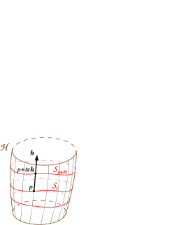
Figure 1: Foliation of a hypersurface ${\mathcal{H}}$ by a family $({\mathcal{S}}_{t})_{t\in\mathbb{R}}$ of spacelike 2-surfaces, and the associated evolution vector $\bm{h}$.

Demanding that the 2-surface ${\mathcal{S}}_{t}$ is spacelike amounts to saying that the metric $\bm{q}$ induced by the spacetime metric $\bm{g}$ onto ${\mathcal{S}}_{t}$ is positive definite (i.e. Riemannian). In particular $\bm{q}$ is not degenerate and at each point $p\in{\mathcal{S}}_{t}$, the following orthogonal decomposition holds:

$${\mathcal{T}}_{p}({\mathcal{M}})={\mathcal{T}}_{p}({\mathcal{S}}_{t})\oplus{\mathcal{T}}_{p}({\mathcal{S}}_{t})^{\perp},$$ (1)

where ${\mathcal{T}}_{p}({\mathcal{M}})$ [resp. ${\mathcal{T}}_{p}({\mathcal{S}}_{t})$] denotes the space of vectors tangent to ${\mathcal{M}}$ [resp. to ${\mathcal{S}}_{t}$] at the point $p$, and ${\mathcal{T}}_{p}({\mathcal{S}}_{t})^{\perp}$ denotes the space of vectors orthogonal to ${\mathcal{S}}_{t}$ at $p$. Both vector spaces ${\mathcal{T}}_{p}({\mathcal{S}}_{t})$ and ${\mathcal{T}}_{p}({\mathcal{S}}_{t})^{\perp}$ are two-dimensional. Let us then denote by $\bm{\vec{q}}$ the orthogonal projector onto ${\mathcal{T}}_{p}({\mathcal{S}}_{t})$: $\bm{\vec{q}}(\bm{v})=\bm{v}\iff\bm{v}\in{\mathcal{T}}_{p}({\mathcal{S}}_{t})$ and $\bm{\vec{q}}(\bm{v})=0\iff\bm{v}\in{\mathcal{T}}_{p}({\mathcal{S}}_{t})^{\perp}$. In this article, we shall take a 4-dimensional point of view on the induced metric $\bm{q}$ by setting $\bm{q}(\bm{u},\bm{v})=0$ if any of the two vectors $\bm{u}$ and $\bm{v}$ in ${\mathcal{T}}_{p}({\mathcal{M}})$ belongs to ${\mathcal{T}}_{p}({\mathcal{S}}_{t})^{\perp}$. Then, if in a given basis, the components of $\bm{q}$ are $q_{\alpha\beta}$, the components of $\vec{\bm{q}}$ are $q^{\alpha}_{\ \,\beta}$, where the index $\alpha$ has been raised with the metric $\bm{g}$.

Given a generic tensor $\bm{A}$ on ${\mathcal{T}}_{p}({\mathcal{M}})$ of covariance type $(m,n)$, we define a new tensor $\vec{\bm{q}}^{*}\bm{A}$ of the same covariance type thanks to the projector $\bm{\vec{q}}$:

$$\left(\vec{q}^{*}A\right)^{\alpha_{1}\ldots\alpha_{m}}_{\qquad\ \ \beta_{1}\ldots\beta_{n}} := q^{\alpha_{1}}_{\ \ \mu_{1}}\ldots q^{\alpha_{m}}_{\ \ \mu_{m}}q^{\nu_{1}}_{\ \ \beta_{1}}\ldots q^{\nu_{n}}_{\ \ \beta_{n}}\times$$ (2)

$$A^{\mu_{1}\ldots\mu_{m}}_{\qquad\ \ \nu_{1}\ldots\nu_{n}}.$$

Note that for a vector $\vec{\bm{q}}^{*}\bm{v}=\bm{\vec{q}}(\bm{v})$ and for a 1-form, $\vec{\bm{q}}^{*}\bm{\omega}=\bm{\omega}\circ\bm{\vec{q}}$. Note also that for multilinear forms intrinsic to the 2-dimensional manifold ${\mathcal{S}}_{t}$, $\vec{\bm{q}}^{*}$ can be viewed as the “push-forward” operator which transforms them to multilinear forms acting on the 4-dimensional space ${\mathcal{T}}_{p}({\mathcal{M}})$ (for vectors and more generally contravariant tensors, the push-forward operator is canonically provided by the embedding of ${\mathcal{S}}_{t}$ in ${\mathcal{M}}$). A tensor $\bm{A}$ on ${\mathcal{M}}$ will be said tangent to ${\mathcal{S}}_{t}$ if $\vec{\bm{q}}^{*}\bm{A}=\bm{A}$.

II.2 Evolution vector

Let us denote by $\bm{h}$ the vector field on ${\mathcal{H}}$ such that (see Fig. 1) (i) $\bm{h}$ is tangent to ${\mathcal{H}}$, (ii) at any point in ${\mathcal{H}}$, $\bm{h}$ is orthogonal to the surface ${\mathcal{S}}_{t}$ going through this point, (iii) the length of $\bm{h}$ is associated with the parameter $t$ labeling the surfaces $({\mathcal{S}}_{t})$ by

$$\bm{\mathcal{L}}_{\bm{h}}\,t=1,$$ (3)

where $\bm{\mathcal{L}}_{\bm{h}}\,$ denotes the Lie derivative along $\bm{h}$. In the present case (scalar field $t$), we have of course $\bm{\mathcal{L}}_{\bm{h}}\,t=h^{\mu}\partial_{\mu}t=\langle\bm{\mathrm{d}}t,\bm{h}\rangle$, where brackets are used to denote the action of 1-forms on vectors. Given the foliation $({\mathcal{S}}_{t})_{t\in\mathbb{R}}$, the conditions (i), (ii) and (iii) define $\bm{h}$ uniquely. Note however, that if the leaves ${\mathcal{S}}_{t}$ are relabeled by a new parameter $t^{\prime}=F(t)$ (where $F:\,\mathbb{R}\rightarrow\mathbb{R}$ is a smooth one-to-one map), then $\bm{h}$ is transformed into

$$\bm{h^{\prime}}=[F^{\prime}(t)]^{-1}\,\bm{h}$$ (4)

so that $\bm{\mathcal{L}}_{\bm{h^{\prime}}}\,t^{\prime}=1$.

An immediate consequence of Eq. (3) is that the 2-surfaces ${\mathcal{S}}_{t}$ are Lie-dragged by the vector field $\bm{h}$: given an infinitesimal parameter $\delta t$, the image of the surface ${\mathcal{S}}_{t}$ by the displacement of each of its points by the vector $\delta t\,\bm{h}$ is the surface ${\mathcal{S}}_{t+\delta t}$ (cf. Fig. 1). For this reason, $\bm{h}$ is the natural vector field to describe the “evolution” of quantities across the foliation of ${\mathcal{H}}$. In particular, we will consider the Lie derivative along $\bm{h}$, $\bm{\mathcal{L}}_{\bm{h}}\,$ as the “evolution operator” along ${\mathcal{H}}$. Since $\bm{h}$ Lie-drags the surfaces $({\mathcal{S}}_{t})$, it transports any vector tangent to ${\mathcal{S}}_{t}$ to a vector tangent to ${\mathcal{S}}_{t+\delta t}$. In other words,

$$\forall\bm{v}\in{\mathcal{T}}({\mathcal{S}}_{t}),\ \bm{\mathcal{L}}_{\bm{h}}\,\bm{v}\in{\mathcal{T}}({\mathcal{S}}_{t}),$$ (5)

where ${\mathcal{T}}({\mathcal{S}}_{t})$ denotes the space of vector fields defined on ${\mathcal{H}}$ and which are tangent to ${\mathcal{S}}_{t}$. Although the vector field $\bm{h}$ is not tangent to ${\mathcal{S}}_{t}$, we can use property (5) to extend the definition of $\bm{\mathcal{L}}_{\bm{h}}\,$ to 1-forms $\bm{\omega}$ acting in ${\mathcal{T}}({\mathcal{S}}_{t})$ (i.e. 2-dimensional 1-forms associated with the manifold structure of ${\mathcal{S}}_{t}$), by setting

$$\forall\bm{v}\in{\mathcal{T}}({\mathcal{S}}_{t}),\quad\langle\bm{\mathcal{L}}_{\bm{h}}\,\bm{\omega},\bm{v}\rangle:=\bm{\mathcal{L}}_{\bm{h}}\,\langle\bm{\omega},\bm{v}\rangle-\langle\bm{\omega},\bm{\mathcal{L}}_{\bm{h}}\,\bm{v}\rangle.$$ (6)

Note that the right-hand side of this equation is well defined thanks to Eq. (5). The definition of $\bm{\mathcal{L}}_{\bm{h}}\,$ is then extended immediately to any tensor field on ${\mathcal{S}}_{t}$ via tensor products and Leibniz’ rule, e.g. $\bm{\mathcal{L}}_{\bm{h}}\,(\bm{\omega}_{1}\otimes\bm{\omega}_{2}):=\bm{\mathcal{L}}_{\bm{h}}\,\bm{\omega}_{1}\otimes\bm{\omega}_{2}+\bm{\omega}_{1}\otimes\bm{\mathcal{L}}_{\bm{h}}\,\bm{\omega}_{2}$. Given a multilinear form field $\bm{A}$ on ${\mathcal{S}}_{t}$, we then denote by ${}^{{\mathcal{S}}}\!\bm{\mathcal{L}}_{\bm{h}}\,\bm{A}$ the push-forward (via the projector $\bm{\vec{q}}$) of the derivative $\bm{\mathcal{L}}_{\bm{h}}\,\bm{A}$ defined above:

$${}^{{\mathcal{S}}}\!\bm{\mathcal{L}}_{\bm{h}}\,\bm{A}:=\vec{\bm{q}}^{*}\bm{\mathcal{L}}_{\bm{h}}\,\bm{A}.$$ (7)

One can then show that (see Appendix A of Ref. GourgJ05 for details):

$${}^{{\mathcal{S}}}\!\bm{\mathcal{L}}_{\bm{h}}\,\bm{A}=\vec{\bm{q}}^{*}\bm{\mathcal{L}}_{\bm{h}}\,\vec{\bm{q}}^{*}\bm{A},$$ (8)

where the Lie derivative in the right-hand side is the standard Lie derivative along $\bm{h}$ within the manifold ${\mathcal{M}}$.

Owing to the fundamental property (3) and the resulting Lie-dragging of the surfaces $({\mathcal{S}}_{t})$, it is not surprising that the vector $\bm{h}$ has been introduced by many authors when studying foliation of hypersurfaces, in various contexts: $\bm{h}$ and $\bm{\mathcal{L}}_{\bm{h}}\,$ were denoted respectively $\bm{\ell}$ and $D/dt$ by Damour Damou78 ; Damou79 ; Damou82 in his black hole mechanics (${\mathcal{H}}$ was then taken to be an event horizon); $\bm{h}$ was denoted $\partial^{(n)}_{t}$ by Eardley Eardl98 in his study of black hole boundary conditions for 3+1 numerical relativity, since it was then viewed as the part of the evolution vector ${\partial/\partial t}$ which is normal to ${\mathcal{S}}_{t}$ in a coordinate system adapted to ${\mathcal{H}}$. Similarly, $\bm{h}$ is denoted $\vec{\zeta}$ by Cook Cook02 when searching for boundary conditions for initial data representing quasi-stationary black holes. More recently, in the context of trapping and dynamical horizons, $\bm{h}$ has been denoted $\overline{V}^{a}$ by Ashtekar and Krishnan AshteK03 , $\bm{\mathcal{V}}$ by Booth and Fairhurst BoothF04 ; BoothF05 and $\bm{\xi}$ by Hayward Haywa04c ; Haywa04b .

Let $C$ be the scalar field defined on ${\mathcal{H}}$ as half the scalar square of $\bm{h}$:

$$C:=\frac{1}{2}\,\bm{h}\cdot\bm{h},$$ (9)

where a dot is used to denote the scalar product taken with the metric $\bm{g}$. Since $\bm{h}$ is normal to ${\mathcal{S}}_{t}$, an orthogonal vector basis of ${\mathcal{T}}_{p}({\mathcal{H}})$ is $(\bm{h},\bm{e}_{2},\bm{e}_{3})$, where $(\bm{e}_{2},\bm{e}_{3})$ is an orthonormal basis of ${\mathcal{T}}_{p}({\mathcal{S}}_{t})$. In this basis, the matrix of the metric induced by $\bm{g}$ on ${\mathcal{H}}$ is $\mathrm{diag}(2C,1,1)$. We then conclude that

$$\begin{array}[]{lclcl}{\mathcal{H}}\ \mbox{is spacelike}&\iff&C>0&\iff&\bm{h}\ \mbox{is spacelike}\\ {\mathcal{H}}\ \mbox{is null}&\iff&C=0&\iff&\bm{h}\ \mbox{is null}\\ {\mathcal{H}}\ \mbox{is timelike}&\iff&C<0&\iff&\bm{h}\ \mbox{is timelike.}\end{array}$$ (10)

III Extrinsic geometry of a spacelike 2-surface

In this section, we review some basic results about the extrinsic geometry of a single spacelike 2-surface — not necessarily a member of a foliation. For future purpose, we take care to provide rather general definitions, for instance not limiting the definition of expansion and shear to null vectors, as usually done, nor limiting the definition of the normal fundamental forms to some privileged normal frame.

III.1 Expansion and shear along normal vectors

Let us consider a fixed 2-surface ${\mathcal{S}}_{t}$. We denote by ${\mathcal{T}}({\mathcal{S}}_{t})^{\perp}$ the space of vector fields $\bm{v}$ which are defined on ${\mathcal{S}}_{t}$ and everywhere normal to ${\mathcal{S}}_{t}$: $\forall p\in{\mathcal{S}}_{t},\ \bm{v}(p)\in{\mathcal{T}}_{p}({\mathcal{S}}_{t})^{\perp}$. For any $\bm{v}\in{\mathcal{T}}({\mathcal{S}}_{t})^{\perp}$, we define the deformation tensor of ${\mathcal{S}}_{t}$ along $\bm{v}$ as the bilinear form

$$\bm{\Theta}^{(\bm{v})}:=\vec{\bm{q}}^{*}\bm{\nabla}\underline{\bm{v}}\quad\left[\mbox{or}\ \Theta^{(\bm{v})}_{\alpha\beta}:=\nabla_{\nu}v_{\mu}\,q^{\mu}_{\ \,\alpha}q^{\nu}_{\ \,\beta}\right],$$ (11)

where $\bm{\nabla}$ is the affine connection associated with the spacetime metric $\bm{g}$ and the underlining is used to denote in an index-free way the 1-form $\underline{\bm{v}}$ canonically associated to the vector field $\bm{v}$ by the metric $\bm{g}$. Note that thanks to the projector $\bm{\vec{q}}$ in Eq. (11), $\bm{\Theta}^{(\bm{v})}$ is independent of the values of $\bm{v}$ away from ${\mathcal{S}}_{t}$ (some extension of $\bm{v}$ in an open neighborhood of ${\mathcal{S}}_{t}$ being required for the spacetime covariant derivative $\bm{\nabla}\underline{\bm{v}}$ to be well defined). It is easy to see that the bilinear form $\bm{\Theta}^{(\bm{v})}$ is symmetric, as the consequence of $\bm{v}$ being normal to the surface ${\mathcal{S}}_{t}$ (Weingarten property).

Let us consider the metric $\bm{\tilde{q}}$ induced by $\bm{g}$ on the 2-surfaces deduced from ${\mathcal{S}}_{t}$ by Lie-dragging along $\bm{v}$ (recall that $\bm{q}$ is a priori defined only on ${\mathcal{S}}_{t}$; we have of course $\bm{\tilde{q}}\stackrel{{\scriptstyle{\mathcal{S}}_{t}}}{{=}}\bm{q}$). Taking into account the symmetry of $\bm{\Theta}^{(\bm{v})}$ and expressing the Lie derivative in terms of $\bm{\nabla}$ yields $\vec{\bm{q}}^{*}\bm{\mathcal{L}}_{\bm{v}}\,\bm{\tilde{q}}=\vec{\bm{q}}^{*}\bm{\nabla}_{\bm{v}}\bm{\tilde{q}}+2\bm{\Theta}^{(\bm{v})}$. Now, from the idempotent character of $\bm{\vec{q}}$, it is easy to see that $\vec{\bm{q}}^{*}\bm{\nabla}_{\bm{v}}\bm{\tilde{q}}=0$, so that finally one ends with

$$\bm{\Theta}^{(\bm{v})}=\frac{1}{2}\,\vec{\bm{q}}^{*}\bm{\mathcal{L}}_{\bm{v}}\,\bm{\tilde{q}}.$$ (12)

This equality justifies the name deformation tensor given to $\bm{\Theta}^{(\bm{v})}$: $\bm{\Theta}^{(\bm{v})}$ measures the variation of the metric in ${\mathcal{S}}_{t}$ when this surface is Lie-dragged along the vector $\bm{v}$. Decomposing $\bm{\Theta}^{(\bm{v})}$ into a trace part and a traceless part results in the definition of the expansion rate of ${\mathcal{S}}_{t}$ along $\bm{v}$:

$$\theta^{(\bm{v})}:=q^{\mu\nu}\Theta^{(\bm{v})}_{\mu\nu}=\bm{\mathcal{L}}_{\bm{v}}\,\ln\sqrt{\tilde{q}},$$ (13)

and the shear tensor of ${\mathcal{S}}_{t}$ along $\bm{v}$:

$$\bm{\sigma}^{(\bm{v})}:=\bm{\Theta}^{(\bm{v})}-\frac{1}{2}\,\theta^{(\bm{v})}\,\bm{q}.$$ (14)

In Eq. (13) the second equality results from Eq. (12), $\tilde{q}$ being the determinant of the components $\tilde{q}_{ab}$ with respect to a coordinate system $x^{a}=(x^{2},x^{3})$ of the induced metric on the surface obtained from ${\mathcal{S}}_{t}$ by Lie-drag along $\bm{v}$. Since $\sqrt{q}$ is related to the surface element ${}^{\scriptscriptstyle\mathcal{S}}\!\bm{\epsilon}$ of ${\mathcal{S}}_{t}$ by ${}^{\scriptscriptstyle\mathcal{S}}\!\bm{\epsilon}=\sqrt{q}\,\bm{\mathrm{d}}x^{2}\wedge\bm{\mathrm{d}}x^{3}$, we see by considering coordinates $x^{a}$ constant along $\bm{v}$ field lines that $\theta^{(\bm{v})}$ is nothing but the relative rate of change of the area of a surface element Lie-dragged by $\bm{v}$ from ${\mathcal{S}}_{t}$:

$$\bm{\mathcal{L}}_{\bm{\bm{v}}}\,{}^{\scriptscriptstyle\mathcal{S}}\!\bm{\epsilon}=\theta^{(\bm{v})}\,{}^{\scriptscriptstyle\mathcal{S}}\!\bm{\epsilon},$$ (15)

hence the name expansion rate given to $\theta^{(\bm{v})}$.

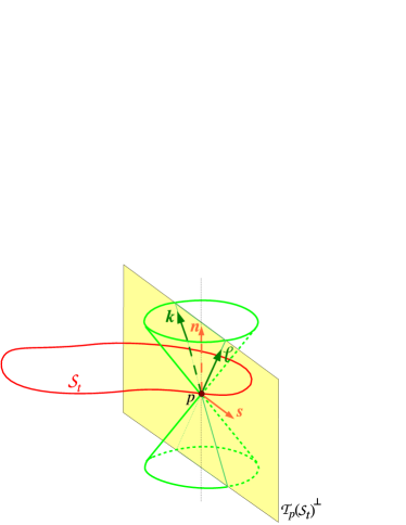
Figure 2: Vector plane ${\mathcal{T}}_{p}({\mathcal{S}}_{t})^{\perp}$ normal to ${\mathcal{S}}_{t}$ at a given point $p$, with some orthonormal frame $(\bm{n},\bm{s})$ and some null frame $(\bm{\ell},\bm{k})$. The directions of $\bm{\ell}$ and $\bm{k}$ are uniquely defined as the intersections of ${\mathcal{T}}_{p}({\mathcal{S}}_{t})^{\perp}$ with the light cone emanating from $p$, whereas the directions of $\bm{n}$ and $\bm{s}$ can be changed by an arbitrary boost in a direction normal to ${\mathcal{S}}_{t}$.

III.2 Normal frames

From the decomposition (1) and the spacelike character of ${\mathcal{S}}_{t}$, we see that the restriction of the metric $\bm{g}$ to the vector plane ${\mathcal{T}}_{p}({\mathcal{S}}_{t})^{\perp}$ orthogonal to ${\mathcal{S}}_{t}$ must be of signature $(-,+)$. There are then two natural choices of pairs of vectors for generating this plane: (i) an orthonormal basis $(\bm{n},\bm{s})$, i.e. a timelike vector $\bm{n}$ and a spacelike vector $\bm{s}$ satisfying

$$\bm{n}\cdot\bm{n}=-1,\quad\bm{s}\cdot\bm{s}=1,\quad\bm{n}\cdot\bm{s}=0;$$ (16)

(ii) a pair of linearly independent future-directed null vectors $(\bm{\ell},\bm{k})$; this choice is permissible since the signature $(-,+)$ implies that ${\mathcal{T}}_{p}({\mathcal{S}}_{t})^{\perp}$ contains two null directions, which are actually the intersections of the null cone emanating from $p$ with ${\mathcal{T}}_{p}({\mathcal{S}}_{t})^{\perp}$ (cf. Fig. 2):

$$\bm{\ell}\cdot\bm{\ell}=0,\quad\bm{k}\cdot\bm{k}=0,\quad\bm{\ell}\cdot\bm{k}=:-e^{\sigma},$$ (17)

where $\bm{\ell}\cdot\bm{k}$ is negative (hence written as minus some exponential) as a result of both $\bm{\ell}$ and $\bm{k}$ being future-directed.

In both cases, there is not a unique choice: in case (i), the timelike and spacelike directions can be changed by a boost in an arbitrary direction normal to ${\mathcal{S}}_{t}$, leading to a new pair of basis vectors:

$$\bm{n^{\prime}} = \cosh\eta\,\bm{n}+\sinh\eta\,\bm{s}$$ (18)

$$\bm{s^{\prime}} = \sinh\eta\,\bm{n}+\cosh\eta\,\bm{s},$$ (19)

where $\eta\in\mathbb{R}$ is the boost parameter. The choice $(\bm{n},\bm{s})$ can be made unique by invoking some extra structure like the global foliation $(\Sigma_{t})_{t\in\mathbb{R}}$ of ${\mathcal{M}}$ arising from the 3+1 perspective mentioned in Sec. 1, $\bm{n}$ being then the future directed unit normal to $\Sigma_{t}$ and $\bm{s}$ one of the two unit normals to ${\mathcal{S}}_{t}$ which are tangent to $\Sigma_{t}$. Another definite choice of $(\bm{n},\bm{s})$ can be performed when ${\mathcal{H}}$ is spacelike (resp. timelike), by demanding that $\bm{n}$ (resp. $\bm{s}$) is normal to ${\mathcal{H}}$; $\bm{s}$ (resp. $\bm{n}$) is then colinear to the evolution vector $\bm{h}$, and in particular lies in ${\mathcal{H}}$. This is the choice adopted by Ashtekar and Krishnan AshteK02 ; AshteK03 ; AshteK04 for dynamical horizons, which are always spacelike (see Appendix A).

In case (ii), the two null directions are unique, but the vectors $\bm{\ell}$ and $\bm{k}$ can be rescaled arbitrarily by

$$\bm{\ell^{\prime}} = \lambda\,\bm{\ell},\qquad\lambda>0$$ (20)

$$\bm{k^{\prime}} = \mu\,\bm{k},\qquad\mu>0,$$ (21)

where the positive sign of $\lambda$ and $\mu$ is chosen to preserve the future orientation. One may reduce the arbitrariness by fixing the scalar product $\bm{\ell}\cdot\bm{k}$ to $-1$ [choice $\sigma=0$ in Eq. (17)], but this determines only $\mu$ as being $\lambda^{-1}$ and leaves the degree of freedom on $\lambda$. We will see in Sec. IV.2 that, when considering not a single ${\mathcal{S}}_{t}$, but the whole foliation $({\mathcal{S}}_{t})_{t\in\mathbb{R}}$, this ambiguity can be fixed in a natural way, leading to a unique choice of $(\bm{\ell},\bm{k})$.

Note that for the choice (i), the orthogonal projector $\bm{\vec{q}}$ on ${\mathcal{S}}_{t}$ is expressible as

$$\bm{\vec{q}}=\bm{1}+\langle\underline{\bm{n}},.\rangle\,\bm{n}-\langle\underline{\bm{s}},.\rangle\,\bm{s}$$ (22)

(equivalently $\bm{q}=\bm{g}+\underline{\bm{n}}\otimes\underline{\bm{n}}-\underline{\bm{s}}\otimes\underline{\bm{s}}$), whereas for the choice (ii)

$$\bm{\vec{q}}=\bm{1}+e^{-\sigma}\langle\underline{\bm{k}},.\rangle\,\bm{\ell}+e^{-\sigma}\langle\underline{\bm{\ell}},.\rangle\,\bm{k}$$ (23)

(equivalently $\bm{q}=\bm{g}+e^{-\sigma}\,\underline{\bm{k}}\otimes\underline{\bm{\ell}}+e^{-\sigma}\,\underline{\bm{\ell}}\otimes\underline{\bm{k}}$).

${\mathcal{S}}_{t}$ is called a trapped surface if, in addition of being spacelike and closed, it satisfies $\theta^{(\bm{\ell})}<0$ and $\theta^{(\bm{k})}<0$, and a marginally trapped surface if $\theta^{(\bm{\ell})}=0$ and $\theta^{(\bm{k})}<0$, or $\theta^{(\bm{\ell})}<0$ and $\theta^{(\bm{k})}=0$ Penro65 . If one of the two null directions, $\bm{\ell}$ say, can be selected as being “outgoing”, ${\mathcal{S}}_{t}$ is called an outer trapped surface if $\theta^{(\bm{\ell})}<0$ (irrespectively of the sign of $\theta^{(\bm{k})}$) HawkiE73 . It is called a marginally outer trapped surface (MOTS) if $\theta^{(\bm{\ell})}=0$. Notice that all these definitions are unaffected by the rescaling (20)-(21) of the null vectors $\bm{\ell}$ and $\bm{k}$.

III.3 Second fundamental tensor

As for any non-null submanifold of $({\mathcal{M}},\bm{g})$, the second fundamental tensor of ${\mathcal{S}}_{t}$ (also called extrinsic imbedding curvature tensor Carte92a or shape tensor Senov04 ) is defined as the tensor $\bm{\mathcal{K}}$ of type $(1,2)$ relating the covariant derivative of a vector tangent to ${\mathcal{S}}_{t}$ taken with the spacetime connection $\bm{\nabla}$ to that taken with the connection in ${\mathcal{S}}_{t}$ compatible with the induced metric $\bm{q}$, hereafter denoted by $\bm{\mathcal{D}}$:

$$\forall(\bm{u},\bm{v})\in{\mathcal{T}}({\mathcal{S}}_{t})^{2},\quad\bm{\nabla}_{\bm{u}}\bm{v}=\bm{\mathcal{D}}_{\bm{u}}\bm{v}+\bm{\mathcal{K}}(\bm{u},\bm{v}).$$ (24)

From the fundamental relation

$$\bm{\mathcal{D}}\bm{A}=\vec{\bm{q}}^{*}\bm{\nabla}\bm{A},$$ (25)

valid for any tensorial field $\bm{A}$ tangent to ${\mathcal{S}}_{t}$, it is easy to express $\bm{\mathcal{K}}$ in terms of the derivative of $\bm{\vec{q}}$:

$$\mathcal{K}^{\alpha}_{\ \,\beta\gamma}=\nabla_{\mu}q^{\alpha}_{\ \,\nu}\;q^{\mu}_{\ \,\beta}q^{\nu}_{\ \,\gamma}.$$ (26)

Let $(\bm{n},\bm{s})$ be an orthonormal frame of ${\mathcal{T}}({\mathcal{S}}_{t})^{\perp}$; inserting expression (22) for $q^{\alpha}_{\ \,\nu}$ in the above relation and making use of definition (11) leads to

$$\mathcal{K}^{\alpha}_{\ \,\beta\gamma}=n^{\alpha}\,\Theta^{(\bm{n})}_{\beta\gamma}-s^{\alpha}\,\Theta^{(\bm{s})}_{\beta\gamma}.$$ (27)

Similarly, if one uses instead a null frame $(\bm{\ell},\bm{k})$ for ${\mathcal{T}}({\mathcal{S}}_{t})^{\perp}$, expression (23) for $q^{\alpha}_{\ \,\nu}$ leads to

$$\mathcal{K}^{\alpha}_{\ \,\beta\gamma}=e^{-\sigma}\left(k^{\alpha}\,\Theta^{(\bm{\ell})}_{\beta\gamma}+\ell^{\alpha}\,\Theta^{(\bm{k})}_{\beta\gamma}\right).$$ (28)

It is clear on formulas (27) and (28) that the second fundamental tensor is orthogonal to ${\mathcal{S}}_{t}$ in its first index, and symmetric and tangent to ${\mathcal{S}}_{t}$ in its second and third indices. The reader more familiar with the hypersurface case should note that the second fundamental tensor for a hypersurface writes, instead of Eq. (27), $\mathcal{K}^{\alpha}_{\ \,\beta\gamma}=-n^{\alpha}K_{\beta\gamma}$, where $n^{\alpha}$ is the normal to the hypersurface and $K_{\beta\gamma}$ its second fundamental form or extrinsic curvature tensor.

III.4 Normal fundamental forms

Contrary to the case of a hypersurface, the extrinsic geometry of the 2-surface ${\mathcal{S}}_{t}$ is not entirely specified by the second fundamental tensor $\bm{\mathcal{K}}$. Indeed, because it involves only the deformation tensors $\bm{\Theta}^{(.)}$ of the normals to ${\mathcal{S}}_{t}$ [cf. Eqs. (27) and (28)], $\bm{\mathcal{K}}$ encodes only the part of the variation of ${\mathcal{S}}_{t}$’s normals which is parallel to ${\mathcal{S}}_{t}$. It does not encode the variation of the two normals with respect to each other. The latter is devoted to the normal fundamental forms which are the 1-forms defined by (cf. e.g. Haywa94b or Epp00 )

$$\bm{\Omega}^{(\bm{n})} := \bm{s}\cdot\bm{\nabla}_{\bm{\vec{q}}}\,\bm{n}\quad\left[\mbox{or}\ \Omega^{(\bm{n})}_{\alpha}:=s_{\mu}\nabla_{\nu}n^{\mu}\,q^{\nu}_{\ \,\alpha}\right]$$ (29)

$$\bm{\Omega}^{(\bm{s})} := \bm{n}\cdot\bm{\nabla}_{\bm{\vec{q}}}\,\bm{s}\quad\left[\mbox{or}\ \Omega^{(\bm{s})}_{\alpha}:=n_{\mu}\nabla_{\nu}s^{\mu}\,q^{\nu}_{\ \,\alpha}\right]$$ (30)

if one considers an orthonormal frame $(\bm{n},\bm{s})$ of ${\mathcal{T}}({\mathcal{S}}_{t})^{\perp}$ and by

$$\bm{\Omega}^{(\bm{\ell})}:=\frac{1}{\bm{k}\cdot\bm{\ell}}\,\bm{k}\cdot\bm{\nabla}_{\bm{\vec{q}}}\,\bm{\ell}\quad\left[\mbox{or}\ \Omega^{(\bm{\ell})}_{\alpha}:=\frac{1}{k_{\rho}\ell^{\rho}}k_{\mu}\nabla_{\nu}\ell^{\mu}\,q^{\nu}_{\ \,\alpha}\right]$$ (31)

$$\bm{\Omega}^{(\bm{k})}:=\frac{1}{\bm{k}\cdot\bm{\ell}}\,\bm{\ell}\cdot\bm{\nabla}_{\bm{\vec{q}}}\,\bm{k}\quad\left[\mbox{or}\ \Omega^{(\bm{k})}_{\alpha}:=\frac{1}{k_{\rho}\ell^{\rho}}\ell_{\mu}\nabla_{\nu}k^{\mu}\,q^{\nu}_{\ \,\alpha}\right]$$ (32)

if a null frame $(\bm{\ell},\bm{k})$ of ${\mathcal{T}}({\mathcal{S}}_{t})^{\perp}$ is considered instead. Note that, thanks to the projector $\bm{\vec{q}}$, the definition of the normal fundamental forms does not depend upon the values of the normal fields $\bm{n}$, $\bm{s}$, $\bm{\ell}$ and $\bm{k}$ away from the 2-surface ${\mathcal{S}}_{t}$. Note also that thanks to the division by $\bm{k}\cdot\bm{\ell}$, the value of $\bm{\Omega}^{(\bm{\ell})}$ does not depend on the choice of the null vector $\bm{k}$ complementary to $\bm{\bm{\ell}}$. From the orthogonality relations (16) and (17), we have the immediate properties:

$$\bm{\Omega}^{(\bm{s})} = -\bm{\Omega}^{(\bm{n})}$$ (33)

$$\bm{\Omega}^{(\bm{k})} = -\bm{\Omega}^{(\bm{\ell})}+\bm{\mathcal{D}}\sigma.$$ (34)

We can also relate the $(\bm{\ell},\bm{k})$-type normal fundamental forms to the $(\bm{n},\bm{s})$-type ones by choosing the canonical null frame associated with a given orthonormal frame $(\bm{n},\bm{s})$, namely $\bm{\ell}=\bm{n}+\bm{s}$ and $\bm{k}=\bm{n}-\bm{s}$. Then

$$\bm{\Omega}^{(\bm{\ell})} = \bm{\Omega}^{(\bm{n})}\qquad[\bm{\ell}=\bm{n}+\bm{s}]$$ (35)

$$\bm{\Omega}^{(\bm{k})} = -\bm{\Omega}^{(\bm{n})}\qquad[\bm{k}=\bm{n}-\bm{s}].$$ (36)

Note that, if one considers a non-null hypersurface instead of a 2-surface, the analog of definition (29) would be $\bm{\Omega}^{(\bm{n})}:=\bm{n}\cdot\bm{\nabla}_{\bm{\vec{q}}}\,\bm{n}$, since there is only one normal $\bm{n}$. But this expression vanishes identically by virtue of the normalization of $\bm{n}$ ($\bm{n}\cdot\bm{n}=1$ for a timelike hypersurface, and $-1$ for a spacelike one). Consequently, the extrinsic curvature of a non-null hypersurface is entirely characterized by the second fundamental form $\bm{K}$. For a null hypersurface, with normal $\bm{\ell}$, the orthogonal projector $\bm{\vec{q}}$ is not defined (as a result of $\bm{q}$ being degenerate). The relevant quantity is then the 1-form $\bm{\Omega}^{(\bm{\ell})}$ defined by Eq. (31) but with $\bm{\vec{q}}$ substituted with the orthogonal projector to some spacelike 2-surface embedded in the hypersurface and $\bm{k}$ substituted with a transverse null vector. It is then called the Háj́iček  1-form Hajic73 ; Hajic75 (see also GourgJ05 ).

The normal fundamental forms can be interpreted in terms of the connection 1-forms associated with respect to some tetrad. Indeed let $\bm{e}_{\alpha}=(\bm{n},\bm{s},\bm{e}_{2},\bm{e}_{3})$ be an orthonormal tetrad [$(\bm{e}_{2},\bm{e}_{3})$ is then an orthonormal basis of ${\mathcal{T}}_{p}({\mathcal{S}}_{t})$]. The connection 1-forms associated with this tetrad are the 1-forms $\bm{\omega}^{\beta}_{\ \,\alpha}$ such that for any vector field $\bm{v}$ on ${\mathcal{M}}$, $\bm{\nabla}_{\bm{v}}\,\bm{e}_{\alpha}=\langle\bm{\omega}^{\mu}_{\ \,\alpha},\bm{v}\rangle\,\bm{e}_{\mu}$. Then, from Eq. (29),

$$\bm{\Omega}^{(\bm{n})}=\vec{\bm{q}}^{*}\bm{\omega}^{1}_{\ \,0}.$$ (37)

An equivalent phrasing of this is saying that the two non-trivial components of $\bm{\Omega}^{(\bm{n})}$ with respect to the dual frame $(\bm{e}^{\alpha})$, namely $\Omega^{(\bm{n})}_{a}$ ($a=2,3$), are identical to some of the connection coefficients $\Gamma^{\alpha}_{\ \,\beta\gamma}$ associated with the tetrad $(\bm{e}_{\alpha})$:

$$\Omega^{(\bm{n})}_{a}=\Gamma^{1}_{\ \,0a}.$$ (38)

Relations (37) and (38) justify the alternative names external rotation coefficients Carte92a and connection on the normal bundle Epp00 ; BoothF05 ; Szaba04 given to the normal fundamental forms.

The normal fundamental forms depend on the normal frame. Indeed a change of normal frame $(\bm{n},\bm{s})\mapsto(\bm{n^{\prime}},\bm{s^{\prime}})$ according to Eqs. (18)-(19) leads to

$$\bm{\Omega}^{(\bm{n^{\prime}})}=\bm{\Omega}^{(\bm{n})}+\bm{\mathcal{D}}\eta,$$ (39)

whereas a change of null normal frame $(\bm{\ell},\bm{k})\mapsto(\bm{\ell^{\prime}},\bm{k^{\prime}})$ according to Eqs. (20)-(21) leads to

$$\bm{\Omega}^{(\bm{\ell^{\prime}})}=\bm{\Omega}^{(\bm{\ell})}+\bm{\mathcal{D}}\ln\lambda.$$ (40)

On the contrary, the second fundamental tensor $\bm{\mathcal{K}}$ introduced in the previous section does not depend on the choice of the normal frame: this is obvious from Eq. (26) which involves only the projector $\bm{\vec{q}}$, and this can be checked easily from the expressions in term of the normal frames [Eqs. (27) and (28)], by substituting the transformation laws (18)-(19) and (20)-(21). We refer the reader to Carter’s article Carte92a for an extended discussion of this dependence of the normal fundamental forms with respect to the normal frames.

IV Extrinsic geometry of the foliation

Section III introduced quantities relative to a single 2-surface ${\mathcal{S}}_{t}$. Here we investigate quantities defined with respect to the family $({\mathcal{S}}_{t})_{t\in\mathbb{R}}$ foliating ${\mathcal{H}}$.

IV.1 Dual-null description of the foliation $({\mathcal{S}}_{t})_{t\in\mathbb{R}}$

A very convenient way to study the foliation $({\mathcal{S}}_{t})_{t\in\mathbb{R}}$ is to employ of the dual-null formalism of Hayward Haywa93 ; Haywa94b ; Haywa01 (see also InverS80 ; BradyDIM96 ), which we recall here, adapting the notations to our purpose (see Table 1 for the correspondence with Hayward’s notations).

Let us consider, in the neighborhood of ${\mathcal{H}}$, two families of null hypersurfaces, $(\mathcal{U}_{u})_{u\in\mathbb{R}}$ and $(\mathcal{V}_{v})_{v\in\mathbb{R}}$, which intersect in spatial 2-surfaces such that each 2-surface ${\mathcal{S}}_{t}$ is one of these intersections, i.e. for each $t\in\mathbb{R}$, there exists a value of $u$, $u_{0}(t)$ say, and a value of $v$, $v_{0}(t)$ say, such that ${\mathcal{S}}_{t}$ is the intersection between $\mathcal{U}_{u_{0}(t)}$ and $\mathcal{V}_{v_{0}(t)}$:

$$\forall t\in\mathbb{R},\quad{\mathcal{S}}_{t}=\mathcal{U}_{u_{0}(t)}\cap\mathcal{V}_{v_{0}(t)}.$$ (41)

Such a dual-null foliation always exists, $\mathcal{U}_{u_{0}(t)}$ (resp. $\mathcal{V}_{v_{0}(t)}$) being nothing but the hypersurface generated by light rays outgoing (resp. ingoing) orthogonally from ${\mathcal{S}}_{t}$. Moreover, if ${\mathcal{H}}$ is spacelike or timelike, the dual-null foliation is unique. If ${\mathcal{H}}$ is null, then ${\mathcal{H}}$ coincides with $\mathcal{U}_{u_{0}(t)}$ and $u_{0}(t)=\mathrm{const}.$; there is then the degree of freedom of choosing the foliation $(\mathcal{U}_{u})$ outside of ${\mathcal{H}}$.

Let $\bm{\tilde{\ell}}$ and $\bm{\tilde{k}}$ be the null normal vectors to respectively $\mathcal{U}_{u}$ and $\mathcal{V}_{v}$ and dual (up to a sign) to the gradient 1-forms $\bm{\mathrm{d}}u$ and $\bm{\mathrm{d}}v$:

$$\underline{\bm{\tilde{\ell}}}:=-\bm{\mathrm{d}}u\qquad\mbox{and}\qquad\underline{\bm{\tilde{k}}}:=-\bm{\mathrm{d}}v.$$ (42)

Since ${\mathcal{S}}_{t}$ belongs to both $\mathcal{U}_{u_{0}(t)}$ and $\mathcal{V}_{v_{0}(t)}$, both $\bm{\tilde{\ell}}$ and $\bm{\tilde{k}}$ are normal to ${\mathcal{S}}_{t}$, and therefore constitute a null frame of ${\mathcal{T}}({\mathcal{S}}_{t})^{\perp}$, similar to those considered in Sec. III.2. Let us denote $f$ the scalar field $\sigma$ associated to the scalar product of $\bm{\tilde{\ell}}$ and $\bm{\tilde{k}}$ by Eq. (17):

$$\bm{\tilde{\ell}}\cdot\bm{\tilde{k}}=:-e^{f}.$$ (43)

From the definition (42), the 1-forms $\underline{\bm{\tilde{\ell}}}$ and $\underline{\bm{\tilde{k}}}$ are closed:

$$\bm{\mathrm{d}}\underline{\bm{\tilde{\ell}}}=0\qquad\mbox{and}\qquad\bm{\mathrm{d}}\underline{\bm{\tilde{k}}}=0.$$ (44)

The vectors $\bm{\tilde{\ell}}$ and $\bm{\tilde{k}}$ being null, it follows immediately from Eq. (44) that

$$\bm{\nabla}_{\bm{\tilde{\ell}}}\,\bm{\tilde{\ell}}=0\qquad\mbox{and}\qquad\bm{\nabla}_{\bm{\tilde{k}}}\,\bm{\tilde{k}}=0,$$ (45)

i.e. the field lines of $\bm{\tilde{\ell}}$ and $\bm{\tilde{k}}$ are geodesics: they are the light rays emanating orthogonally from ${\mathcal{S}}_{t}$. Hayward Haywa93 ; Haywa94b ; Haywa01 ; Haywa04c ; Haywa04b introduces another pair of null vectors by setting

$$\bm{\hat{\ell}}:=e^{-f}\bm{\tilde{\ell}}\qquad\mbox{and}\qquad\bm{\hat{k}}:=e^{-f}\bm{\tilde{k}}.$$ (46)

These vectors have the fundamental property of Lie-dragging the hypersurfaces $\mathcal{V}_{v}$ and $\mathcal{U}_{u}$ respectively, i.e. they obey

$$\bm{\mathcal{L}}_{\bm{\bm{\hat{\ell}}}}\,v=1\qquad\mbox{and}\qquad\bm{\mathcal{L}}_{\bm{\bm{\hat{k}}}}\,u=1,$$ (47)

but contrary to $\underline{\bm{\tilde{\ell}}}$ and $\underline{\bm{\tilde{k}}}$, the 1-forms $\underline{\bm{\hat{\ell}}}$ and $\underline{\bm{\hat{k}}}$ are not closed, since we deduce from Eq. (44) that

$$\bm{\mathrm{d}}\underline{\bm{\hat{\ell}}}=-\bm{\mathrm{d}}f\wedge\underline{\bm{\hat{\ell}}}\qquad\mbox{and}\qquad\bm{\mathrm{d}}\underline{\bm{\hat{k}}}=-\bm{\mathrm{d}}f\wedge\underline{\bm{\hat{k}}}.$$ (48)

Besides,

$$\bm{\hat{\ell}}\cdot\bm{\hat{k}}=-e^{-f}.$$ (49)

The anholonomicity 1-form, also called twist 1-form, is defined by [cf. Appendix B of Ref. Haywa94b , in conjunction with our definitions (31) and (32)]:

$$\bm{\varpi}:=\frac{1}{2}\left(\bm{\Omega}^{(\bm{\tilde{k}})}-\bm{\Omega}^{(\bm{\tilde{\ell}})}\right).$$ (50)

From Eq. (34) with $\sigma=f$, we get

$$\bm{\varpi}=-\bm{\Omega}^{(\bm{\tilde{\ell}})}+\frac{1}{2}\bm{\mathcal{D}}f=\bm{\Omega}^{(\bm{\tilde{k}})}-\frac{1}{2}\bm{\mathcal{D}}f.$$ (51)

According to the scaling law (40) with $\lambda=e^{-f}$ [cf. Eq. (46)], we can re-express the anholonomicity 1-form in terms of the normal fundamental forms associated with $\bm{\hat{\ell}}$ and $\bm{\hat{k}}$:

$$\bm{\varpi}=-\bm{\Omega}^{(\bm{\hat{\ell}})}-\frac{1}{2}\bm{\mathcal{D}}f=\bm{\Omega}^{(\bm{\hat{k}})}+\frac{1}{2}\bm{\mathcal{D}}f.$$ (52)

Thanks to Eq. (44), we can easily re-express $\bm{\varpi}$ in term of the commutator of $\bm{\tilde{k}}$ and $\bm{\tilde{\ell}}$, as well as that of $\bm{\hat{k}}$ and $\bm{\hat{\ell}}$:

$$\bm{\varpi}=\frac{e^{-f}}{2}\,\bm{q}\cdot[\bm{\tilde{k}},\bm{\tilde{\ell}}]=\frac{e^{f}}{2}\,\bm{q}\cdot[\bm{\hat{k}},\bm{\hat{\ell}}]$$ (53)

$$\left[\mbox{or}\quad\varpi_{\alpha}=\frac{e^{-f}}{2}\,q_{\alpha\mu}[\tilde{k},\tilde{\ell}]^{\mu}=\frac{e^{f}}{2}\,q_{\alpha\mu}[\hat{k},\hat{\ell}]^{\mu}\right].$$ (54)

This justifies the terms anholonomicity and twist given to $\bm{\varpi}$: according to Frobenius theorem, the 2-planes ${\mathcal{T}}_{p}({\mathcal{S}}_{t})^{\perp}$ are integrable in 2-surfaces when $t$ varies, if, and only if, the commutator of two generating vectors, e.g. $\bm{\tilde{k}}$ and $\bm{\tilde{\ell}}$, satisfies $[\bm{\tilde{k}},\bm{\tilde{\ell}}]\in{\mathcal{T}}_{p}({\mathcal{S}}_{t})^{\perp}$; from Eq. (53), this is equivalent to $\bm{\varpi}=0$.

Table 1: Correspondence between our notations and those of Hayward.

this work	Hayward Haywa94b	Hayward Haywa01 ; Haywa04c ; Haywa04b
$\bm{q}$	$h$	$h$
$\bm{\mathcal{D}}$	$\mathcal{D}$	$D$
$u$	$\xi_{-}$	$x^{-}$
$v$	$\xi_{+}$	$x^{+}$
$\bm{\tilde{\ell}}$	$N_{-}$	$g^{-1}(n^{-})$
$\bm{\tilde{k}}$	$N_{+}$	$g^{-1}(n^{+})$
$\underline{\bm{\tilde{\ell}}}$	$n_{-}$	$n^{-}$
$\underline{\bm{\tilde{k}}}$	$n_{+}$	$n^{+}$
$f$	$f$	$f$
$\bm{\hat{\ell}}$	$u_{+}-r_{+}=e^{-f}N_{-}$	$l_{+}$
$\bm{\hat{k}}$	$u_{-}-r_{-}=e^{-f}N_{+}$	$l_{-}$
$\bm{\varpi}$	$\omega$	$\omega$
$\bm{\Omega}^{(\bm{\tilde{\ell}})}$	$-e^{-f}\beta_{-}$	$\zeta_{(+)}$
$\bm{\Omega}^{(\bm{\tilde{k}})}$	$-e^{-f}\beta_{+}$	$\zeta_{(-)}$
$\bm{\Omega}^{(\bm{\hat{\ell}})}$	$e^{-f}\beta_{+}$	$-\zeta_{(-)}$
$\bm{\Omega}^{(\bm{\hat{k}})}$	$e^{-f}\beta_{-}$	$-\zeta_{(+)}$
$\bm{h}$		$\xi$
$B$		$1/\xi^{+}$
$C/A$		$-\xi^{-}$
$\bm{m}$		$\tau$

IV.2 Normal null frame associated with the evolution vector $\bm{h}$

The evolution vector $\bm{h}$ introduced in Sec. II.2 belongs to the plane orthogonal to ${\mathcal{S}}_{t}$. Following Booth and Fairhurst BoothF04 ; BoothF05 , we notice that there exists a unique pair of null vectors $(\bm{\ell},\bm{k})$ in that plane such that (see Fig. 3)

$$\bm{h}=\bm{\ell}-C\bm{k}\qquad\mbox{and}\qquad\bm{\ell}\cdot\bm{k}=-1,$$ (55)

where $C$ is related to the scalar square of $\bm{h}$ by Eq. (9). Thus we may say that the foliation $({\mathcal{S}}_{t})_{t\in\mathbb{R}}$ entirely fixes, via its evolution vector $\bm{h}$, the ambiguities in the choice of the null normal frame $(\bm{\ell},\bm{k})$ discussed in Sec. III.2.

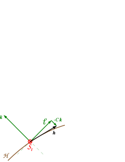
Figure 3: Null vectors $(\bm{\ell},\bm{k})$ associated with the evolution vector $\bm{h}$ by $\bm{h}=\bm{\ell}-C\bm{k}$; the plane of the figure is the plane ${\mathcal{T}}_{p}({\mathcal{S}}_{t})^{\perp}$, so that ${\mathcal{S}}_{t}$ is reduced to a point.

The vectors $\bm{\ell}$ and $\bm{k}$ are necessarily colinear to respectively the vectors $\bm{\tilde{\ell}}$ and $\bm{\tilde{k}}$ associated with the dual-null foliation introduced above, i.e. there exists two positive scalar fields, $A$ and $B$, such that

$$\bm{\ell}=A\bm{\tilde{\ell}}\qquad\mbox{and}\qquad\bm{k}=B\bm{\tilde{k}}.$$ (56)

Actually, we will use Eq. (56) to define $\bm{\ell}$ and $\bm{k}$ away from ${\mathcal{H}}$, Eq. (55) defining them only on ${\mathcal{H}}$. However, all the results presented here are independent of the values of $A$ and $B$ away from ${\mathcal{H}}$. The normalization $\bm{\ell}\cdot\bm{k}=-1$, combined with Eq. (43) relates the product $AB$ to $f$:

$$AB=e^{-f}\qquad\mbox{or}\qquad f=-\ln(AB).$$ (57)

Then, from Eqs. (56) and (46),

$$\bm{\ell}=B^{-1}\bm{\hat{\ell}}\qquad\mbox{and}\qquad\bm{k}=A^{-1}\bm{\hat{k}},$$ (58)

which implies

$$\bm{h}\stackrel{{\scriptstyle{\mathcal{H}}}}{{=}}B^{-1}\bm{\hat{\ell}}-CA^{-1}\bm{\hat{k}}.$$ (59)

Consequently, taking into account Eqs. (42), (46) and (47),

$$\bm{\mathcal{L}}_{\bm{\bm{h}}}\,u\stackrel{{\scriptstyle{\mathcal{H}}}}{{=}}-CA^{-1}\qquad\mbox{and}\qquad\bm{\mathcal{L}}_{\bm{\bm{h}}}\,v\stackrel{{\scriptstyle{\mathcal{H}}}}{{=}}B^{-1}.$$ (60)

On the other side, since $u\stackrel{{\scriptstyle{\mathcal{H}}}}{{=}}u_{0}(t)$ and $v\stackrel{{\scriptstyle{\mathcal{H}}}}{{=}}v_{0}(t)$, $\bm{\mathcal{L}}_{\bm{\bm{h}}}\,u\stackrel{{\scriptstyle{\mathcal{H}}}}{{=}}{u^{\prime}}_{0}(t)$ and $\bm{\mathcal{L}}_{\bm{\bm{h}}}\,v\stackrel{{\scriptstyle{\mathcal{H}}}}{{=}}{v^{\prime}}_{0}(t)$, where we have used the fundamental property $\bm{\mathcal{L}}_{\bm{\bm{h}}}\,t=1$ defining $\bm{h}$ [Eq. (3)]. We then conclude that

$$B\stackrel{{\scriptstyle{\mathcal{H}}}}{{=}}1/{v^{\prime}}_{0}(t)\qquad\mbox{and}\qquad C/A\stackrel{{\scriptstyle{\mathcal{H}}}}{{=}}-{u^{\prime}}_{0}(t).$$ (61)

This implies that, on ${\mathcal{H}}$, the fields $B$ and $C/A$ are functions of $t$ only; in particular, they are constant on each 2-surface ${\mathcal{S}}_{t}$:

$$\bm{\mathcal{D}}B\stackrel{{\scriptstyle{\mathcal{H}}}}{{=}}0\qquad\mbox{and}\qquad\bm{\mathcal{D}}(C/A)\stackrel{{\scriptstyle{\mathcal{H}}}}{{=}}0.$$ (62)

Using Eqs. (56) and (44), we get

$$\bm{\mathrm{d}}\underline{\bm{\ell}}=\bm{\mathrm{d}}\ln A\wedge\underline{\bm{\bm{\ell}}}\qquad\mbox{and}\qquad\bm{\mathrm{d}}\underline{\bm{k}}=\bm{\mathrm{d}}\ln B\wedge\underline{\bm{k}},$$ (63)

from which we obtain

$$\bm{\nabla}_{\bm{\ell}}\,\bm{\ell}=\nu_{(\bm{\ell})}\,\bm{\ell}\qquad\mbox{with}\qquad\nu_{(\bm{\ell})}:=\bm{\mathcal{L}}_{\bm{\bm{\ell}}}\,\ln A,$$ (64)

$$\bm{\nabla}_{\bm{k}}\,\bm{k}=\nu_{(\bm{k})}\,\bm{k}\qquad\mbox{with}\qquad\nu_{(\bm{k})}:=\bm{\mathcal{L}}_{\bm{\bm{k}}}\,\ln B.$$ (65)

$\nu_{(\bm{\ell})}$ and $\nu_{(\bm{k})}$ are the inaffinity parameters of the null vector fields $\bm{\ell}$ and $\bm{k}$. Using the definitions (11), (31) and (32), we then get an expression for the spacetime gradients of $\bm{\ell}$ and $\bm{k}$:

$$\bm{\nabla}\underline{\bm{\ell}}=\bm{\Theta}^{(\bm{\ell})}+\underline{\bm{\ell}}\otimes\bm{\Omega}^{(\bm{\ell})}-\nu_{(\bm{\ell})}\underline{\bm{\ell}}\otimes\underline{\bm{k}}-\bm{\nabla}_{\bm{k}}\underline{\bm{\ell}}\otimes\underline{\bm{\ell}}$$ (66)

$$\bm{\nabla}\underline{\bm{k}}=\bm{\Theta}^{(\bm{k})}-\underline{\bm{k}}\otimes\bm{\Omega}^{(\bm{\ell})}-\nu_{(\bm{k})}\underline{\bm{k}}\otimes\underline{\bm{\ell}}-\bm{\nabla}_{\bm{\ell}}\underline{\bm{k}}\otimes\underline{\bm{k}},$$ (67)

where we have used Eq. (34) with $\sigma=0$ to set $\bm{\Omega}^{(\bm{k})}=-\bm{\Omega}^{(\bm{\ell})}$. Besides, from Eqs. (63) and (62), we get useful identities:

$$\vec{\bm{q}}^{*}\bm{\nabla}_{\bm{k}}\,\underline{\bm{\ell}} = -\bm{\Omega}^{(\bm{\ell})}+\bm{\mathcal{D}}\ln A$$ (68)

$$\vec{\bm{q}}^{*}\bm{\nabla}_{\bm{\ell}}\,\underline{\bm{k}} = \bm{\Omega}^{(\bm{\ell})}.$$ (69)

IV.3 “Surface-gravity” 1-forms

Let us define the 1-form

$$\bm{\kappa}^{(\bm{\ell})}:=\frac{1}{\bm{k}\cdot\bm{\ell}}\,\bm{k}\cdot\bm{\nabla}_{\bm{\stackrel{{\scriptstyle\perp}}{{\vec{q}}}}}\,\bm{\ell}\quad\left[\mbox{or}\ \kappa^{(\bm{\ell})}_{\alpha}:=\frac{1}{k_{\rho}\ell^{\rho}}k_{\mu}\nabla_{\nu}\ell^{\mu}\,{\stackrel{{\scriptstyle\perp}}{{q}}}^{\nu}_{\ \,\alpha}\right],$$ (70)

where $\bm{\stackrel{{\scriptstyle\perp}}{{\vec{q}}}}$ denotes the orthogonal projector on the vector plane ${\mathcal{T}}_{p}({\mathcal{S}}_{t})^{\perp}$, i.e. the complementary of $\bm{\vec{q}}$: $\bm{1}=\bm{\vec{q}}\,+\bm{\stackrel{{\scriptstyle\perp}}{{\vec{q}}}}$. The definition (70) is similar to the definition (31) of $\bm{\Omega}^{(\bm{\ell})}$, except for $\bm{\vec{q}}$ replaced by $\bm{\stackrel{{\scriptstyle\perp}}{{\vec{q}}}}$. Hence, whereas $\bm{\Omega}^{(\bm{\ell})}$ was defined for a single 2-surface ${\mathcal{S}}_{t}$, $\bm{\kappa}^{(\bm{\ell})}$ requires the knowledge of the null normal $\bm{\ell}$ in directions normal to ${\mathcal{S}}_{t}$. From Eq. (64) and (65), the inaffinity parameters $\nu_{(\bm{\ell})}$ and $\nu_{(\bm{k})}$ are recovered by applying the 1-form $\bm{\kappa}^{(\bm{\ell})}$ to respectively $\bm{\ell}$ and $-\bm{k}$:

$$\langle\bm{\kappa}^{(\bm{\ell})},\bm{\ell}\rangle=\nu_{(\bm{\ell})}\qquad\mbox{and}\qquad\langle\bm{\kappa}^{(\bm{\ell})},\bm{k}\rangle=-\nu_{(\bm{k})}.$$ (71)

A useful relation is then

$$\langle\bm{\kappa}^{(\bm{\ell})},\bm{h}\rangle=\nu_{(\bm{\ell})}+C\nu_{(\bm{k})}.$$ (72)

IV.4 Trapping horizons and dynamical horizons

Let us recall here the various definitions involved in the local characterizations of black holes mentioned in the Introduction. The hypersurface ${\mathcal{H}}$ equipped with the spacelike foliation $({\mathcal{S}}_{t})_{t\in\mathbb{R}}$ is called a marginally outer trapped tube (MOTT) Booth05 if each leaf ${\mathcal{S}}_{t}$ is a marginal outer trapped surface (cf. Sec. III.2), i.e. if $\theta^{\bm{\ell}}=0$ at any point in ${\mathcal{H}}$. Following Hayward Haywa94b a trapping horizon is a MOTT on which $\theta^{(\bm{k})}\not=0$ and $\bm{\mathcal{L}}_{\bm{k}}\,\theta^{(\bm{\ell})}\not=0$, being qualified as future trapped horizon if $\theta^{(\bm{k})}<0$ and future outer trapped horizon (FOTH) if $\theta^{(\bm{k})}<0$ and $\bm{\mathcal{L}}_{\bm{k}}\,\theta^{(\bm{\ell})}<0$, the latter subcase being the one relevant for black holes (see Ref. Booth05 for a discussion). The dynamical horizons introduced by Ashtekar and Krishnan AshteK02 ; AshteK03 ; AshteK04 are MOTT such that (i) ${\mathcal{H}}$ is spacelike and (ii) $\theta^{(\bm{k})}<0$. In particular, a spacelike future trapping horizon is a dynamical horizon. When it is null, a MOTT is called a non-expanding horizon Hajic73 ; Hajic75 ; AshteBL02 . It corresponds to a black hole in equilibrium.

V The generalized Damour-Navier-Stokes equation

V.1 Original Damour-Navier-Stokes equation

In the case where the hypersurface ${\mathcal{H}}$ is null, and in particular when ${\mathcal{H}}$ is the event horizon of a black hole, $\bm{h}=\bm{\ell}$ and the Damour-Navier-Stokes equation Damou79 ; Damou82 ; ParikW98 ; GourgJ05 writes

$${}^{{\mathcal{S}}}\!\bm{\mathcal{L}}_{\bm{\bm{\ell}}}\,\bm{\Omega}^{(\bm{\ell})}+\theta^{(\bm{\ell})}\bm{\Omega}^{(\bm{\ell})} = \bm{\mathcal{D}}\nu_{(\bm{\ell})}-\bm{\mathcal{D}}\cdot\vec{\bm{\sigma}}^{(\bm{\ell})}+\frac{1}{2}\bm{\mathcal{D}}\theta^{(\bm{\ell})}$$ (73)

$$+8\pi\vec{\bm{q}}^{*}\bm{T}\cdot\bm{\ell}.$$

This equation is derived from the Einstein equation, as the presence of the stress-energy tensor $\bm{T}$ testifies. It has exactly the same structure as a 2-dimensional Navier-Stokes equation: dividing Eq. (73) by $8\pi$, $-\bm{\Omega}^{(\bm{\ell})}/(8\pi)$ is interpreted by Damour Damou79 ; Damou82 as a momentum surface density, $\nu_{(\bm{\ell})}/(8\pi)$ as a “fluid” pressure, $1/(16\pi)$ as a shear viscosity ($\bm{\sigma}^{(\bm{\ell})}$ being the shear tensor), $-1/(16\pi)$ in front of $\bm{\mathcal{D}}\theta^{(\bm{\ell})}$ as a bulk viscosity and $\vec{\bm{q}}^{*}\bm{T}\cdot\bm{\ell}$ as a force surface density. The reader is referred to Chap. VI of Ref. ThornPM86 for an extended discussion of this “viscous fluid” viewpoint.

V.2 Derivation of the generalized equation

First of all, it must be noted that in the Damour-Navier-Stokes equation (73), the vector field $\bm{\ell}$ plays two different roles: it is both the evolution vector along ${\mathcal{H}}$ (obviously in a term like ${}^{{\mathcal{S}}}\!\bm{\mathcal{L}}_{\bm{\bm{\ell}}}\,$) and the normal to ${\mathcal{H}}$ (in a term like $\vec{\bm{q}}^{*}\bm{T}\cdot\bm{\ell}$). When ${\mathcal{H}}$ is no longer null, these two roles have to be taken by two different vectors. We have already seen that the privileged evolution vector along ${\mathcal{H}}$ is the vector $\bm{h}$ associated with the foliation $({\mathcal{S}}_{t})_{t\in\mathbb{R}}$. Regarding the normal vector, it is natural to consider

$$\bm{m}:=\bm{\ell}+C\bm{k}.$$ (74)

Indeed this vector is normal to ${\mathcal{H}}$, since by construction $\bm{m}\in{\mathcal{T}}_{p}({\mathcal{S}}_{t})^{\perp}$ and $\bm{m}\cdot\bm{h}=0$, and in the limit where ${\mathcal{H}}$ is null, it reduces to $\bm{\ell}$. It can be viewed as the unique normal vector to ${\mathcal{H}}$ whose projection onto ${\mathcal{H}}$ along the ingoing null direction $\bm{k}$ is $\bm{h}$ (see Fig. 4). Note that the scalar square of $\bm{m}$ is the negative of that of $\bm{h}$:

$$\bm{m}\cdot\bm{m}=-2C=-\bm{h}\cdot\bm{h}.$$ (75)

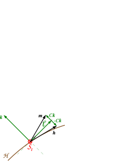
Figure 4: Same as Fig. 3 but with in addition the vector $\bm{m}$ normal to the hypersurface ${\mathcal{H}}$.

A generalization of the Damour-Navier-Stokes equation to the non-null case should contain the term $\vec{\bm{q}}^{*}\bm{T}\cdot\bm{m}$, instead of $\vec{\bm{q}}^{*}\bm{T}\cdot\bm{\ell}$, in the right-hand side. By virtue of Einstein equation and the fact that $\vec{\bm{q}}(\bm{m})=0$, $8\pi\vec{\bm{q}}^{*}\bm{T}\cdot\bm{m}=\vec{\bm{q}}^{*}\bm{R}\cdot\bm{m}$, where $\bm{R}$ is the Ricci tensor associated with the spacetime metric $\bm{g}$. The starting point for getting the generalized Damour-Navier-Stokes equation will be then the contracted Ricci identity applied to the vector $\bm{m}$ and projected onto ${\mathcal{S}}_{t}$:

$$\left(\nabla_{\mu}\nabla_{\nu}m^{\mu}-\nabla_{\nu}\nabla_{\mu}m^{\mu}\right)q^{\nu}_{\ \,\alpha}=R_{\mu\nu}m^{\mu}q^{\nu}_{\ \,\alpha}.$$ (76)

Now, by combining definition (74) with expressions (66) and (67),

$$\nabla_{\alpha}m^{\beta} = \Theta_{\alpha}^{(\bm{m})\beta}+\Omega_{\alpha}^{(\bm{\ell})}h^{\beta}-\nu_{(\bm{\ell})}k_{\alpha}\ell^{\beta}-C\nu_{(\bm{k})}\ell_{\alpha}k^{\beta}$$ (77)

$$-\ell_{\alpha}k^{\sigma}\nabla_{\sigma}\ell^{\beta}-Ck_{\alpha}\ell^{\sigma}\nabla_{\sigma}k^{\beta}+\nabla_{\alpha}Ck^{\beta}.$$

Substituting Eq. (77) for $\nabla_{\nu}m^{\mu}$ and $\nabla_{\mu}m^{\mu}$ in Eq. (76), expanding and making use of identities (68), (69) and (72) yields, after some rearrangements,

$$R_{\mu\nu}m^{\mu}q^{\nu}_{\ \,\alpha} = q^{\nu}_{\ \,\alpha}\nabla_{\mu}\Theta_{\nu}^{(\bm{m})\mu}+q^{\nu}_{\ \,\alpha}h^{\mu}\nabla_{\mu}\Omega_{\nu}^{(\bm{\ell})}+\Theta_{\alpha}^{(\bm{h})\mu}\,\Omega_{\mu}^{(\bm{\ell})}+\theta^{(\bm{h})}\,\Omega_{\alpha}^{(\bm{\ell})}-\mathcal{D}_{\alpha}\left(\theta^{(\bm{m})}+\langle\bm{\kappa}^{(\bm{\ell})},\bm{h}\rangle\right)-\Theta_{\alpha}^{(\bm{\ell})\mu}\,\mathcal{D}_{\mu}\ln A$$ (78)

$$-\Theta_{\alpha}^{(\bm{k})\mu}\,\mathcal{D}_{\mu}C+\theta^{(\bm{k})}\mathcal{D}_{\alpha}C+\nu_{(\bm{k})}\underbrace{\left(\mathcal{D}_{\alpha}C-C\mathcal{D}_{\alpha}\ln A\right)}_{=0},$$

where the “$=0$” results from Eq. (62). Now, from the relation (25) between the derivatives $\bm{\bm{\mathcal{D}}}$ and $\bm{\nabla}$, one has [making use of identities (68) and (69)]

$$q^{\nu}_{\ \,\alpha}\nabla_{\mu}\Theta_{\nu}^{(\bm{m})\mu}=\mathcal{D}_{\mu}\Theta_{\alpha}^{(\bm{m})\mu}+\Theta_{\alpha}^{(\bm{m})\mu}\,\mathcal{D}_{\mu}\ln A.$$ (79)

Besides, expressing the Lie derivative in terms of $\bm{\nabla}$ gives

$$q^{\nu}_{\ \,\alpha}{\mathcal{L}}_{\bm{\bm{h}}}\,\Omega_{\nu}^{(\bm{\ell})}=q^{\nu}_{\ \,\alpha}h^{\mu}\nabla_{\mu}\Omega_{\nu}^{(\bm{\ell})}+\Theta_{\alpha}^{(\bm{h})\mu}\,\Omega_{\mu}^{(\bm{\ell})}.$$ (80)

Thanks to Eqs. (79) and (80), Eq. (78) reduces to

$$R_{\mu\nu}m^{\mu}q^{\nu}_{\ \,\alpha}=\mathcal{D}_{\mu}\Theta_{\alpha}^{(\bm{m})\mu}+q^{\nu}_{\ \,\alpha}{\mathcal{L}}_{\bm{\bm{h}}}\,\Omega_{\nu}^{(\bm{\ell})}+\theta^{(\bm{h})}\,\Omega_{\alpha}^{(\bm{\ell})}-\mathcal{D}_{\alpha}\left(\theta^{(\bm{m})}+\langle\bm{\kappa}^{(\bm{\ell})},\bm{h}\rangle\right)+\theta^{(\bm{k})}\mathcal{D}_{\alpha}C,$$ (81)

where Eq. (62) has been used to set to zero the term $\Theta_{\alpha}^{(\bm{k})\mu}\left(C\mathcal{D}_{\mu}\ln A-\mathcal{D}_{\mu}C\right)$ which had appeared. Now, from Eq. (8) and the property $\vec{\bm{q}}^{*}\bm{\Omega}^{(\bm{\ell})}=\bm{\Omega}^{(\bm{\ell})}$, the term $\vec{\bm{q}}^{*}\bm{\mathcal{L}}_{\bm{\bm{h}}}\,\bm{\Omega}^{(\bm{\ell})}$ which appears in the above equation is nothing but ${}^{{\mathcal{S}}}\!\bm{\mathcal{L}}_{\bm{\bm{h}}}\,\bm{\Omega}^{(\bm{\ell})}$. Re-expressing $\bm{\Theta}^{(\bm{m})}$ in terms of the shear tensor $\bm{\sigma}^{(\bm{m})}$ and the expansion scalar $\theta^{(\bm{m})}$ via Eq. (14) and taking account the Einstein equation then leads to

$${}^{{\mathcal{S}}}\!\bm{\mathcal{L}}_{\bm{\bm{h}}}\,\bm{\Omega}^{(\bm{\ell})}+\theta^{(\bm{h})}\,\bm{\Omega}^{(\bm{\ell})}=\bm{\mathcal{D}}\langle\bm{\kappa}^{(\bm{\ell})},\bm{h}\rangle-\bm{\mathcal{D}}\cdot\vec{\bm{\sigma}}^{(\bm{m})}+\frac{1}{2}\bm{\mathcal{D}}\theta^{(\bm{m})}-\theta^{(\bm{k})}\bm{\mathcal{D}}C+8\pi\vec{\bm{q}}^{*}\bm{T}\cdot\bm{m}.$$ (82)

This is the generalization of Damour-Navier-Stokes equation to the case where the foliated hypersurface ${\mathcal{H}}$ is not necessarily null. In the null limit, $C=0$, $\bm{h}=\bm{m}=\bm{\ell}$ and we recover Damour’s original version, i.e. Eq. (73). In the non-null case, it is worth to notice that the obtained equation is not much more complicated than Eq. (73): apart from substitutions of $\bm{\ell}$ by either $\bm{h}$ or $\bm{m}$, as discussed above, it contains only one extra term: $\theta^{(\bm{k})}\bm{\mathcal{D}}C$.

V.3 Change of normal fundamental form

Let us rewrite the generalized Damour-Navier-Stokes equation in terms of the normal fundamental form $\bm{\Omega}^{(\bm{\ell}^{\prime})}$ associated with a generic null vector $\bm{\ell}^{\prime}$, instead of $\bm{\ell}$. Setting $\bm{\bm{\ell}}^{\prime}=\lambda\bm{\ell}$, with $\lambda>0$, $\bm{\Omega}^{(\bm{\ell}^{\prime})}$ is related to $\bm{\Omega}^{(\bm{\ell})}$ by Eq. (40), from which we deduce

$${}^{{\mathcal{S}}}\!\bm{\mathcal{L}}_{\bm{\bm{h}}}\,\bm{\Omega}^{(\bm{\ell}^{\prime})} + \theta^{(\bm{h})}\,\bm{\Omega}^{(\bm{\ell}^{\prime})}={}^{{\mathcal{S}}}\!\bm{\mathcal{L}}_{\bm{\bm{h}}}\,\bm{\Omega}^{(\bm{\ell})}+\theta^{(\bm{h})}\,\bm{\Omega}^{(\bm{\ell})}$$ (83)

$$+\bm{\mathcal{D}}\left(\bm{\mathcal{L}}_{\bm{\bm{h}}}\,\ln\lambda\right)+\theta^{(\bm{h})}\bm{\mathcal{D}}\ln\lambda,$$

where we have used ${}^{{\mathcal{S}}}\!\bm{\mathcal{L}}_{\bm{\bm{h}}}\,\bm{\mathcal{D}}\ln\lambda=\bm{\mathcal{D}}(\bm{\mathcal{L}}_{\bm{\bm{h}}}\,\ln\lambda)$. Besides, we note that the 1-form $\bm{\kappa}^{(\bm{\ell})}$ transforms as follows

$$\bm{\kappa}^{(\bm{\ell}^{\prime})}=\bm{\kappa}^{(\bm{\ell})}+\bm{\nabla}_{\bm{\stackrel{{\scriptstyle\perp}}{{\vec{q}}}}}\ln\lambda,$$ (84)

from which

$$\bm{\mathcal{D}}\langle\bm{\kappa}^{(\bm{\ell}^{\prime})},\bm{h}\rangle=\bm{\mathcal{D}}\langle\bm{\kappa}^{(\bm{\ell})},\bm{h}\rangle+\bm{\mathcal{D}}\left(\bm{\mathcal{L}}_{\bm{\bm{h}}}\,\ln\lambda\right).$$ (85)

Combining Eqs. (82), (83) and (85), and using $\theta^{(\bm{h})}=\theta^{(\bm{\ell})}-C\theta^{(\bm{k})}$ yields

$${}^{{\mathcal{S}}}\!\bm{\mathcal{L}}_{\bm{\bm{h}}}\,\bm{\Omega}^{(\bm{\ell}^{\prime})}+\theta^{(\bm{h})}\,\bm{\Omega}^{(\bm{\ell}^{\prime})}=\bm{\mathcal{D}}\langle\bm{\kappa}^{(\bm{\ell}^{\prime})},\bm{h}\rangle-\bm{\mathcal{D}}\cdot\vec{\bm{\sigma}}^{(\bm{m})}+\frac{1}{2}\bm{\mathcal{D}}\theta^{(\bm{m})}+\theta^{(\bm{\ell})}\bm{\mathcal{D}}\ln\lambda-\theta^{(\bm{k})}\left(\bm{\mathcal{D}}C+C\bm{\mathcal{D}}\ln\lambda\right)+8\pi\vec{\bm{q}}^{*}\bm{T}\cdot\bm{m}.$$ (86)

If we chose $\lambda=A^{-1}$, then by virtue of Eq. (62), the term $\bm{\mathcal{D}}C+C\bm{\mathcal{D}}\ln\lambda$ vanishes identically. Since $\lambda=A^{-1}$ corresponds to $\bm{\ell}^{\prime}=\bm{\tilde{\ell}}$ [cf. Eq. (56)], Eq. (86) reduces then to

$${}^{{\mathcal{S}}}\!\bm{\mathcal{L}}_{\bm{\bm{h}}}\,\bm{\Omega}^{(\bm{\tilde{\ell}})}+\theta^{(\bm{h})}\,\bm{\Omega}^{(\bm{\tilde{\ell}})}=\bm{\mathcal{D}}\langle\bm{\kappa}^{(\bm{\tilde{\ell}})},\bm{h}\rangle-\bm{\mathcal{D}}\cdot\vec{\bm{\sigma}}^{(\bm{m})}+\frac{1}{2}\bm{\mathcal{D}}\theta^{(\bm{m})}-\theta^{(\bm{\ell})}\bm{\mathcal{D}}\ln A+8\pi\vec{\bm{q}}^{*}\bm{T}\cdot\bm{m}.$$ (87)

In the case where ${\mathcal{H}}$ is not null ($C\not=0$), another way to set to zero the term $\bm{\mathcal{D}}C+C\bm{\mathcal{D}}\ln\lambda$ in Eq. (86) is to choose

$$\lambda=F(t)/|C|,$$ (88)

where $F(t)$ is an arbitrary function of $t$, since then $\bm{\mathcal{D}}C+C\bm{\mathcal{D}}\ln\lambda=C\bm{\mathcal{D}}\ln(\lambda|C|)=C\bm{\mathcal{D}}\ln F(t)=0$. The simplest choice $F(t)=1$ corresponds to the following decomposition of the evolution vector: $\bm{h}=\pm(C\bm{\ell}^{\prime}-\bm{k}^{\prime})$ (with $\pm$ corresponding to $C>0$ and $C<0$ respectively), to be contrasted with the decomposition (55). Actually this amounts simply to swapping the vectors $\bm{\ell}$ and $\bm{k}$.

V.4 Application to trapping horizons

If ${\mathcal{H}}$ is a trapping horizon (or more generally a MOTT, cf. Sec. IV.4), then $\theta^{(\bm{\ell})}=0$ and Eq. (87) becomes

$${}^{{\mathcal{S}}}\!\bm{\mathcal{L}}_{\bm{\bm{h}}}\,\bm{\Omega}^{(\bm{\tilde{\ell}})}+\theta^{(\bm{h})}\,\bm{\Omega}^{(\bm{\tilde{\ell}})}=\bm{\mathcal{D}}\langle\bm{\kappa}^{(\bm{\tilde{\ell}})},\bm{h}\rangle-\bm{\mathcal{D}}\cdot\vec{\bm{\sigma}}^{(\bm{m})}$$

$$\ \quad+\frac{1}{2}\bm{\mathcal{D}}\theta^{(\bm{m})}+8\pi\vec{\bm{q}}^{*}\bm{T}\cdot\bm{m}.$$ (89)

This equation is structurally identical to the original Damour-Navier-Stokes equation [Eq. (73)]: apart from substitutions of $\bm{\ell}$ by either $\bm{h}$ or $\bm{m}$, it does not contain any extra term. The differences are that the original Damour-Navier-Stokes applies to a null ${\mathcal{H}}$ but with $\theta^{(\bm{\ell})}$ not necessarily zero, whereas Eq. (89) is valid for both ${\mathcal{H}}$ null or spacelike, but assumes $\theta^{(\bm{\ell})}=0$.

VI Angular momentum

Traditionally the concept of angular momentum is a global one and requires the evaluation of a Komar integral at spatial infinity, assuming ${\mathcal{M}}$ to be asymptotically flat and endowed with an axisymmetric Killing vector (cf. e.g. Ref. Poiss04 ). However, by means of some Hamiltonian analysis, the concept of angular momentum can be made quasilocal, as a quantity associated with the interior of the spacetime region delimited by the hypersurface ${\mathcal{H}}$. The prototype of such quasilocal formulation is Brown-York analysis BrownY93 which will be taken as the starting point for our discussion.

VI.1 Brown-York angular momentum

Let us assume that the hypersurface ${\mathcal{H}}$ is timelike and is axisymmetric, with the associated Killing vector $\bm{\varphi}$ lying in the 2-surfaces ${\mathcal{S}}_{t}$. The definition of angular momentum by Brown and York BrownY93 is then

$$J:=\oint_{{\mathcal{S}}_{t}}\langle\bm{j},\bm{\varphi}\rangle\,{}^{\scriptscriptstyle\mathcal{S}}\!\bm{\epsilon},$$ (90)

where ${}^{\scriptscriptstyle\mathcal{S}}\!\bm{\epsilon}$ is the surface element of ${\mathcal{S}}_{t}$ associated with the induced metric $\bm{q}$ (${}^{\scriptscriptstyle\mathcal{S}}\!\bm{\epsilon}=\sqrt{q}\,\bm{\mathrm{d}}x^{2}\wedge\bm{\mathrm{d}}x^{3}$ for any coordinate system $x^{a}=(x^{2},x^{3})$ on ${\mathcal{S}}_{t}$, with $q:=\det q_{ab}$) and the momentum surface density 1-form $\bm{j}$ is defined as follows. Adopting a 3+1 perspective (cf. Sec. 1), let $\Sigma_{t}$ be a spacelike hypersurface intersecting ${\mathcal{H}}$ in ${\mathcal{S}}_{t}$. Denoting by $\bm{\gamma}$ and $\bm{K}$ the induced metric and extrinsic curvature tensor of $\Sigma_{t}$, $\bm{j}$ is expressible as

$$j_{\alpha}=-\frac{2}{\sqrt{\gamma}}P^{\mu\nu}s_{\mu}q_{\nu\alpha},$$ (91)

where $\bm{s}$ is the unit spacelike normal to ${\mathcal{S}}_{t}$ which lies in $\Sigma_{t}$ and $\bm{P}$ is the momentum canonically conjugate to $\bm{\gamma}$:

$$P^{\alpha\beta}=\frac{1}{16\pi}\sqrt{\gamma}\left(K\gamma^{\alpha\beta}-K^{\alpha\beta}\right).$$ (92)

Since $\bm{K}$ is related to the gradient of the timelike unit normal to $\Sigma_{t}$, $\bm{n}$, by $K_{\alpha\beta}=-\nabla_{\mu}n_{\nu}\,\gamma^{\mu}_{\ \,\alpha}\gamma^{\nu}_{\ \,\beta}$, we get, by inserting Eq. (92) in Eq. (91) and comparing with Eq. (29),

$$\bm{j}=-\frac{1}{8\pi}\bm{\Omega}^{(\bm{n})}.$$ (93)

By considering the null vector $\bm{\ell}^{\prime}:=\bm{n}+\bm{s}$ and combining the transformation laws (35) and (40), one gets

$$\bm{j}=-\frac{1}{8\pi}\left(\bm{\Omega}^{(\bm{\ell})}+\bm{\mathcal{D}}\ln\lambda\right),$$ (94)

where $\lambda$ is the scale factor relating $\bm{\ell}$ to $\bm{n}+\bm{s}$: $\bm{n}+\bm{s}=\lambda\bm{\ell}$. Now, the Killing equation for the vector $\bm{\varphi}$ and the fact that $\bm{\varphi}\in{\mathcal{T}}({\mathcal{S}}_{t})$ imply $\bm{\mathcal{D}}\cdot\bm{\varphi}=0$. Consequently $\bm{\varphi}\cdot\bm{\mathcal{D}}\ln\lambda=\bm{\mathcal{D}}\cdot(\ln\lambda\,\bm{\varphi})$ is a perfect divergence, the integral of which over the closed surface ${\mathcal{S}}_{t}$ vanishes. Therefore substituting Eq. (94) for $\bm{j}$ into Eq. (90) yields

$$J=-\frac{1}{8\pi}\oint_{{\mathcal{S}}_{t}}\langle\bm{\Omega}^{(\bm{\ell})},\bm{\varphi}\rangle\,{}^{\scriptscriptstyle\mathcal{S}}\!\bm{\epsilon}.$$ (95)

This expression is in perfect agreement with the interpretation of $-\bm{\Omega}^{(\bm{\ell})}/(8\pi)$ as a momentum surface density performed in Sec. V.

VI.2 Generalized angular momentum

It may be noticed that the timelike character of the hypersurface ${\mathcal{H}}$, assumed in Brown-York Hamiltonian analysis BrownY93 , does not play any role in the expression (95) of the angular momentum. Actually the definition of angular momentum, based on Eq. (95), has been extended to null hypersurfaces by Booth Booth01 (in a generalization of Brown-York analysis) and Ashtekar et al. AshteBL01 (in the framework of isolated horizons).

It is also worth to notice that the independence of the integral defining $J$ with respect to the normal fundamental form (i.e. $\bm{\Omega}^{(\bm{n})}$ or $\bm{\Omega}^{(\bm{\ell})}$) stems only from the divergence-free property of the vector $\bm{\varphi}$, which is a condition weaker than that of being a Killing vector. Therefore, one may relax the later and follow Booth and Fairhurst’s recent analysis BoothF05 to introduce a generalized angular momentum as follows. Let us assume that the 2-surfaces ${\mathcal{S}}_{t}$ have the topology of $\mathbb{S}^{2}$. Let $\bm{\varphi}$ be a vector field in ${\mathcal{T}}({\mathcal{S}}_{t})$ which (i) has closed orbits and (ii) has vanishing divergence with respect to the induced connection $\bm{\mathcal{D}}$:

$$\bm{\mathcal{D}}\cdot\bm{\varphi}=0.$$ (96)

The angular momentum associated with $\bm{\varphi}$ is then defined by BoothF05

$$J(\bm{\varphi}):=-\frac{1}{8\pi}\oint_{{\mathcal{S}}_{t}}\langle\bm{\Omega}^{(\bm{\ell})},\bm{\varphi}\rangle\,{}^{\scriptscriptstyle\mathcal{S}}\!\bm{\epsilon},$$ (97)

which is a formula structurally identical to formula (95). The main difference is that $\bm{\varphi}$ is no longer the Killing vector reflecting the axisymmetry of ${\mathcal{S}}_{t}$ and uniquely defined by the normalization of the orbit lengths to $2\pi$, but merely a divergence-free vector field. Consequently, $J$ depends on the choice of $\bm{\varphi}$. However formula (97) shares with formula (95) the independence with respect to the choice of the normal fundamental form $\bm{\Omega}^{(\bm{\ell})}$, thanks to the divergence-free character of $\bm{\varphi}$. Indeed, under a change of null normal $\bm{\ell}^{\prime}=\lambda\bm{\ell}$, $\bm{\Omega}^{(\bm{\ell})}$ is changed to $\bm{\Omega}^{(\bm{\ell}^{\prime})}=\bm{\Omega}^{(\bm{\ell})}+\bm{\mathcal{D}}\ln\lambda$ [Eq. (40)] and since $\bm{\mathcal{D}}\cdot\bm{\varphi}=0$, $\bm{\varphi}\cdot\bm{\mathcal{D}}\ln\lambda=\bm{\mathcal{D}}\cdot(\ln\lambda\,\bm{\varphi})$ is a perfect divergence, the integral of which on ${\mathcal{S}}_{t}$ vanishes.

As a further justification of definition (97), it is shown in Appendix A that, when ${\mathcal{H}}$ is a dynamical horizon, $J(\bm{\varphi})$ agrees with the generalized angular momentum defined by Ashtekar and Krishnan AshteK03 ; AshteK04 .

VI.3 Angular momentum flux law

For any 1-form $\bm{\omega}$ and vector field $\bm{\varphi}$ defined on ${\mathcal{H}}$ and both tangent to ${\mathcal{S}}_{t}$ for all $t\in\mathbb{R}$, the following identity holds:

$$\frac{d}{dt}\oint_{{\mathcal{S}}_{t}}\langle\bm{\omega},\bm{\varphi}\rangle\,{}^{\scriptscriptstyle\mathcal{S}}\!\bm{\epsilon} = \oint_{{\mathcal{S}}_{t}}{}^{{\mathcal{S}}}\!\bm{\mathcal{L}}_{\bm{h}}\,\!\left[\langle\bm{\omega},\bm{\varphi}\rangle\,{}^{\scriptscriptstyle\mathcal{S}}\!\bm{\epsilon}\right]$$ (98)

$$= \oint_{{\mathcal{S}}_{t}}\langle{}^{{\mathcal{S}}}\!\bm{\mathcal{L}}_{\bm{h}}\,\bm{\omega}+\theta^{(\bm{h})}\bm{\omega},\bm{\varphi}\rangle{}^{\scriptscriptstyle\mathcal{S}}\!\bm{\epsilon}$$

$$+\oint_{{\mathcal{S}}_{t}}\langle\bm{\omega},\bm{\mathcal{L}}_{\bm{h}}\,\bm{\varphi}\rangle{}^{\scriptscriptstyle\mathcal{S}}\!\bm{\epsilon},$$

where the first equality results from the Lie transport of the 2-surfaces ${\mathcal{S}}_{t}$ by the vector field $\bm{h}$ (cf. Sec. II.2) and in the second equality the relation $\bm{\mathcal{L}}_{\bm{h}}\,{}^{\scriptscriptstyle\mathcal{S}}\!\bm{\epsilon}=\theta^{(\bm{h})}{}^{\scriptscriptstyle\mathcal{S}}\!\bm{\epsilon}$ has been used [cf. Eq. (15)].

Applying the above identity to the 1-form $\bm{\omega}=\bm{\Omega}^{(\bm{\ell})}$ and employing the generalized Damour-Navier-Stokes equation (82) leads to an evolution equation for the generalized angular momentum $J(\bm{\varphi})$ defined by Eq. (97):

$$\frac{d}{dt}J(\bm{\varphi})=-\oint_{{\mathcal{S}}_{t}}\bm{T}(\bm{m},\bm{\varphi})\,{}^{\scriptscriptstyle\mathcal{S}}\!\bm{\epsilon}-\frac{1}{16\pi}\oint_{{\mathcal{S}}_{t}}\left[\stackrel{{\scriptstyle\twoheadrightarrow}}{{\bm{\sigma}}}\!\!{}^{(\bm{m})}\!:\bm{\mathcal{L}}_{\bm{\varphi}}\,\bm{q}-2\theta^{(\bm{k})}\bm{\varphi}\cdot\bm{\mathcal{D}}C\right]{}^{\scriptscriptstyle\mathcal{S}}\!\bm{\epsilon}-\frac{1}{8\pi}\oint_{{\mathcal{S}}_{t}}\langle\bm{\Omega}^{(\bm{\ell})},\bm{\mathcal{L}}_{\bm{h}}\,\bm{\varphi}\rangle{}^{\scriptscriptstyle\mathcal{S}}\!\bm{\epsilon}.$$ (99)

The notation ‘$:$’ stands for a complete contraction, whereas the double arrow means that the two indices of $\bm{\sigma}^{(\bm{m})}$ have been raised with the metric $\bm{g}$: $\stackrel{{\scriptstyle\twoheadrightarrow}}{{\bm{\sigma}}}\!\!{}^{(\bm{m})}\!:\bm{\mathcal{L}}_{\bm{\varphi}}\,\bm{q}=\sigma^{(\bm{m})ab}{\mathcal{L}}_{\bm{\varphi}}\,q_{ab}$. The integrals involving the pure gradients $\bm{\mathcal{D}}\langle\kappa^{(\bm{\ell})},\bm{h}\rangle$ and $\bm{\mathcal{D}}\theta^{(\bm{m})}$ have been set to zero thanks to the property $\bm{\mathcal{D}}\cdot\bm{\varphi}=0$. Besides, we have written $\bm{\varphi}\cdot\left(\bm{\mathcal{D}}\cdot\vec{\bm{\sigma}}^{(\bm{m})}\right)=\bm{\mathcal{D}}\cdot\left(\vec{\bm{\sigma}}^{(\bm{m})}\cdot\bm{\varphi}\right)-\vec{\bm{\sigma}}^{(\bm{m})}:\bm{\mathcal{D}}\bm{\varphi}$, with the integral of the divergence $\bm{\mathcal{D}}\cdot\left(\vec{\bm{\sigma}}^{(\bm{m})}\cdot\bm{\varphi}\right)$ being zero since ${\mathcal{S}}_{t}$ is a closed manifold and, thanks to the symmetry of the shear tensor $\bm{\sigma}^{(\bm{m})}$, $2\vec{\bm{\sigma}}^{(\bm{m})}:\bm{\mathcal{D}}\bm{\varphi}=\sigma^{(\bm{m})ab}(\mathcal{D}_{a}\varphi_{b}+\mathcal{D}_{b}\varphi_{a})=\stackrel{{\scriptstyle\twoheadrightarrow}}{{\bm{\sigma}}}\!\!{}^{(\bm{m})}\!:\bm{\mathcal{L}}_{\bm{\varphi}}\,\bm{q}$.

The last integral in Eq. (99) occurs to take into account a possible variation of $\bm{\varphi}$ along the evolution vector $\bm{h}$. To make the variation of $J$ more meaningful, it is natural to demand that the vector field $\bm{\varphi}$ is transported by $\bm{h}$:

$$\bm{\mathcal{L}}_{\bm{h}}\,{\bm{\varphi}}=0.$$ (100)

From now on, we assume that $\bm{\varphi}$ obeys to both conditions (96) and (100). Note that if $\bm{\varphi}$ is a symmetry generator of ${\mathcal{H}}$ which is tangent to ${\mathcal{S}}_{t}$, these two conditions are satisfied (in particular $\bm{\mathcal{L}}_{\bm{h}}\,\bm{\varphi}=-\bm{\mathcal{L}}_{\bm{\varphi}}\,\bm{h}=0$). Then Eq. (99) simplifies to

$$\frac{d}{dt}J(\bm{\varphi})=-\oint_{{\mathcal{S}}_{t}}\bm{T}(\bm{m},\bm{\varphi})\,{}^{\scriptscriptstyle\mathcal{S}}\!\bm{\epsilon}-\frac{1}{16\pi}\oint_{{\mathcal{S}}_{t}}\left[\stackrel{{\scriptstyle\twoheadrightarrow}}{{\bm{\sigma}}}\!\!{}^{(\bm{m})}\!:\bm{\mathcal{L}}_{\bm{\varphi}}\,\bm{q}-2\theta^{(\bm{k})}\bm{\varphi}\cdot\bm{\mathcal{D}}C\right]{}^{\scriptscriptstyle\mathcal{S}}\!\bm{\epsilon}.$$ (101)

In the case where ${\mathcal{H}}$ is a null hypersurface, then $C=0$ and Eq. (101) reduces to

$$\frac{d}{dt}J(\bm{\varphi})=-\oint_{{\mathcal{S}}_{t}}\bm{T}(\bm{\ell},\bm{\varphi})\,{}^{\scriptscriptstyle\mathcal{S}}\!\bm{\epsilon}-\frac{1}{16\pi}\oint_{{\mathcal{S}}_{t}}\stackrel{{\scriptstyle\twoheadrightarrow}}{{\bm{\sigma}}}\!\!{}^{(\bm{\ell})}\!:\bm{\mathcal{L}}_{\bm{\varphi}}\,\bm{q}\;{}^{\scriptscriptstyle\mathcal{S}}\!\bm{\epsilon}.$$ (102)

We recover here Eq. (6.134) of the Membrane Paradigm book ThornPM86 , where the first term is interpreted as the variation of $J$ due to the flux of angular momentum carried by matter and electromagnetic field at ${\mathcal{H}}$ and the second term accounts for the shear viscosity of ${\mathcal{H}}$.

Let us consider now the case where ${\mathcal{H}}$ is either timelike or spacelike: $C\not=0$ and we may express $\theta^{(\bm{k})}$ in Eq. (101) as $\theta^{(\bm{k})}=\left(\theta^{(\bm{\ell})}-\theta^{(\bm{h})}\right)/C$ [cf. Eq. (55)], so that

$$-\theta^{(\bm{k})}\bm{\varphi}\cdot\bm{\mathcal{D}}C=-\theta^{(\bm{\ell})}\bm{\varphi}\cdot\bm{\mathcal{D}}\ln|C|+\theta^{(\bm{h})}\bm{\varphi}\cdot\bm{\mathcal{D}}\ln|C|.$$ (103)

Now, the properties (96) and (100) fulfilled by $\bm{\varphi}$ imply that the vector field $\theta^{(\bm{h})}\bm{\varphi}$ is divergence-free on $({\mathcal{S}}_{t},\bm{q})$:

$$\bm{\mathcal{D}}\cdot\left(\theta^{(\bm{h})}\bm{\varphi}\right)=0.$$ (104)

This follows from the identity

$$\bm{\mathcal{L}}_{\bm{h}}\,\bm{\mathcal{D}}\cdot\bm{\varphi}+\theta^{(\bm{h})}\bm{\mathcal{D}}\cdot\bm{\varphi}=\bm{\mathcal{D}}\cdot\left(\bm{\mathcal{L}}_{\bm{h}}\,\bm{\varphi}+\theta^{(\bm{h})}\bm{\varphi}\right),$$ (105)

which can be easily established, for instance by considering a coordinate system $(t,x^{2},x^{3})$ on ${\mathcal{H}}$ such that $\bm{h}=\partial/\partial t$. As a consequence of Eq. (104), the integral over ${\mathcal{S}}_{t}$ of $\theta^{(\bm{h})}\bm{\varphi}\cdot\bm{\mathcal{D}}\ln|C|$ vanishes. Taking into account Eq. (103), we deduce then that Eq. (101) can be written

$$\frac{d}{dt}J(\bm{\varphi})=-\oint_{{\mathcal{S}}_{t}}\bm{T}(\bm{m},\bm{\varphi}){}^{\scriptscriptstyle\mathcal{S}}\!\bm{\epsilon}-\frac{1}{16\pi}\oint_{{\mathcal{S}}_{t}}\left[\stackrel{{\scriptstyle\twoheadrightarrow}}{{\bm{\sigma}}}\!\!{}^{(\bm{m})}\!:\bm{\mathcal{L}}_{\bm{\varphi}}\,\bm{q}-2\theta^{(\bm{\ell})}\bm{\varphi}\cdot\bm{\mathcal{D}}\ln|C|\right]\;{}^{\scriptscriptstyle\mathcal{S}}\!\bm{\epsilon}.$$ (106)

We deduce immediately from this expression that if ${\mathcal{H}}$ is a timelike or spacelike MOTT, i.e. if $\theta^{(\bm{\ell})}=0$, the angular momentum variation law takes a very simple form:

$$\frac{d}{dt}J(\bm{\varphi})=-\oint_{{\mathcal{S}}_{t}}\bm{T}(\bm{m},\bm{\varphi}){}^{\scriptscriptstyle\mathcal{S}}\!\bm{\epsilon}-\frac{1}{16\pi}\oint_{{\mathcal{S}}_{t}}\stackrel{{\scriptstyle\twoheadrightarrow}}{{\bm{\sigma}}}\!\!{}^{(\bm{m})}\!:\bm{\mathcal{L}}_{\bm{\varphi}}\,\bm{q}\;{}^{\scriptscriptstyle\mathcal{S}}\!\bm{\epsilon}.$$ (107)

In particular, the above formula holds for a spacelike future outer trapping horizon and for a dynamical horizon. We have established this relation by assuming $C\not=0$. Now the relation obtained in the null case, Eq. (102), is identical to Eq. (107) since $\bm{m}=\bm{\ell}$ when $C=0$. Therefore, collecting the two results, we conclude that Eq. (107) holds for a future outer trapping horizon of any kind: dynamical horizon ($C>0$) or non-expanding horizon ($C=0$).

It is worth to note that Eq. (107) has the same form as Eq. (102), which has been established for generic null hypersurfaces, not necessarily non-expanding horizons. In the case where ${\mathcal{H}}$ is a dynamical horizon, $\bm{m}$ is timelike and since $\bm{\varphi}$ is orthogonal to $\bm{m}$, $-\bm{T}(\bm{m},\bm{\varphi})$ represents a momentum density along the spatial direction $\bm{\varphi}$. Therefore we can attribute the first term in right-hand side of Eq. (107) to the flux of matter and electromagnetic angular momentum across ${\mathcal{S}}_{t}$. Regarding the second term, it clearly vanishes if ${\mathcal{S}}_{t}$ is axisymmetric, with $\bm{\varphi}$ as a symmetry generator ($\bm{\mathcal{L}}_{\bm{\varphi}}\,\bm{q}=0$).

VI.4 Relation to previous angular momentum laws

Booth and Fairhurst BoothF04 have obtained the angular momentum flux law (107) is the case where ${\mathcal{H}}$ is a slowly evolving horizon. A slowly evolving horizon is a future outer trapping horizon which is close (in a sense made precise in Ref. BoothF04 ) to an isolated horizon. Eq. (107) is then obtained by an expansion to second order in $\epsilon$, where $\epsilon\simeq\sqrt{2C}$ is the small parameter which measures the deviation from an isolated horizon. At this order, note that $\stackrel{{\scriptstyle\twoheadrightarrow}}{{\bm{\sigma}}}\!\!{}^{(\bm{m})}$ is replaced by $\stackrel{{\scriptstyle\twoheadrightarrow}}{{\bm{\sigma}}}\!\!{}^{(\bm{\ell})}$ in Booth and Fairhurst’s version [their Eq. (14)]. Another difference with these Authors is that they did not assume that $\bm{\varphi}$ is divergence-free, but that it is close to a Killing vector of $({\mathcal{S}}_{t},\bm{q})$.

In the case where ${\mathcal{H}}$ is a dynamical horizon, Ashtekar and Krishnan AshteK03 have also derived an angular momentum balance law, but in a time-integrated form, so that it involves 3-dimensional integrals. Actually the relation derived in Ref. AshteK03 does not assume that ${\mathcal{H}}$ is a MOTT and is valid for any spacelike hypersurface. It turns out that if we integrate with respect to $t$ the angular momentum law (106), which is also valid for any spacelike ${\mathcal{H}}$, we recover exactly Ashtekar and Krishnan’s version. This is shown in Appendix A.

VII Conclusion

We have established, by means of Einstein equation, an identity valid for any hypersurface ${\mathcal{H}}$ foliated by spacelike 2-surfaces $({\mathcal{S}}_{t})_{t\in\mathbb{R}}$. This equation has the same form, up to some additional term, as the 2-dimensional Navier-Stokes equation obtained by Damour Damou79 ; Damou82 for describing the dynamics of event horizons. The evolution vector, giving the time derivative of the effective momentum surface density is the vector $\bm{h}$ tangent to ${\mathcal{H}}$, orthogonal to the leaves ${\mathcal{S}}_{t}$ and which transports them into each other (Lie-dragging). The role of the momentum surface density is played by the normal fundamental form $\bm{\Omega}^{(\bm{\ell})}$ of ${\mathcal{S}}_{t}$ associated with the outgoing null normal $\bm{\ell}$ whose projection along the ingoing null direction is $\bm{h}$. The pressure term involves both vectors $\bm{\ell}$ and $\bm{h}$, as it is the “surface gravity” 1-form of $\bm{\ell}$ acting on $\bm{h}$. The vector defining the shear and the expansion involved in the viscous terms is the vector $\bm{m}$ normal to ${\mathcal{H}}$ and whose projection onto ${\mathcal{H}}$ along the ingoing normal null direction is $\bm{h}$. The vector $\bm{m}$ gives also the external force exercised by matter and electromagnetic fields, if any.

It must be noted that another outgoing null vector can be selected instead of $\bm{\ell}$, such as a tangent $\bm{\tilde{\ell}}$ to the hypersurfaces of outgoing light rays emanating orthogonally from ${\mathcal{S}}_{t}$, the dual 1-form of which is closed: $\bm{\mathrm{d}}\underline{\bm{\tilde{\ell}}}=0$. The key point is that all normal fundamental forms and “surface gravity” 1-forms differ only by a gradient and their interchange alters only slightly the generalized Damour-Navier-Stokes equation.

If the hypersurface ${\mathcal{H}}$ is null, the three vectors $\bm{\ell}$, $\bm{h}$ and $\bm{m}$ coincide and the equation obtained here reduces to the original Damour-Navier-Stokes equation Damou79 ; Damou82 . If ${\mathcal{H}}$ is a marginally outer trapped tube, and in particular if it is a dynamical horizon or a future outer trapping horizon, the obtained equation, written in terms of $\bm{\tilde{\ell}}$, is as simple as the original Damour-Navier-Stokes equation, the generic additional term vanishing in this case.

The generalized Damour-Navier-Stokes equation has been used to derive a balance law for the angular momentum associated with each of the leaves ${\mathcal{S}}_{t}$ and a generic divergence-free vector. When ${\mathcal{H}}$ is a dynamical horizon, this law is a time differential form of the law obtained by Ashtekar and Krishnan AshteK03 ; AshteK04 . When ${\mathcal{H}}$ is a slowly evolving horizon, we recover the angular momentum flux law obtained by Booth and Fairhurst BoothF04 .

Appendix A Link with the 3+1 description of dynamical horizons

A.1 Basic relations

When ${\mathcal{H}}$ is a dynamical horizon, it is a spacelike hypersurface and Ashtekar and Krishnan AshteK03 ; AshteK04 have made use of the standard 3+1 formalism to describe it, by introducing its unit timelike future directed normal $\bm{\bar{n}}$, its positive definite induced metric $\bm{\bar{\gamma}}$ and its extrinsic curvature tensor $\bm{\bar{K}}$. Here we have put bars on the symbols denoting them to stress that these objects are relative to ${\mathcal{H}}$ itself and not to some spacelike hypersurface $\Sigma$ intersecting ${\mathcal{H}}$ in a 2-surface (as in the 3+1 perspective mentioned in Sec. 1). Note that our sign convention for the extrinsic curvature is the opposite of that of Ashtekar and Krishnan and that we are using $\bm{\bar{n}}$ for the unit normal denoted $\bm{\hat{\tau}}$ by Ashtekar and Krishnan. We also denote by $\bm{\bar{s}}$ the unit spacelike normal to ${\mathcal{S}}_{t}$ lying in ${\mathcal{H}}$. $(\bm{\bar{n}},\bm{\bar{s}})$ constitutes then an orthonormal frame normal to ${\mathcal{S}}_{t}$. $\bm{\bar{s}}$ is denoted by $\bm{\hat{r}}$ by Ashtekar and Krishnan, but we privilege here notations consistent with those introduced in Sec. III.2. The correspondence between both sets of notations is given in Table. 2.

Table 2: Correspondence between our notations and those of Ashtekar and Krishnan

this work	Ashtekar and Krishnan AshteK03
$\bm{\bar{n}}$	$\bm{\hat{\tau}}$
$\bm{\bar{s}}$	$\bm{\hat{r}}$
$\bm{\bar{\gamma}}$	$\bm{q}$
$\bm{\bar{K}}$	$-\bm{K}$
$\bm{q}$	$\bm{\widetilde{q}}$
$\bm{\mathcal{D}}$	$\bm{\widetilde{D}}$
$\bm{\Theta}^{(\bm{\bar{s}})}$	$\bm{\widetilde{K}}$
$\theta^{(\bm{\bar{s}})}$	$\widetilde{K}$
$\bm{\bar{\ell}}$	$\bm{\ell}$
$\bm{\bar{k}}$	$\bm{n}$
$\bm{\Omega}^{(\bm{\bar{n}})}$	$\bm{\widetilde{W}}$
$\bm{\Omega}^{(\bm{\tilde{\ell}})}$	$\bm{\zeta}$
$\frac{1}{\sqrt{2C}}\frac{dR}{dt}$	$N_{R}$
$\frac{1}{C}\frac{dR}{dt}\,\bm{\ell}=\frac{A}{C}\frac{dR}{dt}\,\bm{\tilde{\ell}}$	$\bm{\xi}_{(R)}$

The normal $\bm{\bar{n}}$ is necessarily colinear to $\bm{m}$. Similarly $\bm{\bar{s}}$ is necessarily colinear to $\bm{h}$. From the norm of $\bm{m}$ [Eq. (75)] and $\bm{h}$ [Eq. (9)], we deduce

$$\bm{\bar{n}}=\frac{1}{\sqrt{2C}}\,\bm{m}\qquad\mbox{and}\qquad\bm{\bar{s}}=\frac{1}{\sqrt{2C}}\,\bm{h}.$$ (108)

Let us recall that $C>0$ for a dynamical horizon. Ashtekar and Krishnan AshteK03 ; AshteK04 consider the following null normal frame (see Table 2):

$$\bm{\bar{\ell}}:=\bm{\bar{n}}+\bm{\bar{s}}\qquad\mbox{and}\qquad\bm{\bar{k}}:=\bm{\bar{n}}-\bm{\bar{s}}.$$ (109)

From Eqs. (108), (55) and (74), we get immediately the relation between these vectors and the null vectors $(\bm{\ell},\bm{k})$ associated with $\bm{h}$ and introduced in Sec. IV.2:

$$\bm{\bar{\ell}}=\sqrt{\frac{2}{C}}\,\bm{\ell}\qquad\mbox{and}\qquad\bm{\bar{k}}=\sqrt{2C}\,\bm{k}.$$ (110)

Ashtekar and Krishnan have introduced the 1-form

$$\widetilde{W}_{\alpha} := -{\bar{K}}_{\mu\nu}{\bar{s}}^{\nu}q^{\mu}_{\ \,\alpha}=({\bar{\gamma}}^{\rho}_{\ \,\mu}{\bar{\gamma}}^{\sigma}_{\ \,\nu}\nabla_{\rho}{\bar{n}}_{\sigma})\,{\bar{s}}^{\nu}q^{\mu}_{\ \,\alpha}$$ (111)

$$= \nabla_{\mu}{\bar{n}}_{\nu}\,{\bar{s}}^{\nu}q^{\mu}_{\ \,\alpha}=\Omega^{(\bm{\bar{n}})}_{\alpha},$$

hence $\bm{\widetilde{W}}$ is nothing but the normal fundamental form $\bm{\Omega}^{(\bm{\bar{n}})}$ [cf. Eq. (29)].

Another 1-form introduced by them is

$$\zeta_{\alpha}:={\bar{s}}^{\mu}\nabla_{\mu}{\bar{\ell}}_{\nu}\,q^{\nu}_{\ \,\alpha}.$$ (112)

Replacing $\bm{\bar{s}}$ and $\bm{\bar{\ell}}$ by their respective expressions (108) and (110), and making use of Eq. (55), yields

$$\zeta_{\alpha}=\frac{1}{C}\ell^{\mu}\nabla_{\mu}\ell_{\nu}\,q^{\nu}_{\ \,\alpha}-k^{\mu}\nabla_{\mu}\ell_{\nu}\,q^{\nu}_{\ \,\alpha}.$$ (113)

Thanks to the identities (64) and (68), and to the fact that for $C>0$, Eq. (62) implies $\bm{\mathcal{D}}\ln A=\bm{\mathcal{D}}\ln C$, we get

$$\bm{\zeta}=\bm{\Omega}^{(\bm{\ell})}-\bm{\mathcal{D}}\ln C.$$ (114)

Now, since $\bm{\ell}=A\bm{\tilde{\ell}}$, we have from the scaling law (40), $\bm{\Omega}^{(\bm{\ell})}=\bm{\Omega}^{(\bm{\tilde{\ell}})}+\bm{\mathcal{D}}\ln A=\bm{\Omega}^{(\bm{\tilde{\ell}})}+\bm{\mathcal{D}}\ln C$. Hence we conclude that the quantity $\bm{\zeta}$ introduced by Ashtekar and Krishnan AshteK03 ; AshteK04 is nothing but the normal fundamental form associated with the null vector $\bm{\tilde{\ell}}$:

$$\bm{\zeta}=\bm{\Omega}^{(\bm{\tilde{\ell}})}.$$ (115)

In Ashtekar and Krishnan analysis AshteK03 ; AshteK04 , a privileged role is played by the area radius $R$, i.e. the scalar field on ${\mathcal{H}}$, which is constant on each 2-surface ${\mathcal{S}}_{t}$ and related to the area $a$ of this surface by $a=4\pi R^{2}$. An associated quantity is the lapse $N_{R}$ defined as the norm of the gradient of $R$ within ${\mathcal{H}}$:

$$N_{R}:=\sqrt{{\bar{\gamma}}^{ij}\partial_{i}R\,\partial_{j}R}.$$ (116)

$R$ is a function of $t$ and we may write $\partial_{i}R=(dR/dt)\,\partial_{i}t=(dR/dt)\,{\bar{s}}_{i}/\sqrt{2C}$. From the normalization ${\bar{\gamma}}^{ij}{\bar{s}}_{i}{\bar{s}}_{j}=1$ and the positivity of $dR/dt$ (area increase law AshteK03 ), we then obtain

$$N_{R}=\frac{1}{\sqrt{2C}}\frac{dR}{dt}.$$ (117)

The null evolution vector considered by Ashtekar and Krishnan is $\bm{\xi}_{(R)}=N_{R}\bm{\bar{\ell}}$. From Eqs. (110), (117), and (56), we can re-express it as

$$\bm{\xi}_{(R)}=\frac{1}{C}\frac{dR}{dt}\,\bm{\ell}=\frac{A}{C}\frac{dR}{dt}\,\bm{\tilde{\ell}}.$$ (118)

Notice that thanks to the property (62), the coefficient $A/C\,dR/dt$ in front of $\bm{\tilde{\ell}}$ is constant on each 2-surface ${\mathcal{S}}_{t}$.

A.2 Angular momentum

Ashtekar and Krishnan AshteK03 ; AshteK04 define the generalized angular momentum associated with a section ${\mathcal{S}}_{t}$ and a vector field $\bm{\varphi}$ tangent to ${\mathcal{S}}_{t}$ by

$${\bar{J}}(\bm{\varphi}):=\frac{1}{8\pi}\oint_{{\mathcal{S}}_{t}}\bm{\bar{K}}(\bm{\varphi},\bm{\bar{s}})\,{}^{\scriptscriptstyle\mathcal{S}}\!\bm{\epsilon}.$$ (119)

From Eq. (111) and $\vec{\bm{q}}(\bm{\varphi})=\bm{\varphi}$, we deduce immediately that

$${\bar{J}}(\bm{\varphi})=-\frac{1}{8\pi}\oint_{{\mathcal{S}}_{t}}\langle\bm{\Omega}^{(\bm{\bar{n}})},\bm{\varphi}\rangle\,{}^{\scriptscriptstyle\mathcal{S}}\!\bm{\epsilon}.$$ (120)

If we suppose now that $\bm{\varphi}$ is divergence-free with respect to the connection in ${\mathcal{S}}_{t}$: $\bm{\mathcal{D}}\cdot\bm{\varphi}=0$, then, by means of the transformation laws of normal fundamental forms, Eqs.  (35) and (40), it is easy to see that ${\bar{J}}(\bm{\varphi})$ coincides with the generalized angular momentum $J(\bm{\varphi})$ as defined by Eq. (97):

$$\bm{\mathcal{D}}\cdot\bm{\varphi}=0\ \Longrightarrow\ {\bar{J}}(\bm{\varphi})=J(\bm{\varphi}).$$ (121)

Regarding the angular momentum flux law, Ashtekar and Krishnan AshteK03 have derived an integrated version of it from the momentum constraint equation relative to the hypersurface ${\mathcal{H}}$. It writes

$$J(\bm{\varphi},t_{2})-J(\bm{\varphi},t_{1})=-\int_{\Delta{\mathcal{H}}}\bm{T}(\bm{\bar{n}},\bm{\varphi})\;{}^{\scriptscriptstyle\mathcal{H}}\!\bm{\epsilon}-\frac{1}{16\pi}\int_{\Delta{\mathcal{H}}}\left[({\bar{K}}{\bar{\gamma}}^{ij}-{\bar{K}}^{ij}){\mathcal{L}}_{\bm{\varphi}}\,{\bar{\gamma}}_{ij}\right]\,{}^{\scriptscriptstyle\mathcal{H}}\!\bm{\epsilon},$$ (122)

where $\Delta{\mathcal{H}}$ is a portion of ${\mathcal{H}}$ delimited by two surfaces, ${\mathcal{S}}_{t_{1}}$ and ${\mathcal{S}}_{t_{2}}$ say, and ${}^{\scriptscriptstyle\mathcal{H}}\!\bm{\epsilon}$ is the volume 3-form on ${\mathcal{H}}$ associated with the metric $\bm{\bar{\gamma}}$. Note that we have restored the explicit dependence of $J(\bm{\varphi})$ on ${\mathcal{S}}_{t}$ by writing $J(\bm{\varphi},t)$. Note also that Eq. (122) holds for any spacelike hypersurface ${\mathcal{H}}$, not necessarily a dynamical horizon. Let us express the integrand in the second integral in the right-hand side of Eq. (122) in terms of fields defined on the 2-surfaces ${\mathcal{S}}_{t}$. First of all, performing an orthogonal 2+1 decomposition of $\bm{\bar{K}}$ with respect to ${\mathcal{S}}_{t}$ yields

$${\bar{K}}^{ij} = -\Theta^{(\bm{\bar{n}})ij}-\Omega^{(\bm{\bar{n}})i}{\bar{s}}^{j}-\Omega^{(\bm{\bar{n}})j}{\bar{s}}^{i}+({\bar{K}}_{kl}{\bar{s}}^{k}{\bar{s}}^{l})\,{\bar{s}}^{i}{\bar{s}}^{j}$$ (123)

$${\bar{K}} = -\theta^{(\bm{\bar{n}})}+{\bar{K}}_{kl}{\bar{s}}^{k}{\bar{s}}^{l}.$$ (124)

Besides, ${\mathcal{L}}_{\bm{\varphi}}\,{\bar{\gamma}}_{ij}={\bar{D}}_{i}\varphi_{j}+{\bar{D}}_{j}\varphi_{i}$, where ${\bar{D}}_{i}$ is the covariant derivative associated with the 3-metric $\bm{\bar{\gamma}}$ on ${\mathcal{H}}$ and $\varphi_{i}:=\bar{\gamma}_{ij}\varphi^{j}$ , with

$${\bar{D}}_{i}\varphi_{j}=\mathcal{D}_{i}\varphi_{j}-\Theta^{(\bm{\bar{s}})}_{ik}\varphi^{k}{\bar{s}}_{j}+{\bar{s}}_{i}{\bar{s}}^{k}{\bar{D}}_{k}\varphi_{j}.$$ (125)

Using the property $\bm{\mathcal{L}}_{\bm{h}}\,\bm{\varphi}=0$ [Eq. (100)] and the relation (108) between $\bm{h}$ and $\bm{\bar{s}}$, we can rewrite the above expression as

$${\bar{D}}_{i}\varphi_{j}=\mathcal{D}_{i}\varphi_{j}+\left({\bar{s}}_{i}\Theta^{(\bm{\bar{s}})}_{jk}-{\bar{s}}_{j}\Theta^{(\bm{\bar{s}})}_{ik}\right)\varphi^{k}+\frac{1}{2}\varphi^{k}\mathcal{D}_{k}\ln C\,{\bar{s}}_{i}{\bar{s}}_{j}.$$ (126)

From Eqs. (123), (124) and (126) and the divergence-free property of $\bm{\varphi}$ [Eq. (96)], we get

$$({\bar{K}}{\bar{\gamma}}^{ij}-{\bar{K}}^{ij}){\mathcal{L}}_{\bm{\varphi}}\,{\bar{\gamma}}_{ij}=2\sigma^{(\bm{\bar{n}})ab}\mathcal{D}_{a}\varphi_{b}-\theta^{(\bm{\bar{n}})}\varphi^{a}\mathcal{D}_{a}\ln C=\ \stackrel{{\scriptstyle\twoheadrightarrow}}{{\bm{\sigma}}}\!\!{}^{(\bm{\bar{n}})}\!:\bm{\mathcal{L}}_{\bm{\varphi}}\,\bm{q}-\theta^{(\bm{\bar{n}})}\bm{\varphi}\cdot\bm{\mathcal{D}}\ln C.$$ (127)

Now from Eq. (108), $\bm{\sigma}^{(\bm{\bar{n}})}=\bm{\sigma}^{(\bm{m})}/\sqrt{2C}$ and $\theta^{(\bm{\bar{n}})}=\theta^{(\bm{m})}/\sqrt{2C}$, so that we can write Ashtekar and Krishnan’s integrated flux law (122) as

$$J(\bm{\varphi},t_{2})-J(\bm{\varphi},t_{1})=-\int_{\Delta{\mathcal{H}}}\frac{1}{\sqrt{2C}}\bm{T}(\bm{m},\bm{\varphi})\;{}^{\scriptscriptstyle\mathcal{H}}\!\bm{\epsilon}-\frac{1}{16\pi}\int_{\Delta{\mathcal{H}}}\frac{1}{\sqrt{2C}}\left[\stackrel{{\scriptstyle\twoheadrightarrow}}{{\bm{\sigma}}}\!\!{}^{(\bm{m})}\!:\bm{\mathcal{L}}_{\bm{\varphi}}\,\bm{q}-\theta^{(\bm{m})}\bm{\varphi}\cdot\bm{\mathcal{D}}\ln C\right]\;{}^{\scriptscriptstyle\mathcal{H}}\!\bm{\epsilon}.$$ (128)

On the other side, if we integrate in time our flux law (106), which, as Eq. (128), is valid for any spacelike hypersurface ${\mathcal{H}}$, we get

$$J(\bm{\varphi},t_{2})-J(\bm{\varphi},t_{1})=-\int_{\Delta{\mathcal{H}}}\bm{T}(\bm{m},\bm{\varphi})\;{}^{\scriptscriptstyle{\mathcal{H}}}\!{\bm{\mathrm{d}}}t\wedge{}^{\scriptscriptstyle\mathcal{S}}\!\bm{\epsilon}-\frac{1}{16\pi}\int_{\Delta{\mathcal{H}}}\left[\stackrel{{\scriptstyle\twoheadrightarrow}}{{\bm{\sigma}}}\!\!{}^{(\bm{m})}\!:\bm{\mathcal{L}}_{\bm{\varphi}}\,\bm{q}-2\theta^{(\bm{\ell})}\bm{\varphi}\cdot\bm{\mathcal{D}}\ln C\right]\;{}^{\scriptscriptstyle{\mathcal{H}}}\!{\bm{\mathrm{d}}}t\wedge{}^{\scriptscriptstyle\mathcal{S}}\!\bm{\epsilon},$$ (129)

where ${}^{\scriptscriptstyle{\mathcal{H}}}\!{\bm{\mathrm{d}}}t$ denotes the gradient 1-form of the scalar field $t$ within the manifold ${\mathcal{H}}$. Besides, from the basic properties $\bm{\mathcal{L}}_{\bm{h}}\,{t}=1$, $\bm{h}$ orthogonal to ${\mathcal{S}}_{t}$ and $\bm{h}\cdot\bm{h}=2C$, we deduce easily that $\underline{\bm{h}}:=\bm{\bar{\gamma}}\cdot\bm{h}=2C\,{}^{\scriptscriptstyle{\mathcal{H}}}\!{\bm{\mathrm{d}}}t$, hence $\underline{\bm{\bar{s}}}:=\bm{\bar{\gamma}}\cdot\bm{\bar{s}}=\underline{\bm{h}}/\sqrt{2C}=\sqrt{2C}\,{}^{\scriptscriptstyle{\mathcal{H}}}\!{\bm{\mathrm{d}}}t$. Now, since $\bm{\bar{s}}$ is the unit vector orthogonal to ${\mathcal{S}}_{t}$, ${}^{\scriptscriptstyle\mathcal{H}}\!\bm{\epsilon}=\underline{\bm{\bar{s}}}\wedge{}^{\scriptscriptstyle\mathcal{S}}\!\bm{\epsilon}$, so that we have

$${}^{\scriptscriptstyle\mathcal{H}}\!\bm{\epsilon}=\sqrt{2C}\;{}^{\scriptscriptstyle{\mathcal{H}}}\!{\bm{\mathrm{d}}}t\wedge{}^{\scriptscriptstyle\mathcal{S}}\!\bm{\epsilon}.$$ (130)

This relation shows the equivalence of Eqs. (128) and (129), except at first glance for the $\theta^{(\bm{m})}$ term in Eq. (128) which is replaced by $2\theta^{(\bm{\ell})}$ in Eq. (129). However, $\theta^{(\bm{m})}=2\theta^{(\bm{\ell})}-\theta^{(\bm{h})}$ [cf. Eqs. (55) and (74)] and the integral over ${\mathcal{S}}_{t}$ of $\theta^{(\bm{h})}\bm{\varphi}\cdot\bm{\mathcal{D}}\ln C$ vanishes since the vector field $\theta^{(\bm{h})}\bm{\varphi}$ is divergence-free [Eq. (104)]. This proves that Eq. (129) is identical to Eq. (128), i.e. that for a spacelike hypersurface, and in particular for a dynamical horizon, the integrated version of our angular momentum flux law (106) results in Ashtekar and Krishnan AshteK03 angular momentum balance equation.

References

- (1) S.W. Hawking and J.B. Hartle, Commun. Math. Phys. 27, 283 (1972).
- (2) J.B. Hartle, Phys. Rev. D 8, 1010 (1973).
- (3) J.B. Hartle, Phys. Rev. D 9, 2749 (1974).
- (4) T. Damour, Phys. Rev. D 18, 3598 (1978).
- (5) T. Damour : Quelques propriétés mécaniques, électromagnétiques, thermodynamiques et quantiques des trous noirs, Thèse de doctorat d’État, Université Paris 6 (1979).
- (6) T. Damour, in Proceedings of the Second Marcel Grossmann Meeting on General Relativity, Ed. R. Ruffini, North Holland (1982), p. 587.
- (7) R.H. Price and K.S. Thorne, Phys. Rev. D 33, 915 (1986).
- (8) K.S. Thorne, R.H. Price and D.A. MacDonald : Black holes : the membrane paradigm, Yale University Press, New Haven (1986).
- (9) R.H. Price and J.T. Whelan, Phys. Rev. Lett. 87, 231101 (2001).
- (10) A. Ashtekar and B. Krishnan, Living Rev. Relativity 7, 10 (2004) [Online article]: cited on 8 July 2005, http://www.livingreviews.org/lrr-2004-10
- (11) I. Booth, J. Can. Phys., in press, preprint gr-qc/0508107.
- (12) E. Gourgoulhon and J.L. Jaramillo, to appear in Phys. Rep., preprint: gr-qc/0503113.
- (13) S.W. Hawking and G.F.R. Ellis : The large scale structure of space-time, Cambridge University Press, Cambridge (1973).
- (14) S.A. Hayward, Phys. Rev. D 49, 6467 (1994).
- (15) A. Ashtekar and B. Krishnan, Phys. Rev. Lett. 89 261101 (2002).
- (16) A. Ashtekar and B. Krishnan, Phys. Rev. D 68, 104030 (2003).
- (17) S.A. Hayward, Phys. Rev. Lett. 93, 251101 (2004).
- (18) S.A. Hayward, Phys. Rev. D 70, 104027 (2004).
- (19) A. Ashtekar and G.J. Galloway, preprint gr-qc/0503109.
- (20) L. Andersson, M. Mars and W. Simon, Phys. Rev. Lett. 95, 111102 (2005).
- (21) I. Booth, L. Brits, J.A. Gonzalez, C. Van Den Broeck, preprint gr-qc/0506119.
- (22) D.M. Eardley, Phys. Rev. D 57, 2299 (1998).
- (23) G.B. Cook, Phys. Rev. D 65, 084003 (2002).
- (24) I. Booth and S. Fairhurst, Phys. Rev. Lett. 92, 011102 (2004).
- (25) I. Booth and S. Fairhurst, Class. Quantum Grav., in press, preprint gr-qc/0505049.
- (26) R. Penrose, Phys. Rev. Lett. 14, 57 (1965).
- (27) B. Carter, J. Geom. Phys. 8, 53 (1992).
- (28) J.M.M. Senovilla, in Proc. XIII Fall Workshop on Geometry and Physics (Murcia, Spain, 2004), preprint: math.DG/0412256.
- (29) R.J. Epp, Phys. Rev. D 62, 124018 (2000).
- (30) P. Háj́iček, Commun. Math. Phys. 34, 37 (1973).
- (31) P. Háj́iček, J. Math. Phys. 16, 518 (1975).
- (32) S.A. Hayward, Class. Quantum Grav. 10, 779 (1993).
- (33) S.A. Hayward, Class. Quantum Grav. 18, 5561 (2001).
- (34) R.A. d’Inverno and J. Smallwood, Phys. Rev. D 22, 1233 (1980).
- (35) P.R. Brady, S. Droz, W. Israel, and S.M. Morsink, Class. Quantum Grav. 13, 2211 (1996).
- (36) L.B. Szabados, Living Rev. Relativity 7, 4 (2004) [Online article]: cited on 8 July 2005, http://www.livingreviews.org/lrr-2004-4
- (37) A. Ashtekar, C. Beetle and J. Lewandowski, Class. Quantum Grav. 19, 1195 (2002).
- (38) M.K. Parikh and F. Wilczek, Phys. Rev. D 58, 064011 (1998).
- (39) E. Poisson : A relativist’s toolkit, Cambridge University Press, Cambridge (2004).
- (40) J.D. Brown and J.W. York, Phys. Rev. D 47, 1407 (1993).
- (41) I.S. Booth, Class. Quantum Grav. 18, 4239 (2001).
- (42) A. Ashtekar, C. Beetle and J. Lewandowski, Phys. Rev. D 64, 044016 (2001).