Analytic structure of radiation boundary kernels for blackhole perturbations

Abstract

Exact outer boundary conditions for gravitational perturbations of the Schwarzschild metric feature integral convolution between a time–domain boundary kernel and each radiative mode of the perturbation. For both axial (Regge–Wheeler) and polar (Zerilli) perturbations, we study the Laplace transform of such kernels as an analytic function of (dimensionless) Laplace frequency. We present numerical evidence indicating that each such frequency–domain boundary kernel admits a “sum–of–poles” representation. Our work has been inspired by Alpert, Greengard, and Hagstrom’s analysis of nonreflecting boundary conditions for the ordinary scalar wave equation.

I Introduction

Now 50 years old, the perturbation theory of Schwarzschild blackholes remains a timely subject with fundamental applications. The covariant d’Alembertian (or wave equation) associated with the Schwarzschild line–element describes scalar “perturbations.” Classical Schwarzschild blackholes are spherically symmetric and static in time, and these symmetries allow for combined multipole and Fourier (or Laplace) decompositions. As a result, perturbations may be described via a denumerable collection of ODE rather than the d’Alembertian PDE. Similar ODE describe electromagnetic “perturbations” Wheeler and gravitational perturbations (small genuine fluctuations in the background geometry) ReggeWheeler ; Zerilli , although their derivation is more complicated since the multipole decomposition involves either vector or tensor spherical harmonics. Remarkably, via the technique of “despinning” based on the $\eth$ operator Price72b , such ODE can be related to scalar wave equations.

Wheeler considered the case of electromagnetic perturbations in 1955 Wheeler , showing for a given multipole that each of the two electromagnetic polarization states are described by a copy of a single ODE. Regge and Wheeler then derived a similar ODE describing odd–parity (or axial) gravitational perturbations in 1957 ReggeWheeler , and Zerilli introduced an ODE describing even–parity (or polar) gravitational perturbations in 1970 Zerilli . In the 1970s Chandrasekhar and Detweiler demonstrated that the Zerilli equation can be derived from the Regge–Wheeler equation, although the derivation involves differential operations (see ChandraDet and references therein). In their treatment AndPrice of intertwining operators, Anderson and Price clarified the relationship between solutions to the Regge–Wheeler and Zerilli ODE. Application of a first–order differential operator transforms smooth solutions of one equation into solutions of the other.

Schwarzschild perturbation theory has played a central role in several modern areas of classical and quantum gravity. Although the following is by no means an exhaustive list, we mention four salient applications: the “close–limit” approximation for blackhole collisions, a time–domain approach to the radiation reaction problem, the asymptotic form of high frequency quasinormal modes, and quantum uncertainty in blackhole horizons. Price and Pullin, assuming that the colliding blackholes are initially cloaked in a common horizon, have used first–order perturbation theory and the Zerilli equation to compute the energy radiated away by gravitational waves PricePullin . They initially applied their close–limit approximation to time–symmetric initial data. More general data was subsequently considered NBPP , and the accuracy of the approximation studied via second–order perturbation theory GNPP1 ; GNPP2 . Lousto has studied the binary radiation reaction problem in the extreme mass ratio limit via time–domain calculations Lousto1 . His approach relies on numerical simulation of Schwarzschild perturbations, and he has developed a fourth–order convergent algorithm for such simulations Lousto2 . Interest in the quasinormal mode spectrum of classical Schwarzschild blackholes has been renewed by possible connections with the Barbero–Immirzi parameter in loop quantum gravity Olaf1 ; Baez ; DomLew . While these issues are beyond us, we note that they have focused attention on the asymptotic form of high frequency quasinormal modes MotlandNeitzke ; MusiriSiopsis (a purely classical issue). Most recently, York and Schmekel have considered a truncated superspace of blackhole fluctuations, using path integral quantization to derive a Schrödinger equation and estimate the quantum uncertainty in the horizon YorkSchmekel . York and Schmekel’s analysis constitutes and improved derivation of results already found by York via semiclassical arguments.

This paper addresses the mathematical issue of exact radiation outer boundary conditions ROBC for Schwarzschild blackhole perturbations. Our work is based on an approach AGH developed by Alpert, Greengard, and Hagstrom (AGH) for nonreflecting boundary conditions and time–domain wave propagation on flat spacetime. Beyond being of theoretical interest, such boundary conditions are relevant for numerical simulations. Indeed, long–time simulations require some form of domain reduction, that is specification of appropriate boundary conditions at the “edge” of the computational domain. Exact outer boundary conditions for gravitational perturbations of Schwarzschild blackholes feature integral convolution between a time–domain boundary kernel and each angular mode of the perturbation. For both axial (Regge–Wheeler) and polar (Zerilli) perturbations, we study the Laplace transform of the such kernels as an analytic function of (dimensionless) Laplace frequency $\sigma$. We present numerical evidence indicating that each such gravitational boundary kernel admits a “sum–of–poles” representation. These representations are similar to those considered by AGH for wave propagation on flat 3+1 and 2+1 spacetimes. We hope to interest analysts in our conjectured sum–of–poles representation and the theorems we believe are lurking behind it.

We have considered such boundary conditions in detail before LauROBC1 ; LauROBC2 (hereafter referred to as Papers I and II). However, this paper goes beyond these references in the following ways. First, we consider the Zerilli equation, not considered at all in Papers I and II. Second, we focus here on the analytic structure of gravitational kernels (both Regge–Wheeler and Zerilli cases), whereas Paper I almost exclusively considered kernels for scalar wave propagation. Although the theory and methods in I and II were also spelled out for the gravitational (spin 2) Regge–Wheeler equation, we consider these results in more detail here. We also discuss the asymptotic agreement between Schwarzschild ROBC and flatspace nonreflecting boundary conditions, remarking on some fine points unmentioned in our earlier work. Part of this paper roughly parallels Section 3 from Paper I, which documented several numerical tests of the sum–of–poles representation for scalar (spin 0) kernels. Here we run through those same tests for the gravitational kernels, and also carry out another test based on the Argument Principle. A longer paper on numerical implementation of these ideas, complete with extensive numerical tables, is forthcoming LauEvans , and in part this paper is meant to lay more groundwork for that longer work.

II Preliminaries

II.1 Wave equations for gravitational perturbations

In terms of dimensionless time $\tau$ and radius $\rho>1$, the standard Schwarzschild line–element reads

$$\mathrm{d}s^{2}=-F\mathrm{d}\tau^{2}+F^{-1}\mathrm{d}\rho^{2}+\rho^{2}\big{(}\mathrm{d}\theta^{2}+\sin^{2}\theta\mathrm{d}\phi^{2}\big{)},$$ (1)

where $F(\rho)=1-\rho^{-1}$. As is well known (see, for example, the review KokSchmidt ), radiative perturbations of the Schwarzschild metric are ultimately described by wave equations for angular modes $\Psi_{\ell m}(\tau,\rho)$. From now on, we drop the “azimuthal” index $m$ and write $\Psi_{\ell}(\tau,\rho)$, since all equations depend only on the “orbital” index $\ell$. In terms of the Regge–Wheeler tortoise coordinate $\rho_{*}=\rho+\log(\rho-1)$, the perturbation $\Psi_{\ell}$ obeys the wave equation

$$\frac{\partial^{2}\Psi_{\ell}}{\partial\tau^{2}}-\frac{\partial^{2}\Psi_{\ell}}{\partial\rho_{*}^{2}}+V(\rho)\Psi_{\ell}=0.$$ (2)

For axial perturbations $V(\rho)$ is the Regge–Wheeler potential

$$V^{RW}(\rho)=\left(1-\frac{1}{\rho}\right)\left[\frac{\ell(\ell+1)}{\rho^{2}}+\frac{1-\jmath^{2}}{\rho^{3}}\right],$$ (3)

where $\jmath=2$. Scalar and electromagnetic perturbations correspond to $\jmath=0$ and $1$, respectively.

Eq. (2) also describes polar perturbations, although in this case $V(\rho)$ is the Zerilli potential

$$V^{Z}(\rho)=$$

$$\left(1-\frac{1}{\rho}\right)\left[\frac{8n^{2}(n+1)\rho^{3}+12n^{2}\rho^{2}+18n\rho+9}{\rho^{3}(2n\rho+3)^{2}}\right],$$

where $n=\frac{1}{2}(\ell-1)(\ell+2)$. Throughout this paper we consider the same objects for the Regge–Wheeler and Zerilli cases, and we shall make use of the following convention. An object without a superscript letter, say $V(\rho)$, will refer to the generic object, and could correspond to either of the two cases (actually four cases, since the Regge–Wheeler scenario is three cases in itself). Superscript letters will denote the specific cases. For example, we have $V^{RW}(\rho)$ and $V^{Z}(\rho)$ as above. We will also sometime use a superscript $F$ to denote corresponding flatspace objects, for example

$$V^{F}(\rho)=\frac{\ell(\ell+1)}{\rho^{2}}$$ (5)

as the flatspace potential.

Formal Laplace transformation of the Regge–Wheeler wave equation (2) yields a second–order ODE

$$L^{RW}\hat{\Psi}_{\ell}=0,\quad L^{RW}=\frac{\mathrm{d^{2}}}{\mathrm{d}\rho^{2}_{*}}-V^{RW}(\rho)-\sigma^{2},$$ (6)

where $\sigma$ is Laplace frequency. This equation is —apart from a transformation on the dependent variable— a special case of the confluent Heun equation CHE1 ; CHE2 . Therefore, implementation of ROBC for the Regge–Wheeler equation involves confluent Heun functions, whereas the flatspace implementation of AGH AGH involves Bessel functions (closely related to confluent hypergeometric functions).

Likewise, we may consider formal Laplace transformation of the of the Zerilli wave equation (2),

$$L^{Z}\hat{\Psi}_{\ell}=0,\quad L^{Z}=\frac{\mathrm{d}^{2}}{\mathrm{d}\rho^{2}_{*}}-V^{Z}(\rho)-\sigma^{2}.$$ (7)

Solutions of (6) with $\jmath=2$ are related to solutions of (7) and vice versa by the intertwining relations AndPrice

$$D_{+}L^{RW}=L^{Z}D_{+},\quad D_{-}L^{Z}=L^{RW}D_{-},$$ (8)

with

$$D_{\pm}=\frac{\mathrm{d}}{\mathrm{d}\rho_{*}}\pm\left[{\textstyle\frac{2}{3}}n(n+1)+\frac{3(\rho-1)}{\rho^{2}(3+2n\rho)}\right].$$ (9)

We have mentioned that Papers I and II examined the exact ROBC for the Regge–Wheeler equation, although mostly focusing on the $\jmath=0$ case. A natural question then is whether or not these boundary conditions can be easily carried over to the Zerilli case via use of intertwining relations. It would seem the answer is “no,” and we have been unable to make direct use of our previous work on ROBC via the intertwining relations. Although we believe the issue may merit further study, in this paper we develop and describe Zerilli ROBC from scratch.

II.2 Radiation outer boundary conditions

Let us assume initial data of compact support, and that the radial location $\rho_{B}$ of the outer boundary $B$ lies beyond the support of the data. Then the exact nonlocal ROBC is the following differential–integral identity:LauROBC1

$$\left.\left(\frac{\partial\Psi_{\ell}}{\partial\tau}+\frac{\partial\Psi_{\ell}}{\partial\rho_{*}}\right)\right|_{\rho=\rho_{B}}=$$ (10)

$$\frac{F(\rho_{B})}{\rho_{B}}\int^{\tau}_{0}\omega_{\ell}(\tau-\tau^{\prime};\rho_{B})\Psi_{\ell}(\tau^{\prime},\rho_{B})\mathrm{d}\tau^{\prime}.$$

The ROBC equates an outgoing characteristic derivative of the field with an integral convolution of the field history. Although the conditions (10) are equally valid for the Regge–Wheeler and Zerilli cases, we must consider two separate kernels: $\omega^{RW}_{\ell}(\tau;\rho_{B})$ and $\omega^{Z}_{\ell}(\tau;\rho_{B})$. As a function of complex Laplace frequency $\sigma$, Paper I has considered the Laplace transform $\hat{\omega}^{RW}_{\ell}(\sigma;\rho_{B})$ of the integral kernel $\omega^{RW}_{\ell}(\tau;\rho_{B})$, in particular arguing that it admits a “sum–of–poles” representation quite similar to the representation of frequency–domain kernels for flatspace wave propagation in 2+1 dimensions. Such representations involve both a finite pole sum as well as a continuous sector AGH . The analysis in Paper I mostly concentrated on the $\hat{\omega}^{RW}_{\ell}(\sigma;\rho_{B})$ relevant for scalar wave propagation (that is for $\jmath=0$), and did not consider the Zerilli equation at all. Below we consider the analytic structure of both $\hat{\omega}^{RW}_{\ell}(\sigma;\rho_{B})$ for $\jmath=2$ and $\hat{\omega}^{Z}_{\ell}(\sigma;\rho_{B})$ in some detail.

Paper I has developed numerical methods for evaluating $\hat{\omega}_{\ell}(\sigma;\rho_{B})$ along the axis of imaginary Laplace frequency, precisely the contour over which the inverse Laplace transform is taken to obtain the time–domain kernel. We further touch upon these methods below, but mention here that they rely on stable numerical integration over various paths in both the complex $\rho$ and complex $z=\sigma\rho$ planes. All of our work in this paper is based upon these methods, and we have used them to plot in FIG. 1 the $\jmath=2$ Regge–Wheeler profiles Re$\hat{\omega}^{RW}_{2}(\mathrm{i}y;15)$ and Im$\hat{\omega}^{RW}_{2}(\mathrm{i}y;15)$ for real $y$. Although different, the corresponding Zerilli profiles would be indistinguishable to the eye, were they also plotted in FIG. 1.

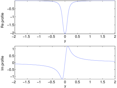
Figure 1: Re$\hat{\omega}^{RW}_{2}(\mathrm{i}y;15)$ and Im$\hat{\omega}^{RW}_{2}(\mathrm{i}y;15)$ profiles for the $\jmath=2$ frequency domain kernel $\hat{\omega}^{RW}_{2}(\mathrm{i}y;15)$. As indicated, $\ell=2$ and $\rho_{B}=15$.

$k$	Re$\beta^{RW}_{2,k}(15)$	Im$\beta^{RW}_{2,k}(15)$
1	$-$3.75616176922E$-$01	0
2	$-$2.52285897920E$-$01	0
3	$-$1.71458781191E$-$01	0
4	$-$1.16562490243E$-$01	0
5	$-$7.64331990276E$-$02	0
6	$-$4.68091057981E$-$02	0
7	$-$2.63730137927E$-$02	0
8	$-$1.25652994567E$-$02	0
9	$-$9.47795178947E$-$02	5.99312024947E$-$02
$k$	Re$\gamma^{RW}_{2,k}(15)$	Im$\gamma^{RW}_{2,k}(15)$
1	$-$9.42815440764E$-$06	0
2	$-$3.66046310052E$-$04	0
3	$-$3.74027383589E$-$03	0
4	$-$8.72734265927E$-$03	0
5	$-$1.47189136342E$-$03	0
6	$-$5.01356988668E$-$05	0
7	$-$9.73423621068E$-$07	0
8	$-$7.28807025058E$-$09	0
9	$-$8.94836172991E$-$02	6.20643548937E$-$02

Table 1: Compressed $\jmath=2$ Regge–Wheeler kernel for $\ell=2$, $\rho_{B}=15$, $\varepsilon=10^{-10}$. There are $d=10$ poles and strengths, and complex conjugation of the ninth entries gives the tenth entries. Zeros correspond to outputs from the compression algorithm which are less than $10^{-30}$ in absolute value.

$k$	Re$\beta^{Z}_{2,k}(15)$	Im$\beta^{Z}_{2,k}(15)$
1	$-$3.70827103177E$-$01	0
2	$-$2.48916278532E$-$01	0
3	$-$1.69097983283E$-$01	0
4	$-$1.14894340803E$-$01	0
5	$-$7.53169595130E$-$02	0
6	$-$4.61252633339E$-$02	0
7	$-$2.59880681276E$-$02	0
8	$-$1.23819599759E$-$02	0
9	$-$9.34065839850E$-$02	5.89802789971E$-$02
$k$	Re$\gamma^{Z}_{2,k}(15)$	Im$\gamma^{Z}_{2,k}(15)$
1	$-$8.94981130535E$-$06	0
2	$-$3.47903587670E$-$04	0
3	$-$3.56001528614E$-$03	0
4	$-$8.35011768248E$-$03	0
5	$-$1.41306545024E$-$03	0
6	$-$4.81777344134E$-$05	0
7	$-$9.35693850095E$-$07	0
8	$-$7.00652022551E$-$09	0
9	$-$8.70154844197E$-$02	6.01803999946E$-$02

Table 2: Compressed Zerilli kernel for $\ell=2$, $\rho_{B}=15$, $\varepsilon=10^{-10}$. There are $d=10$ poles and strengths, and complex conjugation of the ninth entries gives the tenth entries. Zeros correspond to outputs from the compression algorithm which are less than $10^{-30}$ in absolute value.

II.3 Kernel compression

With the ability to generate such numerical profiles for exact frequency–domain kernels, we have employed the technique of kernel compression in order to construct highly accurate numerical kernels which allow for efficient evaluation of the convolution appearing in (10). Introduced by AGH AGH and described further in both Jiang and Paper II, compression is vital both for high–$\ell$ kernels as well as low–$\ell$ kernels which are dominated by costly continuous sectors (such sectors are further described below). The technique produces a rational function,

$$\hat{\xi}_{\ell}(\sigma;\rho_{B})=\sum_{k=1}^{d}\frac{\gamma_{\ell,k}(\rho_{B})}{\sigma-\beta_{\ell,k}(\rho_{B})},$$ (11)

which approximates $\hat{\omega}_{\ell}(\sigma;\rho_{B})$ and is in fact a sum of $d$ simple poles. The pole locations $\beta_{\ell,k}(\rho_{B})$ and strengths $\gamma_{\ell,k}(\rho_{B})$ —output from the compression algorithm— lie in the lefthalf plane. The approximation is rigged to satisfy

$$\mathrm{sup}_{y\in R}\frac{\left|\hat{\xi}_{\ell}(\mathrm{i}y;\rho_{B})-\hat{\omega}_{\ell}(\mathrm{i}y;\rho_{B})\right|}{\left|\hat{\omega}_{\ell}(\mathrm{i}y;\rho_{B})\right|}<\varepsilon,$$ (12)

where $\varepsilon$ is a chosen numerical tolerance. Theoretically, this bound on the relative supremum error in the frequency domain ensures a long–time bound on the relative convolution error associated with (10), as discussed in AGH and Paper II. This convolution error arises when using the approximate time–domain kernel

$$\xi_{\ell}(\tau;\rho_{B})=\sum_{k=1}^{d}\gamma_{\ell,k}(\rho_{B})\exp\left[\beta_{\ell,k}(\rho_{B})\tau\right]$$ (13)

in place of the true kernel $\omega_{\ell}(\tau;\rho_{B})$. Since $\xi_{\ell}(\tau;\rho_{B})$ is a sum of exponentials, due to recursive identities an approximation of the convolution (10) based on $\xi_{\ell}(\tau;\rho_{B})$ is not memory intensive. We list representative compressed kernels for Regge–Wheeler and Zerilli kernels in Tables 1 and 2. The two kernels are strikingly similar, although they differ by a relative supremum error of about $3.03\times 10^{-2}$, well below their stated $\varepsilon=10^{-10}$ tolerances. Extensive numerical tables of compressed kernels are being prepared and will appear in LauEvans .

II.4 Quasinormal ringing and decay tail

Providing little detail, we now carry out a simple experiment meant only to indicate that the described ROBC work well for long–time simulations. More careful experiments were considered in Paper II (for Regge–Wheeler cases only) and will be considered in LauEvans . In terms of retarded time $\mu=\tau-\rho_{*}$ and the pulse function

$$g(\mu)=\left\{\begin{array}[]{rl}[\mu(\mu+4)]^{4}\big{/}256,&\quad\mathrm{for}-4\leq\mu\leq 0,\\ 0,&\quad\mathrm{otherwise},\end{array}\right.$$ (14)

we construct the $\ell=2$ wave packet

$$\Psi_{2}(0,\rho)=g(-\rho_{*})$$ (15)

as initial data for the Zerilli equation. The initial packet is then of unit height and compactly supported on $0\leq\rho_{*}\leq 4$. To complete the data, we assume that

$$\left.\left[\frac{\partial\Psi_{2}}{\partial\tau}+\frac{\partial\Psi_{2}}{\partial\rho_{*}}\right]\right|_{\tau=0}=0,$$ (16)

so that the pulse starts as essentially outgoing. We place the inner boundary at $\rho_{*}=-175$, and adopt (10) as the boundary condition at $\rho=\rho_{B}=15$, with an approximation of the exact ROBC based on the compressed kernel listed in the Table 2.

We evolve the data until $\tau=300$, using the MacCormack predictor–corrector algorithm. Throughout the evolution, we record the value $\Psi_{2}(\tau,3.25)$ of the field, that is to say, we record the history of the field in time at the fixed location $\rho=3.25$ (actually at the grid point nearest this location). Notice that the total run time is not long enough for the history $\Psi_{2}(\tau,3.25)$ to be influenced by reflection off of the inner boundary. The absolute value of the history is depicted as a linear–log plot in FIG. 2. It exhibits quasinormal ringing KokSchmidt until about $\tau=150$, and afterward a Price tail with the field decaying as $t^{-(2\ell+3)}=t^{-7}$ KokSchmidt . This late–time behavior stems from backscatter of the outgoing packet off of the long–range potential $V^{Z}(\rho)$. The dashed curve $3000t^{-7}$ has been eyeballed to fit the late–time decay tail.

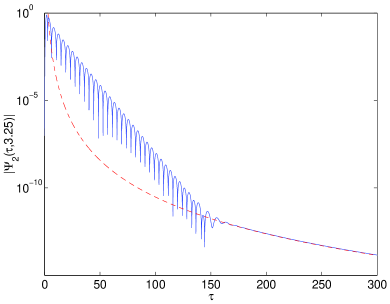
Figure 2: Quasinormal ringing and decay tail.

III Sum–of–poles representation

III.1 Flatspace FDNK and outgoing solution

AGH have considered nonreflecting boundary conditions (NRBC) for both 3+1 and 2+1 flatspace wave propagation, thoroughly treating both theoretical description and numerical approximation of NRBC for both scenarios AGH . For later comparison with the two gravitational scenarios, let us briefly recall the principal theoretical aspects of their work for the 3+1 scenario. To facilitate the comparison, we will use the same letters $\rho$, $\tau$, and $\sigma$ used for our dimensionless Schwarzschild coordinates, although for the flatspace case $r$, $t$, and $s$ would be more standard notations. Their boundary condition for a flatspace order–$\ell$ multipole $\Psi_{\ell}$ is

$$\left.\left(\frac{\partial\Psi_{\ell}}{\partial\tau}+\frac{\partial\Psi_{\ell}}{\partial\rho}\right)\right|_{\rho=\rho_{B}}=$$ (17)

$$\frac{1}{\rho_{B}}\int^{\tau}_{0}\omega^{F}_{\ell}(\tau-\tau^{\prime};\rho_{B})\Psi_{\ell}(\tau^{\prime},\rho_{B})\mathrm{d}\tau^{\prime},$$

comparable with (10). The exact TDRK $\omega^{F}_{\ell}(\tau;\rho_{B})$ appearing in (17) is now also a time–domain nonreflecting kernel (TDNK), and it is the inverse Laplace transform of an exact frequency–domain nonreflecting kernel (FDNK) admitting the following representation:AGH

$$\hat{\omega}^{F}_{\ell}(\sigma;\rho_{B})=\sum_{k=1}^{\ell}\frac{b_{\ell,k}/\rho_{B}}{\sigma-b_{\ell,k}/\rho_{B}},$$ (18)

where the $b_{\ell,k}$ are the zeros of the classical MacDonald function $K_{\ell+1/2}(z)$, a modified cylindrical Bessel function. Here the Bessel order is a half–integer, since we are considering the radial wave equation stemming from ordinary wave propagation on 3+1 flat spacetime, and these functions have the form Watson

$$K_{1/2}(z) = \sqrt{\frac{\pi}{2z}}e^{-z},$$

$$K_{3/2}(z) = \sqrt{\frac{\pi}{2z}}e^{-z}\left(1+\frac{1}{z}\right),$$

$$K_{5/2}(z) = \sqrt{\frac{\pi}{2z}}e^{-z}\left(1+\frac{3}{z}+\frac{3}{z^{2}}\right),$$

$$K_{7/2}(z) = \sqrt{\frac{\pi}{2z}}e^{-z}\left(1+\frac{6}{z}+\frac{15}{z^{2}}+\frac{15}{z^{3}}\right),$$ (19)

$$\vdots$$

$$K_{\ell+1/2}(z) = \sqrt{\frac{\pi z}{2}}(-1)^{\ell}z^{\ell}\left(\frac{1}{z}\frac{\mathrm{d}}{\mathrm{d}z}\right)^{\ell}\frac{e^{-z}}{z}.$$

The function $K_{\ell+1/2}(z)$ has $\ell$ simple zeros $\{b_{\ell,k}:k=1,\cdots,\ell\}$. When scaled by order, these zeros $(\ell+1/2)^{-1}b_{\ell,k}$ are known to accumulate on a fixed transcendental curve $\mathcal{C}$ in the lefthalf plane AGH ; Olver (the numerical methods developed in Paper I take advantage of this fact). Although this accumulation is asymptotic with large order $\ell+1/2\rightarrow\infty$, FIG. 3 shows that the agreement holds even for the lowest $\ell$, at least to the eye. The curve $\mathcal{C}$ shown in FIG. 3 has parametric form Olver ; Jiang

$$z(\lambda)=-\sqrt{\lambda^{2}-\lambda\tanh\lambda}\pm{\rm i}\sqrt{\lambda\coth\lambda-\lambda^{2}},$$ (20)

for $\lambda$ in the domain $[0,\lambda_{0}]$ with $\lambda_{0}\simeq 1.1997$ such that $\tanh\lambda_{0}=1/\lambda_{0}$. In terms of the “normalized–at–infinity” outgoing solution

$$W_{\ell}(z)=\sqrt{\frac{2z}{\pi}}\exp(z)K_{\ell+1/2}(z),$$ (21)

we have

$$\hat{\omega}^{F}_{\ell}(\sigma;\rho_{B})=\sigma\rho_{B}\frac{W_{\ell}^{\prime}(\sigma\rho_{B})}{W_{\ell}(\sigma\rho_{B})}$$ (22)

as another expression for the flatspace frequency–domain kernel AGH . In passing, we remark that although the exact FDNK (18) is already a rational function, the technique of kernel compression still proves useful for high–$\ell$ FDNK, since for a given tolerance $\varepsilon$ compression of (18) yields a numerical kernel with far fewer poles AGH .

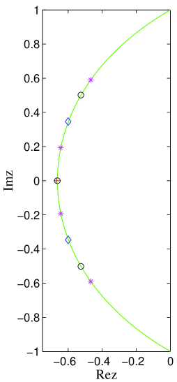
Figure 3: Scaled zeros of MacDonald functions. Here we plot scaled zeros $(\ell+1/2)^{-1}b_{\ell,k}$ for $\ell=1,2,3,4$. The cross is the scaled zero of $K_{1/2}(z)$, the diamonds are the scaled zeros of $K_{3/2}(z)$, the circles are the scaled zeros of $K_{5/2}(z)$, and the stars are the scaled zeros of $K_{7/2}(z)$.

III.2 Gravitational FDRK and outgoing solution

Let us first consider the relationship between a gravitational FDRK $\hat{\omega}_{\ell}(\sigma;\rho_{B})$ described earlier and solutions to the formal Laplace transform

$$\frac{\mathrm{d}^{2}\hat{\Psi}_{\ell}}{\mathrm{d}\rho_{*}^{2}}-V(\rho)\hat{\Psi}_{\ell}=\sigma^{2}\hat{\Psi}_{\ell}$$ (23)

of the generic equation (2). Here we mostly just collect relevant formulas. These formulas are derived in the first section of Paper I, and the derivation presented there goes through for Regge–Wheeler case ($\jmath=0,1,2$ considered there) as well as the Zerilli case (not considered there). Whence the formulas we consider now are valid for all cases.

We “peel off” the exponential behavior of the field by setting $\hat{\Psi}_{\ell}=\exp(-\sigma\rho_{*})\hat{\Phi}_{\ell}$, whereupon finding

$$\frac{\mathrm{d}^{2}\hat{\Phi}_{\ell}}{\mathrm{d}\rho^{2}}+\left(-2\sigma-\frac{1}{\rho}+\frac{1-2\sigma}{\rho-1}\right)\frac{\mathrm{d}\hat{\Phi}_{\ell}}{\mathrm{d}\rho}-\frac{\rho^{2}V(\rho)}{(\rho-1)^{2}}\hat{\Phi}_{\ell}=0$$ (24)

as the ODE satisfied by $\hat{\Phi}_{\ell}$. When numerically integrating (24) in various contexts, we have found it useful to work instead with $z=\sigma\rho$, re-expressing the equation as follows:

$$\frac{\mathrm{d}^{2}\hat{\Phi}_{\ell}}{\mathrm{d}z^{2}}+\left(-2-\frac{1}{z}+\frac{1-2\sigma}{z-\sigma}\right)\frac{\mathrm{d}\hat{\Phi}_{\ell}}{\mathrm{d}z}-\frac{z^{2}V(z/\sigma)}{\sigma^{2}(z-\sigma)^{2}}\hat{\Phi}_{\ell}=0.$$ (25)

Let $W_{\ell}(z;\sigma)$ denote the outgoing solution to (25). This solution obeys Olver

$$W_{\ell}(z;\sigma)\sim\sum_{k=0}^{\infty}d_{k}(\sigma)z^{-k}$$ (26)

as $z\rightarrow\infty$, and we describe it as “normalized at infinity.” Appendix B considers the recursion relations defining the $d^{RW}_{k}(\sigma)$ and $d^{Z}_{k}(\sigma)$. As described in Paper I, the flatspace solution $W_{\ell}(z)$ in (21) is formally $W_{\ell}(z)=W^{RW}_{\ell}(z;0)$ in terms of the Regge–Wheeler case $W^{RW}_{\ell}(z;\sigma)$.

In our notation $W_{\ell}(\sigma\rho;\sigma)$ is the outgoing solution to (24), and Paper I expresses the FDRK in terms of it as

$$\hat{\omega}_{\ell}(\sigma;\rho_{B})=\sigma\rho_{B}\frac{W^{\prime}_{\ell}(\sigma\rho_{B};\sigma)}{W_{\ell}(\sigma\rho_{B};\sigma)},$$ (27)

where the prime denotes differentiation in the first slot of $W_{\ell}(z;\sigma)$. Since we have peeled off the exponential factor $\exp(-\sigma\rho_{*})$ above and now work with an outgoing solution $W_{\ell}(\sigma\rho,\sigma)$ which is normalized at infinity, the FDRK (27) is more apt to have a well–defined inverse Laplace transform.

Paper I has described a collection of numerical methods which allow us to (i) evaluate $W_{\ell}(\sigma\rho_{B};\sigma)$ for $\sigma$ in the lefthalf plane and (ii) evaluate $\hat{\omega}_{\ell}(\mathrm{i}y;\rho_{B})$ for real $y$. We remark that Leaver has analytically represented a solution, say the outgoing one $W_{\ell}^{RW}(\sigma\rho_{B};\sigma)\exp(-\sigma\rho_{*})$, to the frequency–domain Regge–Wheeler equation as an infinite series in Coulomb wavefunctions, where the expansion coefficients obey a three–term recursion relation. In fact, such series expansions hold more generally for the generalized spheroidal wave equation (essentially the confluent Heun equation) Leaver . The methods described in Paper I are not based on the appropriate Leaver series, rather they rely on direct integration of (25). As such they can and have now been carried over to the Zerilli case. We note that the Zerilli equation is not directly related to the confluent Heun equation; whence it is not immediately evident how to evaluate $W^{Z}_{\ell}(\sigma\rho_{B};\sigma)$ via a Leaver series.

Roughly, our method for evaluating $W_{\ell}(\sigma\rho_{B};\sigma)$ is as follows. For a fixed frequency $\sigma$, initial data at a large radius are obtained for (25) using the asymptotic expansion (26). Then (25) is integrated over a suitable path in the complex $z=\sigma\rho$ plane to a terminal point $z_{B}=\sigma\rho_{B}$. To convey the basic idea behind our numerical evaluation of the FDRK $\hat{\omega}_{\ell}(\mathrm{i}y;\rho_{B})$ itself, we introduce

$$w_{\ell}(z;\sigma)=z\frac{W_{\ell}^{\prime}(z;\sigma)}{W_{\ell}(z;\sigma)}.$$ (28)

Then the FDRK is $\hat{\omega}_{\ell}(\sigma;\rho_{B})=w_{\ell}(\sigma\rho_{B};\sigma)$, and we have from (25) that $w_{\ell}(z;\sigma)$ obeys the first–order nonlinear equation

$$\frac{\mathrm{d}w_{\ell}}{\mathrm{d}z}+\frac{w^{2}_{\ell}}{z}+\left(-2-\frac{2}{z}+\frac{1-2\sigma}{z-\sigma}\right)w_{\ell}-\frac{z^{3}V(z/\sigma)}{\sigma^{2}(z-\sigma)^{2}}=0.$$ (29)

We calculate values $\hat{\omega}_{\ell}(\mathrm{i}y;\rho_{B})=w_{\ell}(\mathrm{i}y\rho_{B};\mathrm{i}y)$ via direct numerical integration of (29). To achieve stability and high accuracy, the methods associated with both (i) and (ii) evaluations require integration over nontrivial paths in the $z$–plane. Moreover, for technical reasons the integration employed for kernel evaluation (ii) is sometimes carried out in the complex $\rho$–plane rather than complex $z$–plane. Finally, we remark that to produce the origin value $\hat{\omega}_{\ell}(0;\rho_{B})$ of the kernel, we do not integrate (29). Rather, we make use of an exact series expression, one given for the Regge–Wheeler cases in Paper I and for the Zerilli case in Appendix A.

III.3 Gravitational sum–of–poles representation

For the case of $\jmath=0$ scalar perturbations Paper I has documented compelling numerical evidence indicating that the FDRK (27) admits an explicit “sum–of–poles” representation,

$$\hat{\omega}_{\ell}(\sigma;\rho_{B})=\sum_{k=1}^{N_{\ell}}\frac{\alpha_{\ell,k}(\rho_{B})}{\sigma-\sigma_{\ell,k}(\rho_{B})}-\frac{1}{\pi}\int^{\infty}_{0}\frac{f_{\ell}(\chi;\rho_{B})}{\sigma+\chi}\,{\rm d}\chi\,,$$ (30)

in terms of complex frequency $\sigma$. When we discussed compressed kernels before, we introduced approximate pole locations $\beta_{\ell,k}(\rho_{B})$ and strengths $\gamma_{\ell,k}(\rho_{B})$. We now consider $N_{\ell}$ (an integer) physical pole locations $\sigma_{\ell,k}(\rho_{B})$ and physical pole strengths $\alpha_{\ell,k}(\rho_{B})$, all of which lie in the lefthalf plane. Also appearing in (30) is a cut profile $f_{\ell}(\chi;\rho_{B})$, and like the pole locations and strengths it depends on the value of $\rho_{B}$. In principle the integer $N_{\ell}$ also depends $\rho_{B}$, but turns out to be constant over sizable regions of the relevant parameter space (more comments on this point below). The $k$th pole strength and cut profile are given respectively by

$$\alpha_{\ell,k}(\rho_{B})=-\rho_{B}\sigma_{\ell,k}^{\prime}(\rho_{B})\,,\quad f_{\ell}(\chi;\rho_{B})=\mathrm{Im}\hat{\omega}_{\ell}(\chi e^{{\rm i}\pi};\rho_{B})\,,$$ (31)

with $\chi\geq 0$ and the prime here standing for $\partial/\partial\rho_{B}$ differentiation.

We will argue that the representation (30) is also valid for both $\jmath=2$ Regge–Wheeler and Zerilli gravitational cases, and this conjecture is the main result of our paper. Note that (30) is not really a “sum of poles.” Indeed, recall that in the sense of complex analysis a pole is an isolated singularity. Strictly speaking then, the cut integral in (30) does not correspond to a “continuous distribution of poles” (an oxymoron). Nevertheless, we shall continue to describe the representation (30) as a “sum of poles.”

We stress that (30) is a representation for a boundary integral kernel. Its Laplace transform, the TDRK $\omega_{\ell}(\tau;\rho_{B})$, lives on the history of the spatial boundary $B$. Indeed, (10) makes no reference to the details of the initial data and is certainly not a spatial convolution over initial data. Moreover, the pole locations $\sigma_{\ell,k}(\rho_{B})$ are not quasinormal modes. An infinite number of quasinormal modes belong to each $\ell$ value, and these characteristic frequencies do not depend on any particular choice of outer boundary radius $\rho_{B}$. Quasinormal modes are associated with a boundary value problem specifying that $\hat{\Psi}_{\ell}$ is downgoing at the horizon and outgoing at infinity. The locations $\sigma_{\ell,k}(\rho_{B})$ are finite in number, and they do depend on $\rho_{B}$. They can be associated with a boundary value problem specifying that $\hat{\Psi}_{\ell}$ is outgoing at infinity and vanishes at $\rho_{B}$. Likewise, the cut integral appearing in (30) is not the branch–cut contribution to the usual Green’s function studied in the quasinormal mode problem Andersson .

IV Numerical study

In this section we both provide further qualitative description of the key representation (30) and justify it numerically. To argue that the representation (30) is valid for both $\jmath=2$ Regge–Wheeler and Zerilli gravitational cases, we offer nearly the same evidence as that offered in Paper I for the case of scalar perturbations. However, here we also consider one extra numerical experiment based on the Argument Principle. Our main numerical justification is to compare values $\hat{\omega}_{\ell}(\mathrm{i}y;\rho_{B})$ of the kernel obtain via two independent approaches. These are the following:

• Direct integration of (29) as alluded to above [a process which makes no use whatsoever of the conjecture representation (30)].

• Approximation of the sum–of–poles representation itself (by this we do not mean kernel compression).

In the second approach, we “build” the kernel as

$$\hat{\omega}_{\ell}(\mathrm{i}y;\rho_{B}) \simeq \sum_{k=1}^{N_{\ell}}\frac{\alpha_{\ell,k}(\rho_{B})+\delta\alpha_{\ell,k}(\rho_{B})}{\mathrm{i}y-\sigma_{\ell,k}(\rho_{B})-\delta\sigma_{\ell,k}(\rho_{B})}$$

$$-\frac{1}{\pi}\int^{\chi_{\mathrm{max}}}_{\chi_{\mathrm{min}}}\frac{f_{\ell}(\chi;\rho_{B})+\delta f_{\ell}(\chi;\rho_{B})}{\mathrm{i}y+\chi}\,{\rm d}\chi\,,$$

where the $\delta$ terms represent numerical errors and the integral over the chosen window $[\chi_{\mathrm{min}},\chi_{\mathrm{max}}]$ must be handled via numerical quadrature. We have used Simpson’s rule, respectively with 2048, 2048, 1024, 2048, 1024, 2048, 1024, 2048, 512 subintervals for $\ell=$ 2, 3, 4, 5, 6, 7, 8, 9, 10 (odd $\ell$ require more subintervals). We stress that this latter approach to evaluation, quite unlike the first approach, requires that we numerically compute all pole locations and strengths and well as the cut profile. To locate poles, zeros in $\sigma$ of $W_{\ell}(\sigma\rho_{B};\sigma)$, we have used the secant algorithm. The $\partial/\partial\rho_{B}$ derivatives of the $\sigma_{\ell,k}(\rho_{B})$ needed to compute the strengths $\alpha_{\ell,k}(\rho_{B})$ are obtained by first building a high–order interpolating polynomial $T_{\ell,k}(1/\rho_{B})$ for each $\sigma_{\ell,k}(\rho_{B})$ based on Chebyshev nodes in $1/\rho_{B}$. Derivatives are then found via differentiation of the Chebyshev polynomial. This procedure is described in more detail in Paper I where it was used for the $\jmath=0$ Regge–Wheeler case.

We remark that this direct approximation (IV) to the sum–of–poles representation (30) is certainly not a compressed kernel. Indeed, as mentioned, this brute–force approximation of (30) typically requires thousands of poles (stemming from the numerical quadrature of the cut integral) to achieve the same error tolerance achieved by a compressed kernel comprised of ten or so poles.

Besides making the comparison outlined in the last paragraph, we also wish to provide further qualitative description of the sum–of–poles representation (30). We describe both the poles and the cut profile in more detail, and also compare the representation to the strikingly similar representation (18) of the FDNK $\hat{\omega}^{F}_{\ell}(\sigma;\rho_{B})$ for a flatspace order–$\ell$ multipole. We have found that both gravitational kernels, $\hat{\omega}^{RW}_{\ell}(\sigma;\rho_{B})$ and $\hat{\omega}^{Z}_{\ell}(\sigma;\rho_{B})$, indeed agree with $\hat{\omega}^{F}_{\ell}(\sigma;\rho_{B})$ in the $\rho_{B}\rightarrow\infty$ limit, although here we will focus on the Zerilli case. One certainly expects such agreement, since the Schwarzschild solution is asymptotically flat. However, the nature of this asymptotic agreement is rather interesting, and we point out some subtleties not mentioned in Paper I.

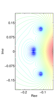
Figure 4: Zeros $\{\sigma^{Z}_{3,k}(15):1\leq k\leq 4\}$ in frequency of $W_{3}^{Z}(\sigma 15;\sigma)$. The contour lines are of $\log_{10}|W_{3}^{Z}(\sigma 15;\sigma)|$, with the logarithm distributing contour lines more evenly.

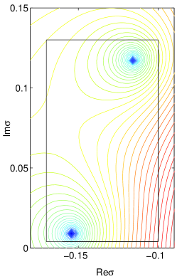
Figure 5: Zeros in frequency of $W_{3}^{Z}(\sigma 15;\sigma)$. The plot here is a blow–up of the one shown in FIG. 4.

IV.1 Pole locations and strengths

For the most part, this subsection gives what amounts to a qualitative description. Using our method for evaluating the outgoing solution $W_{\ell}(\sigma\rho_{B};\sigma)$, we may plot the modulus $|W_{\ell}(\sigma\rho_{B};\sigma)|$ in order to suggest rough values for zeros (that is, roots) of the function. Provided such a zero is simple, it will correspond to a pole appearing in the representation (30). Over the parameter space $\rho_{B}\geq 15$ and $\ell=2,3,\cdots 10$, and for both Zerilli and $\jmath=2$ Regge–Wheeler cases, we have found that the number $N_{\ell}$ of zeros $\sigma_{\ell,k}(\rho_{B})$ is as follows: $N_{2}=2$, $N_{3}=4=N_{4}$, $N_{5}=6=N_{6}$, $N_{7}=8=N_{8}$, $N_{9}=10=N_{10}$. For a fixed choice of $\ell$ and $\rho_{B}$, these zeros form a crescent pattern in the lefthalf $\sigma$–plane.

For example, FIG. 4 depicts the modulus $|W_{3}^{Z}(\sigma 15;\sigma)|$ in the indicated region of the lefthalf $\sigma$ plane. Four zeros appear to be evident in the figure, and in order to further explore whether or not they are indeed zeros, we appeal to the Argument Principle. We focus on the two upper locations shown closer up in FIG. 5. Let $h(\sigma)=W^{Z}_{3}(\sigma 15;\sigma)$ represent our numerically computed function. We numerically compute

$$\frac{1}{2\pi\mathrm{i}}\oint_{\mathrm{square}}\frac{h^{\prime}(\sigma)}{h(\sigma)}\mathrm{d}\sigma\simeq 1.999732-\mathrm{i}4.185506\times 10^{-5}$$ (33)

over the square (running in the counterclockwise sense) shown in FIG. 5. On each side of the square we have introduced 1024 subintervals, and used the trapezoid rule. Since we are unable to numerically evaluate $h^{\prime}(\sigma)$ directly, we approximate this derivative using difference quotients (this requires two extra function evaluations beyond the corners). Using a sequence of discretizations, we have confirmed that the integral convergences to $2$ at a second–order rate, suggesting that the square indeed encloses two simple zeros. As a second example, consider the modulus $|W_{8}^{Z}(\sigma 25;\sigma)|$ plotted in FIG. 6 over the indicated region (four other zeros, conjugate to those shown, are located in the third quadrant). For the analogous line–integral over the square shown (and using 2048 cells on each side for the trapezoidal integration), we find a value of $3.999975-\mathrm{i}5.169761\times 10^{-5}$, suggesting four simple zeros.

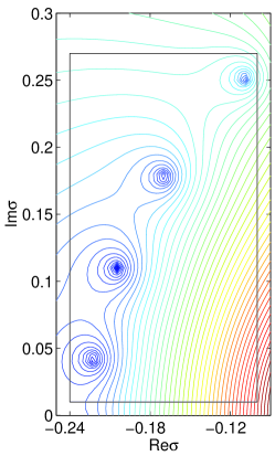
Figure 6: Zeros in frequency of $W_{8}^{Z}(\sigma 25;\sigma)$. The contour lines are of $\log_{10}|W_{8}^{Z}(\sigma 25;\sigma)|$, with the logarithm distributing contour lines more evenly.

As with the scalar case, we find for the Zerilli and $\jmath=2$ Regge–Wheeler cases that the zeros $\sigma_{\ell,k}(\rho_{B})$ in frequency of $W_{\ell}(\sigma\rho_{B};\sigma)$ behave asymptotically as

$$\sigma_{\ell,k}(\rho_{B})\sim b_{\ell,k}/\rho_{B}$$ (34)

in the $\rho_{B}\rightarrow\infty$ limit. However, let us offer several important observations in order to sharpen the precise nature of this asymptotic agreement. First, in the opposite limit as $\rho_{B}\rightarrow 1^{+}$, we do not believe $N_{\ell}$ remains constant. Indeed, we expect the phenomenon of “zero pair creation” in this limit, as described in Paper I for the scalar $\jmath=0$ Regge–Wheeler FDRK. Although we believe that the sum–of–poles representation remains valid for $\rho_{B}$ close (but not equal) to unity, description of the FDRK and implementation of ROBC both become more difficult in this limit. For these reasons, we have required $\rho_{B}\geq 15$. Second, for odd $\ell$ there is an “extra” zero. That is to say, for odd $\ell$ the number $N_{\ell}=\ell+1$ of zeros $\sigma_{\ell,k}(\rho_{B})$ is greater by one than the number $\ell$ of MacDonald zeros (provided $\rho_{B}$ is large enough, otherwise $N_{\ell}$ could be a larger integer still). We will argue that this curious feature is not at odds with the asymptotic result (34) above. Let us focus on the Zerilli case, with the understanding that similar statements apply to the $\jmath=2$ Regge–Wheeler case.

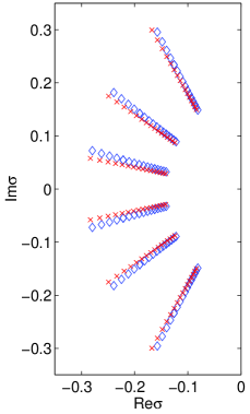
Figure 7: Zeros $\{\sigma^{Z}_{6,k}(\rho_{B}):1\leq k\leq 6\}$ in frequency of $W_{6}^{Z}(\sigma\rho_{B};\sigma)$. Diamonds represent the zeros $\sigma_{6,k}(\rho_{B})$, while the crosses represent the $b_{6,k}/\rho_{B}$. All zeros for $\rho_{B}=15,16,\cdots,30$ are shown. The outermost crescent of locations corresponds to $\rho_{B}=15$ and the innermost to $\rho_{B}=30$.

For even $\ell=2,4,6,8,10$ and $\rho_{B}\geq 15$, the number of zeros $\sigma^{Z}_{\ell,k}(\rho_{B})$ is $N_{\ell}=\ell$, the same as the number of $b_{\ell,k}/\rho_{B}$. As an illustration, FIG. 7 depicts the six zeros $\sigma^{Z}_{6,k}(\rho_{B})$ of $W_{6}^{Z}(\sigma\rho_{B};\sigma)$ as diamonds for $\rho_{B}=15,16,\cdots,30$. We also plot the corresponding MacDonald–Bessel zeros $b_{6,k}/\rho_{B}$ as crosses. The collection $\sigma^{Z}_{6,k}(15)$ of zeros is the outermost crescent of diamonds, while the collection $\sigma^{Z}_{6,k}(30)$ is the innermost (and similarly for the crescents of Bessel crosses). The plot is clearly not at odds with the asymptotic formula (34) above.

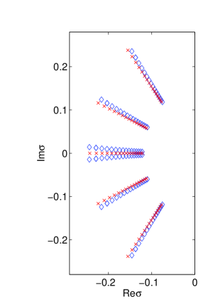
Figure 8: Zeros $\{\sigma^{Z}_{5,k}(\rho_{B}):1\leq k\leq 6\}$ in frequency of $W_{5}^{Z}(\sigma\rho_{B};\sigma)$. Diamonds represent the zeros $\sigma^{Z}_{5,k}(\rho_{B})$, while the crosses represent $b_{5,k}/\rho_{B}$. All zeros for $\rho_{B}=15,16,\cdots,30$ are shown. The outermost crescent of locations corresponds to $\rho_{B}=15$ and the innermost to $\rho_{B}=30$. For each $\rho_{B}$ two diamonds correspond to the single cross lying on the negative real axis.

As mentioned, for odd $\ell=1,3,5,7,9$ and $\rho_{B}\geq 15$, the number of zeros $\sigma^{Z}_{\ell,k}(\rho_{B})$ is $N_{\ell}=\ell+1$, that is one more than the corresponding number of MacDonald–Bessel zeros. For odd $\ell$ there is a single MacDonald–Bessel zero which lies on negative real axis. As with the $\jmath=0$ Regge–Wheeler case, we find for odd $\ell$ that two zeros of $W^{Z}_{\ell}(\sigma\rho_{B};\sigma)$ correspond to this single real MacDonald–Bessel zero. Moreover, as $\rho_{B}$ gets large each of these two zeros is asymptotic to the single MacDonald–Bessel zero. This phenomenon is evident in FIG. 8, and corresponding plots for other odd $\ell$ are similar. The existence of an “extra” zero is at first sight troubling in light of the expected asymptotic agreement between $\hat{\omega}^{Z}_{\ell}(\mathrm{i}y;\rho_{B})$ and $\hat{\omega}^{F}_{\ell}(\mathrm{i}y;\rho_{B})$. However, we argue below that the pole and cut contributions to the gravitational FDRK in tandem do yield the correct asymptotic agreement.

So far we have only consider locations $\sigma^{Z}_{\ell,k}(\rho_{B})$ associated with Zerilli kernels. To the eye, both FIGS. 7 and 8 would be the same had we instead plotted the corresponding locations $\sigma^{RW}_{\ell,k}(\rho_{B})$ associated with $\jmath=2$ Regge–Wheeler kernels. For the examples we have considered, $|\sigma^{Z}_{\ell,k}(\rho_{B})-\sigma^{RW}_{\ell,k}(\rho_{B})|$ is typically on the order of $10^{-5}$ to $10^{-3}$. However, from Paper I results we know that this difference is seven to ten orders of magnitude larger than our knowledge of these locations. As an example, we list the two conjugate locations $\sigma_{2,k}(15)$ for $\jmath=0$ Regge–Wheeler, $\jmath=2$ Regge–Wheeler, and Zerilli cases. Respectively, these are
$-0.096885391711329\pm\mathrm{i}0.061245961499841$,
$-0.094779501145744\pm\mathrm{i}0.059927941363806$,
$-0.093406539086840\pm\mathrm{i}0.058977077340679$.
These locations are all quite similar, and they may be compared to the roots $b_{2,k}/15$: $-(3/2\pm\mathrm{i}\sqrt{3}/2)/15=-0.1\pm\mathrm{i}0.05773502691896$. In this short list the last location, say, clearly corresponds in some sense to the ninth pole location in the compressed kernel in Table 2, but note that the absolute difference between the value here and the table value is more than the stated $\varepsilon=10^{-10}$ tolerance for the compressed kernel. See the footnote just after Eq. (30).

IV.2 Cut profile

Using the type (i) numerical method from Paper I described above [which also returns derivative information for $W_{\ell}^{\prime}(\sigma\rho_{B};\sigma)$], we have generated Zerilli cut profiles $f^{Z}_{\ell}(\chi;\rho_{B})$ for various $\ell$ and $\rho_{B}$. FIG. 9 depicts profiles for even $\ell$. To the eye the cut profiles shown match $\jmath=2$ Regge–Wheeler profiles $f^{RW}_{\ell}(\chi;\rho_{B})$ corresponding to the same parameter choices. However, the Zerilli and Regge–Wheeler even profiles are indeed different, as is shown by an example plot in FIG. 11. Near the peak of this plotted difference, the accuracy to which we know the Zerilli and Regge–Wheeler profiles is some ten orders of magnitude greater than the difference. Notice that these even cut profiles weaken as $\rho_{B}$ gets larger, and we believe that the cut contribution to an even–$\ell$ gravitational FDRK “dies out” as $\rho_{B}$ gets large. Based on our earlier claim that for an even–$\ell$ gravitational FDRK we have the same number $N_{\ell}=\ell$ of zeros $\sigma_{\ell,k}(\rho_{B})$ as Bessel zeros $b_{\ell,k}/\rho_{B}$, and that these zeros lock on to the latter as $\rho_{B}$ gets large, we conjecture that the even–$\ell$ kernels $\hat{\omega}^{Z}_{\ell}(\mathrm{i}y;\rho_{B})$ and $\hat{\omega}^{RW}_{\ell}(\mathrm{i}y;\rho_{B})$ both approach $\hat{\omega}^{F}_{\ell}(\mathrm{i}y;\rho_{B})$ uniformly in $y$ as $\rho_{B}\rightarrow\infty$.

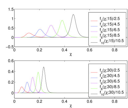
Figure 9: Scaled even cut profiles for Zerilli kernels. In each plot the leftmost profile is $f^{Z}_{2}(\chi;\rho_{B})\big{/}2.5$ and the rightmost $f^{Z}_{10}(\chi;\rho_{B})\big{/}10.5$.

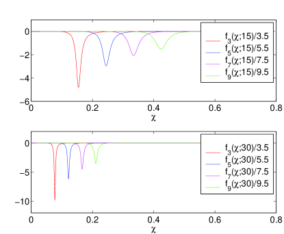
Figure 10: Scaled odd cut profiles for Zerilli kernels. In each plot the leftmost profile is $f^{Z}_{3}(\chi;\rho_{B})\big{/}3.5$ and the rightmost $f^{Z}_{9}(\chi;\rho_{B})\big{/}9.5$.

We plot odd–$\ell$ Zerilli cut profiles in FIG. 10. Like before with the even–$\ell$ profiles, to the eye these could be either Zerilli or $\jmath=2$ Regge–Wheeler profiles. However, as is evident in the bottom plot shown in FIG. 11, these cases are different. Notice that for odd $\ell$ the cut profiles strengthen as $\rho_{B}$ increases. We believe that such a strengthening profile in tandem with the two zeros closest to the real axis as a whole combine to asymptotically agree with the single MacDonald–Bessel zero $b_{\ell,0}/\rho_{B}$ located on the negative real axis. [For notational simplicity we have now labeled this zero by $k=0$. Before it would have corresponded to $k=\frac{1}{2}(\ell+1)$ for odd $\ell$, if $k=1,\cdots,\ell$ for the zeros $b_{\ell,k}$ of $K_{\ell+1/2}(z)$.] In other words, for odd–$\ell$ the cut profile in effect cancels one of the zeros $\sigma_{\ell,k}(\rho_{B})$, so that we again we have agreement between the gravitational FDRK $\hat{\omega}^{Z}_{\ell}(\mathrm{i}y;\rho_{B})$ and flatspace FDNK $\hat{\omega}^{F}_{\ell}(\mathrm{i}y;\rho_{B})$ uniformly in $y$ as $\rho_{B}\rightarrow\infty$. While we cannot precisely describe how this cancellation of the extra zero occurs, we believe that it stems from the following two conjectures, claimed to hold as $\rho_{B}\rightarrow\infty$. First, the cut profile becomes sharply concentrated for $\chi$ near $-b_{\ell,0}/\rho_{B}$. Second,

$$-\frac{1}{\pi}\int_{0}^{\infty}f_{\ell}(\chi;\rho_{B})\mathrm{d}\chi\sim-b_{\ell,0}/\rho_{B}.$$ (35)

Preliminary numerical investigations indicate that both claims are in fact valid, but the issue deserves further study (preferably theoretical). All statements made in this paragraph also pertain to $\hat{\omega}^{RW}_{\ell}(\mathrm{i}y;\rho_{B})$.

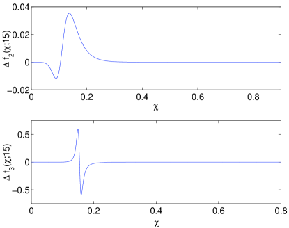
Figure 11: Difference between Regge–Wheeler and Zerilli cut profiles. Here we plot example differences with the notation $\Delta f_{\ell}(\chi;15)=f^{RW}_{\ell}(\chi;15)-f^{Z}_{\ell}(\chi;15)$.

IV.3 Numerical validation of the sum–of–pole representation

Up to this point we have mainly given a qualitative description of what we believe are the main features of the sum–of–poles representation (30). In order to quantitatively test our representation (30), we compare the two numerical approaches for evaluating either $\hat{\omega}^{Z}_{\ell}(\mathrm{i}y;\rho_{B})$ or $\hat{\omega}^{RW}_{\ell}(\mathrm{i}y;\rho_{B})$ outlined at the beginning of this section. FIG. 12 depicts such a comparison for the Zerilli case with $\ell=2$ and $\rho_{B}=15$. To make the plots in the figure, we have used a $y$–grid with 5 adaptive levels, each with 32 grid points. The adaptive grid provides more resolution near the origin where we expect the largest errors. We have then generated two separate numerical arrays of values $\hat{\omega}^{Z}_{2}(\mathrm{i}y;15)$ on the $y$–grid, the first obtained by integrating the ODE (29) and the second via the direct construction (IV). Both arrays of numerical values are obtained in double precision arithmetic. The plots depict the absolute error $|\Delta\hat{\omega}^{Z}_{2}(\mathrm{i}y;15)|$ and relative error $|\Delta\hat{\omega}^{Z}_{2}(\mathrm{i}y;15)|\big{/}|\hat{\omega}^{Z}_{2}(\mathrm{i}y;15)|$ over the $y$–grid, and they indicate striking agreement between the two methods. We note that the maximum value of the absolute error in the top plot is $1.49\times 10^{-12}$, and the maximum value of the relative error in the bottom plot is $7.35\times 10^{-13}$. We can now perform the same experiment over a range of $\rho_{B}$ values, say $\rho_{B}=15,16,\cdots,30$. For each choice of $\rho_{B}$ we compute maximum values of absolute and relative error over the $y$–grid. It turns out that the same values above corresponding to $\rho_{B}=15$ are the largest errors encountered.

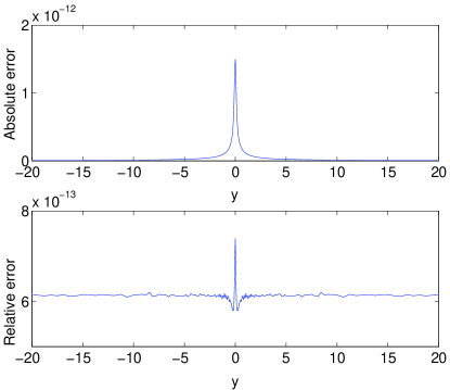
Figure 12: Relative and absolute numerical errors. Here we plot numerical errors corresponding to $|\Delta\hat{\omega}^{Z}_{2}(\mathrm{i}y;15)|$ and $|\Delta\hat{\omega}^{Z}_{2}(\mathrm{i}y;15)|\big{/}|\hat{\omega}^{Z}_{2}(\mathrm{i}y;15)|$ for the Zerilli case with $\ell=2$ and $\rho_{B}=15$.

We now perform the same experiment for each $\ell\leq 10$ and for both $\jmath=2$ Regge–Wheeler and Zerilli cases. That is to say, for each $\ell$ we compute the maximum absolute error $|\Delta\hat{\omega}_{\ell}(\mathrm{i}y;\rho_{B})|$ and maximum relative error $|\Delta\hat{\omega}_{\ell}(\mathrm{i}y;\rho_{B})|\big{/}|\hat{\omega}_{\ell}(\mathrm{i}y;\rho_{B})|$ uniformly over the described $y$–grid and all $\rho_{B}=15,16,\cdots,30$. For the Zerilli case we list these errors in the Table 3. Errors for the $\jmath=2$ Regge–Wheeler case are comparable.

$\ell$	Max relative error	Max absolute error
2	$7.35\times 10^{-13}$	$1.49\times 10^{-12}$
3	$3.63\times 10^{-12}$	$9.50\times 10^{-12}$
4	$8.63\times 10^{-13}$	$2.47\times 10^{-12}$
5	$1.27\times 10^{-12}$	$4.68\times 10^{-12}$
6	$6.17\times 10^{-13}$	$2.15\times 10^{-12}$
7	$6.93\times 10^{-13}$	$4.69\times 10^{-12}$
8	$3.03\times 10^{-13}$	$1.51\times 10^{-12}$
9	$5.10\times 10^{-13}$	$3.51\times 10^{-12}$
10	$9.71\times 10^{-14}$	$8.92\times 10^{-13}$

Table 3: Zerilli errors

V Conclusion

For both flatspace 3+1 and flatspace 2+1 wave propagation and nonreflecting boundary conditions, AGH proved several theorems related to both the exact sum–of–poles representation for a FDNK (also a FDRK, but we have used FDNK for the special flatspace case) and its numerical approximation AGH . In particular, they proved that a FDNK admits a rational approximation as a compressed kernel, and for a given large Bessel order $\nu$ (for the 3+1 case $\nu=\ell+1/2$) and choice of $\varepsilon$ tolerance they estimated the required number $d$ of poles appearing in the compressed kernel. In addition to some techniques stemming from the Fast Multipole Method, their proofs rely heavily on the well–understood theory of Bessel functions. In particular, AGH made extensive use of integral representations, order recursion relations, and detailed understanding of the scaling behavior for both the poles and (for the 2+1 case) the cut profile.

While the numerical evidenced amassed here is extremely convincing, it does not constitute a mathematical proof that a gravitational FDRK admits the representation (30), and we hope that our numerical investigation spurs the interest of analysts capable of theoretically investigating our conjectured representation. Were (30) established theoretically, we believe approximation theorems —similar to those proved by AGH but pertaining to our gravitational ROBC— would follow. One might prove that a gravitational FDRK also admits a rational approximation as a compressed kernel, and determine the asymptotic growth of the number $d$ of approximating poles as $\ell\rightarrow\infty$, $\varepsilon\rightarrow 0^{+}$. Since numerically constructed compressed kernels have performed spectacularly in implementations of ROBC (see Paper II), we have good reason to believe that approximation theorems must hold. Such theorems are bound to involve the details of the underlying special functions. Unfortunately, relative to Bessel functions, significantly less is known about the special functions considered here, confluent Heun functions for the Regge–Wheeler cases and seemingly more exotic functions for the Zerilli case. Indeed, we are unaware of useful integral representations, and while appropriate Leaver series are certainly of formal interest, they would not seem a good platform for carrying out the requisite asymptotic analysis. While our own knowledge of modern analysis would seem not up to such theoretical investigation, we believe our results offer fertile new ground for more capable analysts.

VI Acknowledgments

I thank C. R. Evans, C. O. Lousto, and R. H. Price for clarifying remarks about blackhole perturbation theory, and gratefully acknowledge support from NSF grant PHY0514282.

Appendix A Origin value of the FDRK

For the $\jmath=0,1,2$ Regge–Wheeler cases Paper I has expressed the origin value $\hat{\omega}^{RW}_{\ell}(0;\rho_{B})$ of the FDRK in terms of an infinite series in $\rho^{-1}_{B}$, where the expansion coefficients obey a two–term recursion relation (see Section 3.2.3 of that reference). All expansion coefficients are positive, and the value $\hat{\omega}^{RW}_{\ell}(0;\rho_{B})$ can be accurately approximated in terms of two partial sums. This series was used numerically to evaluate the kernel at the origin $\sigma=0$, a frequency value for which direct integration of (29) proved problematic.

To express $\hat{\omega}^{Z}_{\ell}(0;\rho_{B})$ for the Zerilli case of polar perturbations, we have used a similar series expression, although now the series coefficients obey a four–term rather than two–term recursion relation. We have obtained this series via the following recipe. First, we set $\sigma=0$ in (24) and use (LABEL:Zerpotential), thereby reaching

$$\frac{\mathrm{d}^{2}\hat{\Phi}_{\ell}}{\mathrm{d}\rho^{2}}+\left(-\frac{1}{\rho}+\frac{1}{\rho-1}\right)\frac{\mathrm{d}\hat{\Phi}_{\ell}}{\mathrm{d}\rho}$$ (36)

$$-\left[\frac{8n^{2}(n+1)\rho^{3}+12n^{2}+18n\rho+9}{\rho^{2}(\rho-1)(2n\rho+3)^{2}}\right]\hat{\Phi}_{\ell}=0.$$

Next, plugging the expansion

$$\hat{\Phi}_{\ell}=\sum_{k=0}^{\infty}a_{k}\rho^{-(\ell+k)}$$ (37)

into (36), assuming $a_{0}=1$, and balancing terms, we find the recursion relation

$$\beta_{k}a_{k+3}+\gamma_{k}a_{k+2}+\delta_{k}a_{k+1}+\epsilon_{k}a_{k}=0,$$ (38)

where

$$\beta_{k} = 4n^{2}[(\ell+k+3)(\ell+k+4)-2(n+1)],$$

$$\gamma_{k} = 4n(\ell+k+2)[(3-n)(\ell+k+3)-n]-12n^{2},$$

$$\delta_{k} = (\ell+k+1)[(9-12n)(\ell+k+2)-12n]-18n,$$

$$\epsilon_{k} = -9(\ell+k+1)^{2}.$$ (39)

Again $n=\frac{1}{2}(\ell-1)(\ell+2)$, and in the start–up, $\delta_{-2}=0=\epsilon_{-2}$ and $\epsilon_{-1}=0$. The origin value of the FDRK is

$$\hat{\omega}^{Z}_{\ell}(0;\rho_{B})=\left.-\sum_{k=0}^{\infty}(\ell+k)a_{k}\rho_{B}^{-(\ell+k)}\right/\sum_{k=0}^{\infty}a_{k}\rho_{B}^{-(\ell+k)}.$$ (40)

Despite the four–term recursion relation used to generate the series and its $\rho$–derivative, in using (40) we have encountered no numerical instabilities.

Appendix B Asymptotic expansion for outgoing solution

To generate initial data for our numerical methods based on path integration in the complex $z$–plane (or sometimes the complex $\rho$–plane), we use the asymptotic expansion (26) about the irregular singular point at infinity. Paper I describes this expansion for all the Regge–Wheeler cases, showing that the $d^{RW}_{k}(\sigma)$ obey a three–term recursion relation. For the Zerilli case, we write the expansion coefficients as $d^{Z}_{k}(\sigma)=g_{k}(\sigma)\sigma^{k}$, then finding that the $g_{k}(\sigma)$ obey the five–term recursion relation

$$A_{k}g_{k+4}+B_{k}g_{k+3}+C_{k}g_{k+2}+D_{k}g_{k+1}+E_{k}g_{k}=0,$$ (41)

where

$$A_{k} = 8\sigma n^{2}(k+4),$$

$$B_{k} = 4n(k+3)[6\sigma+n(k+4)]-8n^{2}(n+1)$$

$$C_{k} = (k+2)[18\sigma-4n^{2}+(12n-4n^{2})(k+3)]-12n^{2}$$

$$D_{k} = (k+1)[(9-12n)(k+2)-12n]-18n$$

$$E_{k} = -9(k+1)^{2}.$$ (42)

Here again $n=\frac{1}{2}(\ell-1)(\ell+2)$, and in the start–up $C_{-3}=D_{-3}=E_{-3}=0$, $D_{-2}=E_{-2}=0$, and $E_{-1}=0$. Typically, we have used fewer than ten terms in the expansion (26) to generate initial data for numerical integration, and have encountered no problems in using this expansion (despite potentially tricky issues associated with high–order recursions). We have used dimensionless coordinates and Laplace rather than Fourier transform. Adjusting for these choices, (41) and (42) agree with an expansion given by Chandrasekhar and Detweiler in ChandraDet2 .

References

- (1) J. A. Wheeler, Phys. Rev. 97, (1955) 511.
- (2) T. Regge and J. A. Wheeler, Phys. Rev. 108, (1957) 1063.
- (3) F. J. Zerilli, Phys. Rev. D 2, (1970) 2141.
- (4) R. H. Price, Phys. Rev. D 5, (1972) 2439.
- (5) S. Chandrasekhar, Mathematical Theory of Black Holes, (Oxford University Press, Oxford, 1992).
- (6) A. Anderson and R. Price, Phys. Rev. D 43, (1991) 3147–3154.
- (7) R. H. Price and J. Pullin, Phys. Rev. Lett. 72 (1994) 3297.
- (8) H.–P. Nollert, J. Baker, R. Price, and J. Pullin, in Proceedings of the 18th Texas Symposium on Relativistic Astrophysics, gr-qc/9710011.
- (9) R. Gleiser, O. Nicasio, R. Price, and J. Pullin, Phys. Rev. Lett. 77 (1996) 4483.
- (10) R. Gleiser, O. Nicasio, R. Price, and J. Pullin, Phys. Rev. D 59 (1999) 044024.
- (11) C. O. Lousto, Phys. Rev. Lett. 84 (2000) 5251.
- (12) C. O. Lousto, A fourth order convergent numerical algorithm to integrate nonrotating binary black hole perturbations in the extreme mass ratio limit, gr-qc/0503001.
- (13) See http://math.ucr.edu/home/baez/area.html for a detailed literature review of this issue.
- (14) O. Dreyer, Phys. Rev. Lett. 90 (2003) 081301; Contribution to the Proceedings of the 3rd International Symposium on Quantum Theory and Symmetries, Cincinnati, September 2003, gr-qc/0404055.
- (15) M. Domagala and J. Lewandowski, Class. Quantum Grav. 21 (2004) 5233.
- (16) L. Motl and A. Neitzke, Adv. Theor. Math. Phys. 7 (2003) 307.
- (17) S. Musiri and G. Siopsis, Class. Quant. Grav. 20 (2003) L285.
- (18) J. W. York, Jr. and B. S. Schmekel, Phys. Rev. D 72, (2005) 024022.
- (19) J. W. York, Jr., Phys. Rev. D 28 (1983) 2929.
- (20) B. Alpert, L. Greengard, and T. Hagstrom, SIAM J. Numer. Anal. 37 (2000) 1138.
- (21) S. R. Lau, J. Comput. Phys. 199 (2004) 376.
- (22) S. R. Lau, Class. and Quantum Grav 21 (2004) 4147.
- (23) C. R. Evans and S. R. Lau, The tail of the outer boundary, in preparation, Summer and Fall 2005.
- (24) K. D. Kokkotas and B. G. Schmidt, “Quasi–Normal Modes of Stars and Black Holes,” Living Reviews of Relativity 2, 2, and gr–qc/9909058.
- (25) Heun’s Differential Equations, edited by A. Ronveaux (Oxford University Press, Oxford, 1995).
- (26) S. Y. Slavyanov and W. Lay, Special Functions: a Unified Theory Based on Singularities (Oxford University Press, Oxford, 2000).
- (27) R. J. LeVeque, Numerical Methods for Conservation Laws, second edition (Birkhäuser Verlag, Basel, 1992).
- (28) Olver, F. W. J. Asymptotics and Special Functions (Academic Press, New York and London, 1974).
- (29) E. W. Leaver, J. Math. Phys. 27 (1986) 1238.
- (30) H.–P. Nollert and B. G. Schmidt, Phys. Rev. D 45 (1992) 2617.
- (31) See, for example, N. Andersson, Phys. Rev. D 55 (1997) 468.
- (32) G. N. Watson, A Treatise on the Theory of Bessel Functions, second edition (Cambridge University Press, Cambridge, 1944).
- (33) S. Jiang, Fast Evaluation of Nonreflecting Boundary Conditions for the Schrödinger Equation, New York University Ph.D. Dissertation (2001).
- (34) S. Chandrasekhar and S. Detweiler, Proc. R. Soc. Lond. A 344 (1975) 441.