Search for gravitational waves from galactic and extra–galactic binary neutron stars}

Abstract

We use 373 hours ($\approx$ 15 days) of data from the second science run of the LIGO gravitational-wave detectors to search for signals from binary neutron star coalescences within a maximum distance of about 1.5 Mpc, a volume of space which includes the Andromeda Galaxy and other galaxies of the Local Group of galaxies. This analysis requires a signal to be found in data from detectors at the two LIGO sites, according to a set of coincidence criteria. The background (accidental coincidence rate) is determined from the data and is used to judge the significance of event candidates. No inspiral gravitational wave events were identified in our search. Using a population model which includes the Local Group, we establish an upper limit of less than $47$ inspiral events per year per Milky Way equivalent galaxy with 90% confidence for non-spinning binary neutron star systems with component masses between 1 and 3 $M_{\odot}$.

Currently at ]Stanford Linear Accelerator Center Currently at ]Jet Propulsion Laboratory Permanent Address: ]HP Laboratories Currently at ]Rutherford Appleton Laboratory Currently at ]University of California, Los Angeles Currently at ]Hofstra University Permanent Address: ]GReCO, Institut d’Astrophysique de Paris (CNRS) Currently at ]Jet Propulsion Laboratory Currently at ]La Trobe University, Bundoora VIC, Australia Currently at ]Keck Graduate Institute Currently at ]National Science Foundation Currently at ]University of Sheffield Currently at ]Ball Aerospace Corporation Currently at ]Jet Propulsion Laboratory Currently at ]European Gravitational Observatory Currently at ]Intel Corp. Currently at ]University of Tours, France Currently at ]Lightconnect Inc. Currently at ]W.M. Keck Observatory Currently at ]ESA Science and Technology Center Currently at ]Raytheon Corporation Currently at ]New Mexico Institute of Mining and Technology / Magdalena Ridge Observatory Interferometer Currently at ]Jet Propulsion Laboratory Currently at ]Mission Research Corporation Currently at ]Mission Research Corporation Currently at ]Jet Propulsion Laboratory Currently at ]Harvard University Permanent Address: ]Columbia University Currently at ]Lockheed-Martin Corporation Permanent Address: ]University of Tokyo, Institute for Cosmic Ray Research Permanent Address: ]University College Dublin Currently at ]Raytheon Corporation Currently at ]Jet Propulsion Laboratory Currently at ]Jet Propulsion Laboratory Currently at ]Research Electro-Optics Inc. Currently at ]Institute of Advanced Physics, Baton Rouge, LA Currently at ]Intel Corp. Currently at ]Thirty Meter Telescope Project at Caltech Currently at ]European Commission, DG Research, Brussels, Belgium Currently at ]University of Chicago Currently at ]LightBit Corporation Currently at ]Jet Propulsion Laboratory Currently at ]Jet Propulsion Laboratory Permanent Address: ]IBM Canada Ltd. Currently at ]University of Delaware Currently at ]Jet Propulsion Laboratory Permanent Address: ]Jet Propulsion Laboratory Currently at ]Jet Propulsion Laboratory Currently at ]Shanghai Astronomical Observatory Currently at ]University of California, Los Angeles Currently at ]Laser Zentrum Hannover

The LIGO Scientific Collaboration, http://www.ligo.org

I Introduction

The search for gravitational waves has entered a new era with the scientific operation of kilometer scale laser interferometers. These L-shaped instruments are sensitive to minute changes in the relative lengths of their orthogonal arms that would be produced by gravitational waves Saulson (1994). The Laser Interferometer Gravitational-wave Observatory (LIGO) Barish and Weiss (1999); Abbott et al. (2004a) consists of three Fabry-Perot-Michelson interferometers: two interferometers are housed at the site in Hanford, WA; a single interferometer is housed in Livingston, Louisiana. In 2003, all three instruments simultaneously collected data under stable operating conditions during two science runs. Even though the instruments were not yet performing at their design sensitivity, the data represent the best broad-band sensitivity to gravitational waves that has been achieved to date.

In this paper, we report the methods and results of a search for gravitational waves from binary neutron star systems, using data from the science run conducted early in 2003. These waves are expected to be emitted at frequencies detectable by LIGO during the final few seconds of inspiral as the binary orbit decays due to the loss of energy in gravitational radiation Cutler et al. (1993). A previous search Abbott et al. (2004b), using data from the first LIGO science run, reported an upper limit on the rate of coalescences within our Galaxy and the Magellanic clouds. This paper uses an analysis pipeline which is optimized for detection by using data only from times when interferometers were operating properly at both LIGO sites. By demanding that a gravitational wave be seen at both sites, we strongly suppress the rate of background events from non-astrophysical disturbances. Moreover, this approach allows us to judge the significance of any apparent event candidate in the context of the background distribution, which is also determined from the data.

The search described here has essentially perfect efficiency for detecting binary neutron star inspirals within the Milky Way and the Magellanic Clouds (as measured by Monte Carlo simulations), and could detect some inspirals as far away as the Andromeda and Triangulum galaxies (M31 and M33). The rate of coalescences in these galaxies, based on the population of known binary neutron star systems Kalogera et al. (2004), is expected to be very low, so that a detection by the present search would be highly surprising. In fact, no coincident event candidates were observed in excess of the measured background. The data are therefore used to place an improved direct observational upper limit on the rate of binary neutron star coalescence events in the Universe.

II Data Sample

The LIGO Hanford Observatory (LHO) in Washington state has two independent detectors sharing a common vacuum envelope, one with 4 km long arms (H1) and one with 2 km long arms (H2). The LIGO Livingston Observatory (LLO) in Louisiana has one detector with 4 km long arms (L1). All three detectors operated during the second LIGO science run, referred to as S2, which spanned 59 days from February 14 to April 14, 2003. During operation, feedback to the mirror positions and to the laser frequency keeps the optical cavities near resonance, so that interference in the light from the two arms recombining at the beam splitter is strongly dependent on the difference between the lengths of the two arms. A photodiode at the antisymmetric port of the detector senses this light, and a digitized signal is recorded at a sampling rate of 16384 Hz. This channel can then be searched for a gravitational wave signal. More details on the detectors’ instrumental configuration and performance can be found in Abbott et al. (2004a) and Abbott et al. (2005a).

While the detailed noise spectrum of a detector affects different gravitational wave searches in different ways, we can summarize the sensitivity of a detector for low-mass inspiral signals in terms of the range for an archetypal source. Specifically, the range is the distance at which an optimally oriented and located binary system with the mass of each component equal to $1.4M_{\odot}$ would yield an amplitude signal-to-noise ratio (SNR) of 8 when extracted from the data using optimal filtering. During the first LIGO science run (referred to as S1), the L1 detector had the greatest range, typically $0.18$ Mpc. During the S2 run, all three detectors were substantially more sensitive than this, with ranges of $2.0$, $0.9$, and $0.6$ Mpc for L1, H1, and H2 averaged over all times during the run. Typical amplitude spectral densities of detector noise are shown in Fig. 1.

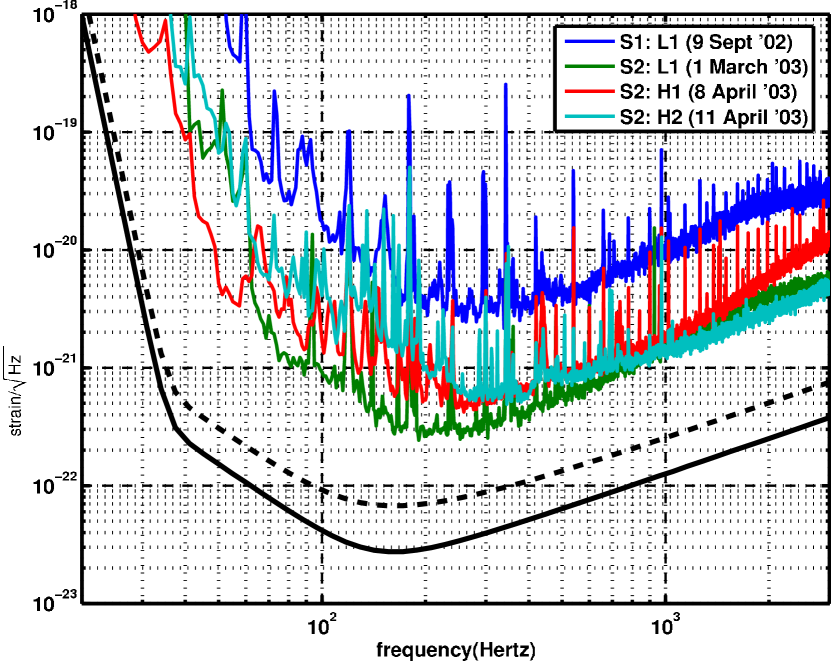
Figure 1: Typical sensitivities, expressed as amplitude spectral densities of detector noise converted to equivalent gravitational-wave strain, for the best detector during the S1 run (the Livingston detector) and for all three detectors during the S2 run. The solid lower line is the design sensitivity for the LIGO 4-km detectors; the dashed line is the design sensitivity for the LIGO 2-km detector at Hanford.

The amount of science data with good performance and stable operating conditions was limited by environmental factors (especially high ground motion at LLO and strong winds at LHO), occasional equipment failures, and periodic special investigations. Over the 1415 hour duration of the S2 run, the total amount of science data obtained was 536 hours for L1, 1044 hours for H1, and 822 hours for H2.

The analysis presented here uses data collected while the LLO detector was operating at the same time as one or both of the LHO detectors. Science data during which both H1 and H2 were operating but L1 was not, amounting to 385 hours, was not used in this analysis because of concerns about possible environmentally-induced correlations between the data streams of these two co-located detectors; this data set, as well as data collected while only one of the LIGO detectors was in science mode, will be used in a separate analysis together with data from the TAMA300 detector Ando et al. (2001), which conducted “Data Taking 8” concurrently with the LIGO S2 run.

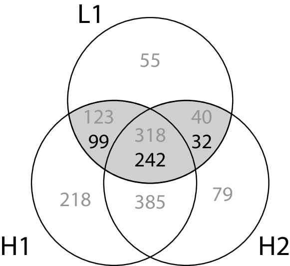
Figure 2: The number of hours that each detector combination was operational during the S2 run. The upper number gives the amount of time the specific instruments were coincidentally operational. The lower number gives the total time that was searched for inspiral triggers. The shaded region corresponds to the data used in this search.

Of all the data, approximately 9% (uniformly sampled within the run so as to be representative of the whole data set) was used as playground data for tuning parameters and thresholds in the analysis pipeline, and for use in identifying vetoes that were effective in eliminating spurious events. This playground data set was excluded from the gravitational wave inspiral upper limit calculation because event selection and pipeline tuning, as described in Secs. IV, V and VI, introduces statistical bias which cannot be accounted for. The playground data set was searched for inspiral signals, however, so a potential detection during these times was not excluded. After applying data quality cuts (as detailed in Sec. V) and accounting for short time intervals which could not be searched for inspiral signals by the filtering algorithm (described in Sec. IV), the observation time consisted of 242 hours of triple-detector data, plus 99 hours of L1-H1 and 32 hours of L1-H2 data, for a total observation time of 373 hours. For the upper limit result, the non-playground observation time was $339$ hours. A summary of the amount of single, double and triple detector times is provided in Fig. 2.

As with earlier analyses of LIGO data Abbott et al. (2004b), the output of the antisymmetric port of the detector was calibrated to obtain a measure of the relative strain $s=\Delta L/L$ of the detector arms, where $\Delta L=L_{x}-L_{y}$ is the difference in length between one arm (the $x$ arm) and the other (the $y$ arm), and $L$ is the average arm length. Reference calibration functions, tracing out the frequency-dependent response of the detectors, were measured (by moving the end mirrors of the detector with a known displacement) before and after the science run, and once during the science run; all three measurements gave consistent results. The changing optical gain of the calibration was monitored continuously during the run by applying sinusoidal motions with fixed frequency to the end mirrors. This continuous monitoring, averaged once a minute, allowed for small corrections to the calibration due to loss of light power in the arms, which can be caused by drifting optical alignment.

III Target Sources

Binary neutron star systems in the Milky Way, known from radio pulsar observations Stairs (2004), provide indirect evidence for the existence of gravitational waves Weisberg and Taylor (2003). Based on current astrophysical understanding, the spatial distribution of binary neutron stars is expected to follow that of star formation in the Universe. A measure of star formation is the blue luminosity of galaxies appropriately corrected for dust extinction and reddening. Therefore we model the spatial distribution of double neutron stars according to the corrected blue-light distribution of nearby galaxies Phinney (1991). While the masses of neutron stars in the few known binary systems are all near $1.4M_{\odot}$, population synthesis simulations suggest that some systems will have component masses as low as $\sim 1M_{\odot}$ and as high as the theoretical maximum neutron star mass of $\sim 3M_{\odot}$ Belczynski et al. (2002). Thus, we search for inspiral signals from binary systems with component masses in this range. Note that the higher-mass systems radiate more energy in gravitational waves and can thus be detected at a greater distance at a given SNR. For component masses below $1M_{\odot}$, a search is reported in Ref. Abbott et al. (2005b).

When the LIGO detectors reach their design sensitivities, they will be capable of detecting inspiral signals from thousands of galaxies, reaching beyond the Virgo Cluster for systems with optimal location and orientation. At that sensitivity, the rate of detectable binary neutron star coalescences could be as high as $0.7$ per year, though it is more likely to be an order of magnitude smaller Kalogera et al. (2004). For this analysis, our target population includes the Milky Way and all significant galaxies within a distance of 3 Mpc, which is roughly the maximum distance for which a $3$–$3M_{\odot}$ inspiral could be detected in coincidence by the L1 and H1 interferometers with a SNR of 6 in H1. This population includes the Local Group of galaxies, whose total blue-luminosity is dominated by the Andromeda Galaxy (M31), as well as some galaxies from neighboring groups. We cannot hope to detect all inspirals within this volume, because most systems in the population have lower masses and because the received signal amplitude is reduced, on average, depending on the orientation and location of the source relative to the detector.

Table 1 gives the parameters we use for the galaxies in the target population out to 1.5 Mpc, i.e., the maximum distance for which we had a non-zero detection efficiency in our simulations. The coordinates and distances of the galaxies in Table 1 are taken from a catalog by Mateo Mateo (1998), when available; this catalog is favored because distances quoted are from individual, focused studies of each of the nearby galaxies he includes. The rest of the distances, with only 100 kpc accuracy, are taken from the Tully Nearby Galaxies catalog Tully (1994). Data for blue luminosities are derived from the apparent blue magnitudes (corrected for reddening) quoted in Ref. de Vaucouleurs et al. (1991), and the distances shown in Table 1. We measured the efficiency of our search using Monte Carlo simulations, where the sources in the target population had a mass distribution as described in Ref. Belczynski et al. (2002), following the same guidelines as in the population models used in Ref. Nutzman et al. (2004). We used simulations with a population of neutron stars from galaxies up to 3 Mpc away, over-extending our target population, although we did not detect any simulated injections from sources farther than 1.5 Mpc away.

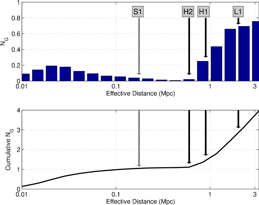
Figure 3: The upper panel shows the histogram of the number of Milky Way Equivalent Galaxies ($N_{G}$) as a function of effective distance. Labeled arrows indicate the average range of the best detector in the first science run (S1), as well as the average range of each detector during the second science run. The cumulative total within a given effective distance is shown in the bottom panel.

Table 1: The galaxies in our population within 1.5 Mpc. The next to last column indicates the number of injections detected in coincidence (with signal-to-noise-ratio defined in Eq. 10 satisfying $\rho^{2}>89$), over the number of injections performed in our simulations. The last column indicates the cumulative number of equivalent Milky Way galaxies contributed by systems within the corresponding distance, calculated from the search efficiency and the blue light luminosity.

	Right Ascension	Declination	Distance	Blue light luminosity	Detected/Injected	Cumulative
Name	(Hour:Min)	(Deg:Min)	(kpc)	relative to Milky Way	with $\rho^{2}>89$	$N_{G}$
Milky Way	—	—	—	1	686/686	1
LMC	+05:23.6	-69:45	49	0.128	57/57	1.128
SMC	+00:52.7	-72:50	58	0.037	8/8	1.165
NGC6822	+19:44.9	-14:49	490	0.01	0/4	1.165
NGC185	+00:39.0	+48:20	620	0.007	1/3	1.1673
M110	+00:40.3	+41:41	815	0.018	5/100	1.1682
M31	+00:42.7	+41:16	770	2.421	108/1791	1.3142
M32	+00:42.7	+40:52	805	0.019	9/129	1.3155
IC10	+00:20.4	+59:18	825	0.031	1/10	1.3186
M33	+01:33.9	+30:39	840	0.319	9/219	1.3318
NGC300	+00:54.9	-37:41	1200	0.052	1/40	1.3331
M81	+09:55.6	+69:04	1400	0.196	1/147	1.3344
NGC55	+00:14.9	-39:11	1480	0.175	2/122	1.3373

Within the LIGO frequency band, the gravitational waveform produced by binary neutron star systems is well described by the restricted second-post-Newtonian approximation Apostolatos (1995); Droz and Poisson (1997); Droz (1999). The spins of the neutron stars are not expected to significantly affect the orbital motion or the waveform Apostolatos (1995). Tidal coupling and other finite-body effects dependent on the equation of state also are not expected to significantly affect the waveform in the LIGO band Bildsten and Cutler (1992). The waveform received at Earth is therefore parameterized by the masses of the companions, the distance to the binary, the inclination of the system to the plane of the sky, and by the initial orbital phase when the waveform enters the LIGO band. The waveforms consist of two polarizations, the plus ($h_{+}$) and cross ($h_{\times}$) polarizations, which describe the two orthogonal tidal distortions produced by the waves. These polarization basis states are defined with respect to the orientation of the binary orbit relative to the line of sight. An interferometric detector is sensitive to a particular linear combination of these two polarizations; this is described by two response functions $F_{+}$ and $F_{\times}$ so that the expected gravitational-wave signal is

$$h(t)=F_{+}h_{+}(t)+F_{\times}h_{\times}(t).$$ (1)

The response functions depend on the location of the detector on the Earth and on the orientation of the detector’s arms. The interferometers at LHO and LLO are aligned as closely as possible, but the curvature of the Earth causes a slight difference in their antenna patterns.

IV Filtering and Trigger Generation

We generated event triggers by filtering the data $s(t)$ from each detector with matched filters designed to detect the expected signals. For any given binary neutron star mass pair, $\{m_{1},m_{2}\}$, we constructed the expected frequency-domain inspiral waveform template, $\tilde{h}(f)$, using a stationary phase approximation to the restricted second post Newtonian waveform Blanchet et al. (1996). Here, the tilde indicates the Fourier transform of a time series $h(t)$ according to the convention

$$\tilde{h}(f)=\int_{-\infty}^{\infty}h(t)e^{-2\pi ift}dt.$$ (2)

The matched filter output is then the complex time series

$$z(t)=x(t)+iy(t)=4\int_{0}^{\infty}\frac{\tilde{h}^{\ast}(f)\tilde{s}(f)}{S(f)}\,e^{2\pi ift}df$$ (3)

where $x(t)$ is the (real) matched filter output for the inspiral waveform with a zero orbital phase, and $y(t)$ is the (real) matched filter output for the inspiral waveform with a $\pi/2$ orbital phase. The quantity $S(f)$ is the one-sided strain noise power spectral density, estimated from the data. The matched filter variance is given by

$$\sigma^{2}=4\int_{0}^{\infty}\frac{|\tilde{h}(f)|^{2}}{S(f)}df$$ (4)

which depends on the template’s amplitude normalization. The amplitude signal-to-noise ratio (SNR) is then

$$\rho=|z|/\sigma\,.$$ (5)

The templates were normalized to a binary neutron star inspiral at an effective distance of 1 Mpc, where the effective distance of a waveform is the distance for which a binary neutron star system would produce the waveform if it were optimally oriented. Thus,

$$D_{\mathrm{eff}}=\frac{\sigma}{\rho}$$ (6)

is an estimate of the effective distance, in Mpc, of a putative signal that produces SNR $\rho$.

Since each binary neutron star mass pair $\{m_{1},m_{2}\}$ would produce a slightly different waveform, we constructed a bank of templates with different mass pairs such that, for any actual mass pair with $1\,M_{\odot}\leq m_{2}\leq m_{1}\leq 3\,M_{\odot}$, the loss of SNR due to the mismatch of the true waveform from that of the best fitting waveform in the bank is less than $3\%$ Owen (1996); Owen and Sathyaprakash (1999).

Although a threshold on the matched filter output $\rho$ would be the optimal detection criterion for an accurately-known inspiral waveform in the case of stationary, Gaussian noise, the character of the data used in this analysis is known to be neither stationary nor Gaussian. Indeed, many classes of transient instrumental artifacts have been categorized, some of which produce copious numbers of spurious, large SNR events. In order to reduce the number of spurious event triggers, we adopted a now-standard $\chi^{2}$ requirement Allen (2005): The matched filter template is divided into $p$ frequency bands, which are chosen so that each band would contribute a fraction $1/p$ of the total SNR if a true signal (and no detector noise) were present. In our analysis, we used $p=15$, as explained in Sec. VI.2. We then construct a chi-squared statistic comparing the magnitude and phase of SNR accumulated in each band to the expected amount. For a true signal in Gaussian noise, the resulting statistic is $\chi^{2}$ distributed with $2p-2$ degrees of freedom (since the SNR is constructed out of the two matched filters $x$ and $y$ which are both measured). Instrumental artifacts tend to produce very large $\chi^{2}$ values and can be rejected by requiring $\chi^{2}$ to be less than some reasonable threshold. Due to the discreteness of the template bank, however, a real signal will generally not match precisely the nearest template in the bank. Consequently, $\chi^{2}$ has a non-central chi-squared distribution with non-centrality parameter $\lambda\leq(p-1)\rho^{2}\mu^{2}$, where $\mu$ is the fractional loss of SNR due to mismatch between template and signal Allen (2005). For sufficiently small $\mu$ and moderate values of $\rho$, this effect is not important, but when $\rho$ is large, it must be taken into account. This is done by applying a threshold with the following parametrization:

$$\chi^{2}\leq{(p+\delta^{2}\rho^{2})}\xi^{\ast}\,.$$ (7)

The threshold multiplier $\xi^{\ast}$, the number of bins $p$ and the value of $\delta$ were determined by tuning on the playground data, as will be described in Sec. VI.2.

In this analysis, the SNR $\rho(t)$ was computed for each template in the bank. Whenever $\rho(t)$ exceeded a threshold $\rho^{\ast}$, the value of $\chi^{2}$ was computed for that time. If $\chi^{2}$ was below the threshold in Eq. (7), then the local maximum of $\rho(t)$ was recorded as a trigger. Each trigger is represented by a vector of values: the masses which define the template, the maximum value of $\rho$ and corresponding value of $\chi^{2}$, the inferred coalescence time, the effective distance $D_{\mathrm{eff}}$, and the coalescence phase $\phi_{0}=\tan^{-1}(y/x)$.

V Data Quality Checks and Vetoes

In practice, the performance of the matched filtering algorithm described above is influenced by non-stationary optical alignment, servo control settings, and environmental conditions. We used two strategies to avoid problematic data in this search. One was to evaluate data quality over relatively long time intervals, using several different tests. Time intervals identified as being suspect or demonstrably bad were skipped when filtering the data. The other method was to look for signatures in environmental monitoring channels and auxiliary interferometer channels which would indicate an external disturbance or instrumental glitch (a large transient fluctuation), allowing us to veto any triggers recorded at that time.

Several data quality tests were applied a priori, leading us to omit data when calibration information was missing or unreliable, servo control settings were not at their nominal values, or there were input/output controller timing problems. Additional tests were performed to characterize the noise level in the interferometer in various frequency bands and to check for problems with the photodiodes and associated electronics. The playground data set was used to judge the relevance of these additional tests, and two data quality tests were found to correlate with inspiral triggers found in the playground. One of these pertained only to the H1 interferometer; there were occasional, abnormally high noise levels in the H1 antisymmetric port channel that were apparent when this signal was averaged over a minute. Data was rejected only if this excessive noise was present for at least 3 consecutive minutes. The other data quality test used to reject data pertained to saturation of the photodiode at the antisymmetric port. These photodiode saturation events correlated with a small, but significant, number of L1 inspiral triggers. We required the absence of photodiode saturation in the data from all three detectors.

A gravitational wave would be most evident in the signal obtained at the antisymmetric port. We examined many other auxiliary interferometer channels, which monitor the light in the interferometer at points other than the antisymmetric port, to look for correlations between glitches found in the readouts of these channels and inspiral event triggers found in the playground data. These auxiliary channels are sensitive to certain instrumental artifacts which may also affect the antisymmetric port, and therefore may provide highly effective veto conditions. Although these channels are expected to have little or no sensitivity to a gravitational wave, we considered the possibility that an actual astrophysical signal could produce the observed glitches in the auxiliary channel due to some physical or electronic coupling. This possibility was tested by means of hardware injections, in which a simulated inspiral signal is injected into the data by physically moving one of the end mirrors of the interferometer. These hardware injections were used for validation of the analysis pipeline, as described in Sec. VI.3. Unlike the software injections that are used to measure the pipeline efficiency (described in Sec. VI.2), these hardware injections allow us to establish a limit on the effect that a true signal would have on the auxiliary channels. Only those channels that were unaffected by the hardware injections were considered safe for use as potential veto channels.

We used an analysis program, glitchMon, Ito to identify large amplitude transient signals in auxiliary channels. Numerous channels were examined by glitchMon, which generates a list of times when glitches occurred, identified by a filtered time series crossing a chosen threshold. A veto condition based on a given list of glitchMon triggers was defined by choosing a fixed time window around each glitch and rejecting any inspiral event trigger with a coalescence time within the window.

For each veto condition considered, we evaluated the veto efficiency (percentage of inspiral events eliminated), use percentage (percentage of veto triggers which veto at least one inspiral event), and dead-time (percentage of science-data time eliminated by the veto). Once a channel was identified, some tuning was done of the filters used, and the thresholds and time windows chosen, to optimize the efficiency, especially for high SNR candidates, without an excessive deadtime. The parameter tuning was done only with the inspiral triggers found in the playground.

No efficient candidate veto channels were identified for H1 and H2; there were some candidates for L1. Non-stationary noise in the low-frequency part of the sensitivity range used for the inspiral search appeared to be the dominant cause for glitch events in the data. The original frequency range for the binary neutron star inspiral search extended from $50$ Hz to $2048$ Hz. It was discovered that many of the L1 inspiral triggers appeared to be the result of non-stationary noise with frequency content around $70$ Hz. An important auxiliary channel, L1:LSC-POB_I, proportional to the length fluctuations of the power recycling cavity, was found to have highly variable noise at $70$ Hz. As a consequence, it was decided that the low-frequency cutoff of the binary neutron star inspiral search should be increased from 50 Hz to $100$ Hz. This subsequently reduced the number of inspiral triggers. An inspection of artificial signals injected into the data revealed a very small loss of efficiency for binary neutron star inspiral signal detection resulting from the increase in the low-frequency cutoff.

Even after raising the low-frequency cutoff, the L1:LSC-POB_I channel was found to be an effective veto when filtered appropriately. Due to the characteristics of the inspiral templates’ response to large glitches, we decided to veto with a very wide time window, $-4$ s to $+8$ s, around the time of each L1:LSC-POB_I trigger. With this choice, 12 % of the BNS inspiral triggers with $\rho>8$ in the playground were vetoed, as well as 5 out of the 9 triggers found in the playground with $\rho>10$. The use percentage of the veto triggers was 18 % for $\rho>8$ and 0.7 % for $\rho>10$, whereas values of 3 % and $<0.1$ % (respectively) would be expected from random coincidences if the veto triggers had no real correlation with the inspiral triggers. The total L1 dead-time using this veto condition in the playground was 2.7 %. The performance in the full data set was consistent with that found in the playground: the final observation time (including playground) was reduced by this veto from 385 hours to 373 hours. A more extensive discussion of LIGO’s S2 binary inspiral veto study can be found in Christensen et al. (2004a).

VI Search for Coincident Event Candidates

VI.1 Analysis Pipeline

The detection of a gravitational-wave inspiral signal in the S2 data would (at the least) require triggers in L1 and one or more of the Hanford instruments with consistent arrival times (separated by the light travel time between the detectors) and waveform parameters. Requiring temporal coincidence between the two observatories greatly reduces the background rate due to spurious triggers, thus allowing an increased confidence for detection candidates. When detectors at both observatories are operating simultaneously, we may obtain an estimate of the rate of background triggers by time-shifting the Hanford triggers with respect to the Livingston triggers and applying the same coincidence requirements to the time-shifted triggers, as described in Sec. VII. In this way, we can measure the rate of accidental coincidences in our search.

During the S2 run, the three LIGO detectors had substantially different sensitivities. The sensitivity of the L1 detector was greater than that of either Hanford detector throughout the run. Since the orientations of the LIGO interferometers are similar, we expect that signals of astrophysical origin detected in the Hanford interferometers generally are detectable in the L1 interferometer. Using this as a guiding principle, we have constructed a triggered search pipeline, summarized in Fig. 4. We search for inspiral triggers in the most sensitive interferometer (L1), and only when a trigger is found in this interferometer do we search for a coincident trigger in the less sensitive interferometers. This approach reduces significantly the computational power necessary to perform the search, without compromising the detection efficiency of the pipeline.

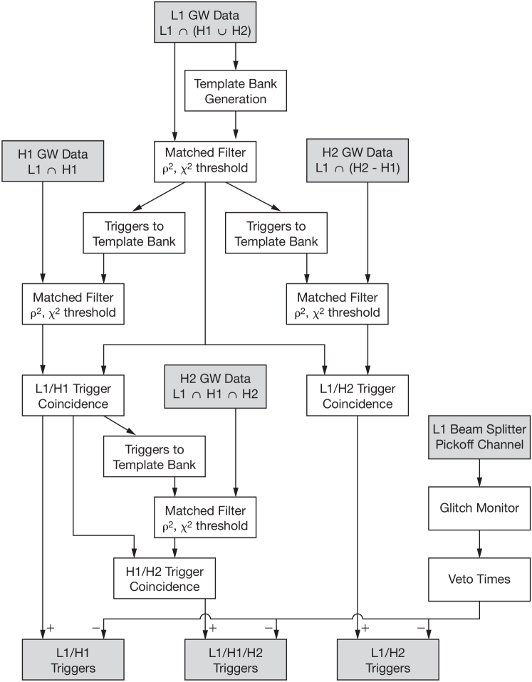
Figure 4: The inspiral analysis pipeline used to determine the reported upper limit. $\mathrm{L1}\cap(\mathrm{H1}\cup\mathrm{H2})$ indicates times when the L1 interferometer was operating in coincidence with one or both of the Hanford interferometers. $\mathrm{L1}\cap\mathrm{H1}$ indicates times when the L1 interferometer was operating in coincidence with the H1 interferometer. $\mathrm{L1}\cap(\mathrm{H2}-\mathrm{H1})$ indicates times when the L1 interferometer was operating in coincidence with only the H2 interferometer. The outputs of the search pipeline are triggers that belong to one of the two double-detector coincident data sets or to the triple-detector data set.

Times when each interferometer was in stable operation are called science segments. The science segments from each interferometer are used to construct three data sets corresponding to: (1) times when all three interferometers were operating, (2) times when only the L1 and H1 interferometers were operating; and (3) times when only the L1 and H2 interferometers were operating. The pipeline produces a list of coincident triggers for each of these three data sets as described below.

The science segments were analyzed in chunks of 2048 seconds using the findchirp implementation of matched filtering for inspiral signals in the LIGO Algorithm library LAL . In this code, the data set for each 2048 second chunk is first down-sampled from 16384 Hz to 4096 Hz. It is subsequently high-pass filtered and a low frequency cutoff of 100 Hz imposed. The calibrated instrumental response for the chunk is calculated using the average of the calibrations (measured every minute) over the duration of the chunk.

Triggers are not searched for within the first and last $64$ s of a given chunk, so subsequent chunks are overlapped by $128$ s to ensure that all of the data in a continuous science segment (except for the first and last 64 seconds) are searched for triggers. Any science segments shorter than $2048$ s are ignored. If a science segment cannot be exactly divided into overlapping chunks (as is usually the case) the remainder of the data set is covered by a special $2048$-s chunk which overlaps with the previous chunk as much as necessary to allow it to reach the end of the segment. For this final chunk, a parameter is set to restrict the inspiral search to the time interval not covered by any previous chunk, as shown in Fig 5.

Each chunk is further split into 15 analysis fragments of length 256 seconds overlapped by 128 seconds. The power spectrum $S(f)$ for the 2048 seconds of data is estimated by taking the median of the power spectra of the 15 segments. (We use the median and not the mean to avoid biased estimates due to large outliers, produced by non-stationary data.) The average calibration is applied to the data in each analysis fragment, and the matched filter output in Eq. (3) is computed for each template in the template bank.

In order to avoid end-effects when applying the matched filter, the frequency-weighting factor, nominally $1/S(f)$, is altered so that its inverse Fourier transform has a maximum duration of $\pm 16$ seconds. The output of the matched filter near the beginning and end of each segment is corrupted by end-effects due to the finite duration of the power spectrum weighting and also the inspiral template. By ignoring the filter output within 64 s of the beginning and end of each segment, we ensure that only uncorrupted filter output is searched for inspiral triggers. This necessitates the overlapping of segments and chunks as described above.

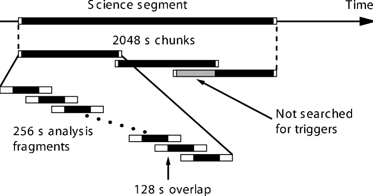
Figure 5: The algorithm used to divide science segments into data analysis fragments. Science segments are divided into $2048$ s chunks overlapped by $128$ s. (Science segments shorter than $2048$ s are ignored.) An additional chunk with a larger overlap is added to cover any remaining data at the end of a science segment. Each chunk is divided into $15$ analysis fragments of length $256$ s for filtering. The first and last $64$ s of each analysis fragment are ignored, so the segments overlap by $128$ s. Areas shaded black are searched for triggers by the search pipeline. The gray area in the last chunk of the science segment is not searched for triggers as this time is covered by the preceding chunk, although these data points are used is used in estimating the noise power spectral density for the final chunk.

The power spectral density (PSD) of the noise in the Livingston detector is estimated independently for each L1 chunk that is coincident with operation of a Hanford detector [denoted $\mathrm{L1}\cap(\mathrm{H1}\cup\mathrm{H2})$]. The PSD is used to lay out a template bank for filtering that chunk, according to the parameters for mass ranges and minimal match Owen (1996); Owen and Sathyaprakash (1999). The data from the L1 interferometer for the chunk are then filtered, using that bank, with a signal-to-noise threshold $\rho_{\mathrm{L}}^{\ast}$ and $\chi^{2}$ veto threshold $\xi^{\ast}_{\mathrm{L}}$ to produce a list of triggers as described in Sec. IV. For each chunk in the Hanford interferometers, a triggered bank is created consisting of every template which produced at least one trigger in L1 during the time of the Hanford chunk. This is used to filter the data from the Hanford interferometers with signal-to-noise and $\chi^{2}$ thresholds specific to the interferometer, giving a total of six thresholds that may be tuned. For times when only the H2 interferometer is operating in coincidence with L1 [denoted $\mathrm{L1}\cap(\mathrm{H2}-\mathrm{H1})$] the triggered bank is used to filter the H2 chunks that overlap with L1 data; these triggers are used to test for L1/H2 coincidence. All H1 data that overlaps with L1 data (denoted $\mathrm{L1}\cap\mathrm{H1}$) are filtered using the triggered bank for that chunk. For H1 triggers produced during times when all three interferometers were operating, a second triggered bank is produced for each H2 chunk consisting of every template which produced at least one trigger found in coincidence in L1 and H1 during the time of the H2 chunk. The H2 chunk is filtered with this bank. Any H2 triggers found with this bank are tested for triple coincidence with the L1 and H1 triggers. The remaining triggers from H1, when H2 is not available, are used to search for L1/H1 coincident triggers.

For a trigger to be considered coincident between two interferometers, the following conditions must be fulfilled: (1) Triggers must be observed in both interferometers within a temporal coincidence window that allows for the error in measurement of the time of the trigger, $\delta t$. If the detectors are not co-located, this parameter is increased by the light travel time between the observatories ($10$ ms for traveling 3000 km at the speed of light). (2) We then ensure that the triggers have consistent waveform parameters by demanding that the two mass parameters for the template are identical to within an error of $\delta m$. (3) For H1 and H2, we may impose an amplitude cut on the triggers given by

$$\frac{\left|D_{\mathrm{1}}-D_{\mathrm{2}}\right|}{D_{\mathrm{1}}}<\frac{\epsilon}{\rho_{\mathrm{2}}}+\kappa,$$ (8)

where $D_{1}$ ($D_{2}$) is the effective distance of the trigger in the first (second) detector and $\rho_{2}$ is the signal-to-noise ratio of the trigger in the second detector. The parameters $\epsilon$ and $\kappa$ are tunable. As shown in Fig. 6, the non-perfect alignment of LLO and LHO (due to their different latitudes) can occasionally cause large variations in the detected signal amplitudes for astrophysical signals. In order to disable the amplitude cut when comparing triggers from LLO and LHO, we set $\kappa=1000$.

If the detectors are at the same site, we ask if the maximum distance to which H2 can see at the signal-to-noise threshold $\rho_{\mathrm{H2}}^{\ast}$ is greater than the distance of the H1 trigger, allowing for errors in the measurement of the trigger distance. If this is the case, we demand time, mass and effective distance coincidence. If the distance to which H2 can see overlaps the error in measured distance of the H1 trigger, we search for a trigger in H2, but always keep the H1 trigger even if no coincident trigger is found. If the minimum of the error in measured distance of the H1 trigger is greater than the maximum distance to which H2 can detect a trigger we keep the H1 trigger without searching for coincidence.

If coincident triggers are found in H1 and H2, we can get an improved estimate of the amplitude of the signal arriving at the Hanford site by coherently combining the filter outputs from the two gravitational wave channels,

$$\rho_{H}=\sqrt{\frac{|z_{H1}+z_{H2}|^{2}}{\sigma_{H1}^{2}+\sigma_{H2}^{2}}}\;.$$ (9)

The more sensitive interferometer receives more weight in this combination, as can be seen from Eq. (3), in which the noise enters in the denominator. If a trigger is found in only one of the Hanford interferometers, then $\rho_{H}$ is simply taken to be the value of $\rho$ from that interferometer.

The final step of the search is to apply the POB_I veto, described in Sec. V, to eliminate certain L1 triggers which arose from instrumental glitches. The individual signal-to-noise ratios are used to construct a multi-detector statistic as described in Sec. VIII for any surviving triggers.

The surviving coincident triggers are clustered in a way that identifies the best parameters to associate with a possible inspiral signal in the data. The clustering is needed since large astrophysical signals and instrumental noise bursts can produce many triggers with coalescence times within a few seconds of each other. We chose the trigger with the largest SNR from each cluster; triggers separated by more than 4 seconds were considered unique. Alternative clustering methods are discussed in Sec. VII in an effort to understand the accidental likelihood of a small number of candidates that were observed in the final sample.

To perform the search on the full data set, a directed acyclic graph (DAG) was constructed to describe the work flow, and execution of the pipeline tasks was managed by Condor Tannenbaum et al. (2001) on the UWM and LIGO Beowulf clusters. The software to perform all steps of the analysis and construct the DAG is available in the package lalappsLAL .

VI.2 Parameter Tuning

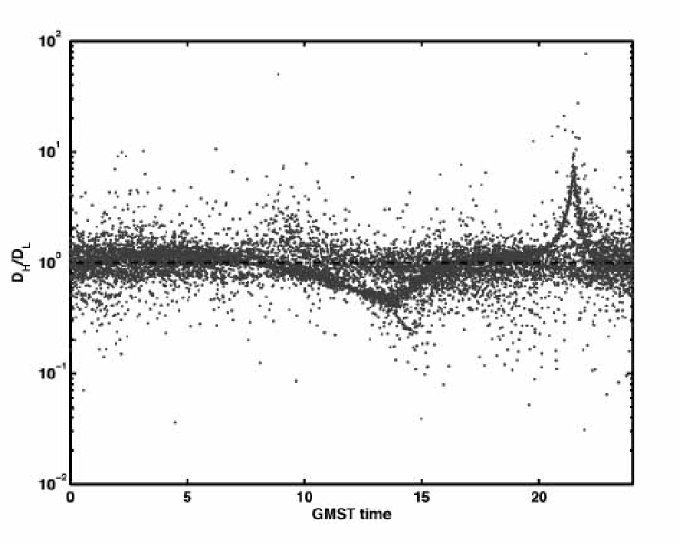
Figure 6: Ratio of effective distance at the Hanford and Livingston Observatories for the injections from sources in Table. 1, versus Greenwich mean Sidereal Time (GMST). The sharp feature near 21.5 hrs is due to M31 (Andromeda) passing through a sky position at the Hanford node, producing much larger effective distances at LHO than at LLO. The softer feature near 14 hrs is due to M33 (Triangulum Galaxy) passing through a similar sensitivity node for LLO. About 15% of injected signals have a $50\%$ difference or larger in the effective distance between the sites due to the slight mis-alignment of the detectors.

The entire analysis pipeline was studied first using the playground data set to tune the values of the various parameters. The goal of tuning was to maximize the efficiency of the pipeline to detection of gravitational waves from binary inspirals without producing an excessive rate of spurious candidate events. The detection efficiency was determined by Monte Carlo simulations in which we injected simulated inspiral signals from our model population into the data. The efficiency is the ratio of the number of signals detected to the number injected, as described in Sec. VI.2.1. In the absence of a detection, a pipeline with a high efficiency and low false alarm rate allows us to set a better upper limit, but it should be noted that our primary motivation is to enable reliable detection of gravitational waves. By evaluating the efficiency using Monte Carlo injection of signals from the hypothetical population of binary neutron stars into the data, we account for systematic effects caused by our vetoes and other aspect of our pipeline.

There are two sets of parameters that we can tune in the pipeline: (1) the single interferometer parameters which are used in the matched filter and $\chi^{2}$ veto to generate inspiral triggers in each interferometer, and (2) the coincidence parameters used to determine if triggers from two interferometers are coincident. The single interferometer parameters include the signal-to-noise threshold $\rho^{\ast}$, the number of frequency sub-bands $p$ in the $\chi^{2}$ statistic, the coefficient $\delta$ on the SNR dependence of the $\chi^{2}$ cut, and the $\chi^{2}$ cut threshold $\xi^{\ast}$. These are tuned on a per-interferometer basis, although some of the values chosen are common to two or three detectors. The coincidence parameters are the time coincidence window for triggers, $\delta t$, the mass parameter coincidence window, $\delta m$, and the effective distance cut parameters $\epsilon$ and $\kappa$ described in Eq. (8). Due to the nature of the triggered search pipeline, parameter tuning was carried out in two stages. We first tuned the single interferometer parameters for the primary detector (L1). We then used the triggered template banks (generated from the L1 triggers) to explore the single interferometer parameters for the less sensitive Hanford detectors. Finally, the parameters of the coincidence test were tuned.

VI.2.1 Single Interferometer Tuning

The number of bins $p$ used in the $\chi^{2}$ test was set to $p=15$ (compared with $p=8$ used in our S1 search Abbott et al. (2004b)), in order to better differentiate spurious triggers from actual (or injected) signals, while still having at least several cycles of the waveform in each bin.

The $\delta$ parameter in Eq. (7) is expected to be no less than 0.03 for our choice of maximum 3% SNR loss in the L1 template bank. A dedicated investigation using software injections into L1 showed that the $\chi^{2}$ test rejected 50% of signals from the Milky Way (with effective distances closer than 200 kpc) when using $\delta=0.03$; using $\delta=0.1$ recovered all such injections. The search efficiency for weaker injections, at effective distances larger than 900 kpc, did not depend on $\delta$.

The signal to noise threshold $\rho^{\ast}=6$ was used in all three instruments. This choice was motivated by the observation that a signal, with certain orbital orientations and sky positions, can have a smaller effective distance in the less sensitive detector (see next Sec VI.2.2 and Fig. 6). This choice of threshold was computationally possible due to our efficient pipeline and code; it also provided better statistics for background estimation (Sec VII).

Once the L1 search parameters had been tuned, the resulting triggered template banks were used as input to tune the H1 and H2 $\chi^{2}$ threshold parameters $\xi^{\ast}$ in the coincidence search. The final value was selected so that the triggered search suffered no loss of efficiency due to this single parameter. Table 2 shows how the parameter $\xi^{\ast}$ was tuned, first for L1 and then for H1. The values chosen for all parameters are shown in Table 3.

Table 2: The effect of lowering the $\chi^{2}$ threshold, $\xi^{\ast}$, for the single interferometer L1, and for the combination of L1 and H1 in the pipeline. The efficiency of the L1 search remains constant as the threshold is lowered to $5.0$, however as the threshold is lowered in H1, the efficiency of the triggered search drops. Further testing indicated that a threshold of $12.5$ in H1 was acceptable without a loss of efficiency.

Value of $\chi^{2}$ threshold, $\xi^{\ast}_{L1}$	L1 Efficiency	Pipeline Efficiency
20.0	0.350	0.270
15.0	0.350	0.270
10.0	0.350	0.255
5.0	0.350	0.212

VI.2.2 Coincidence Parameter Tuning

After the single interferometer parameters had been selected, the coincidence parameters were tuned. As described in Sec. VI.3, the coalescence time of an inspiral signal can be measured to within $\leq 1$ ms. The gravitational waves’ travel time between observatories is $10$ ms, so $\delta t$ was chosen to be $1$ ms for LHO-LHO coincidence and $11$ ms for LHO-LLO coincidence. The mass coincidence parameter was initially chosen to be $\delta m=0.03$, however testing showed that this could be set to $\delta m=0.0$ (i.e. requiring the triggers in each interferometer to be found with the exact same template) without loss of efficiency.

After tuning the time and mass parameters, we tuned the effective distance parameters $\kappa$ and $\epsilon$. Initial estimates of $\epsilon=2$ and $\kappa=0.2$ were used for testing, however we noticed that many injections were missed when testing for LLO-LHO distance consistency. This is due to the slight detector misalignment between the two sites from Earth’s curvature, which causes the ratio of effective distances, as measured at the two observatories, to be large for a significant fraction of our target population, as shown in Fig. 6. Consequently, we disabled the effective distance consistency requirement for triggers generated at different observatories. A study of simulated events injected into H1 and H2 suggested values of $\epsilon_{HH}=2$ and $\kappa_{HH}=0.5$ to be suitable. Note that, as described above, we demand that an L1/H1 trigger pass the H1/H2 coincidence test if the effective distance of the trigger in H1 is within the maximum range of the H2 detector at threshold.

Table 3: A complete list of the parameters that were selected at the various stages of the pipeline. The procedures used to select these parameter values are outlined in the text.

Parameter	Pipeline node	value
$\rho^{\ast}$	GW Data (all)	6.0
$p$	GW Data (all)	15
$\delta$	GW Data (all)	0.1
$\xi^{\ast}_{L}$	L1 GW Data	5.0
$\xi^{\ast}_{H}$	H1/H2 GW Data	12.5
$\delta t_{HH}$	H1/H2 Trigger Coincidence	0.001 s
$\delta t_{HL}$	L1/H1 and L1/H2 Trigger Coincidence	0.011 s
$\delta m$	Trigger Coincidence (all)	0.0
$\kappa_{HH}$	H1/H2 Trigger Coincidence	0.5
$\epsilon_{HH}$	H1/H2 Trigger Coincidence	2
$\kappa_{HL}$	L1/H1 and L1/H2 Trigger Coincidence	1000

VI.3 Validation

Hardware signal injections were used as a test of our data analysis pipeline. These injections allow us to study issues of instrumental timing and calibration, as well as to verify that the injected signals were indeed identified as triggers in our analysis pipeline. At intervals throughout S2, a predetermined set of inspiral and burst signals were injected into the instruments using the mirror actuators.

We examined six sets of hardware injections spread throughout the S2 science run. Each set had six $1.4\textrm{-}1.4M_{\odot}$ inspiral signals at effective distances spaced logarithmically between 500 kpc and 15 kpc, and four $1.0\textrm{-}1.0M_{\odot}$ inspirals at distances from 500 kpc to 62 kpc. Each strain waveform was calculated using the second order post-Newtonian expansion for an optimally oriented inspiral, and appropriately scaled for an inspiral at the desired effective distance. The strain was then converted into an injection signal into the $y$-arm of the interferometer, with the appropriate calibration to produce the desired differential strain.

Of these injections, five sets were injected simultaneously into all three instruments and the sixth was injected into L1 and H1 only. After the coincidence stage of the pipeline, 59 of the 60 injections produced a trigger in the appropriate template ($1.4$–$1.4M_{\odot}$ or $1.0$–$1.0M_{\odot}$). (The single missed injection had a $\chi^{2}$ value in L1 which was slightly above threshold.) This is an excellent test of every stage of our pipeline. L1 successfully produced triggers corresponding to the injections, which were then used to make triggered banks against which the Hanford instruments were analyzed. Both H1 and H2 produced triggers which were coincident with those in L1. Furthermore, the amplitude cut between H1 and H2 was effective. For the louder injections, the effective distance was consistent between the two instruments. In the case of more distant injections which did not produce triggers in H2, the coincidence stage of the pipeline allowed the L1–H1 coincident triggers to be kept even though no event was found in H2.

The pipeline was also run on an additional set of hardware injections at distances between 5 Mpc and 150 kpc. Of these injections, the most distant which produced coincident triggers were at 1.25 Mpc for the $1.4-1.4M_{\odot}$ injection and 620 kpc for the $1.0-1.0M_{\odot}$ injection. This is consistent with the sensitivity of H1 during the injection time, and with the efficiency measured in our software injections (Table 1).

The trigger times associated with the hardware injections all agreed with expectations to within 1 msec.

Hardware injections provide a powerful test of instrumental calibration. Any errors in the calibration of the instrument affect the measured effective distance to the inspiral. Uncertainties in distance measurements will contribute to errors in our detection efficiency. Additionally, they become important when requiring consistency of effective distance in triggers from the two Hanford instruments. To test the accuracy of the effective distance measurements, we used the loudest injections — namely the $1.4-1.4M_{\odot}$ injections with distances less than 100 kpc — so that systematic errors in distance measurement would dominate over noise. The effective distance of all such injections was accurate to within $20\%$. We found that for L1, the distance to injections was systematically underestimated by $5\%$, with a $4\%$ standard deviation. For H1, there was a systematic underestimation of $2\%$ with a standard deviation of $3\%$. For H2, we had a $2\%$ overestimation and a standard deviation of $5\%$. These errors are consistent with uncertainties in the calibration described in Sec. IX.1. Further details of the S2 hardware injections are available in Fairhurst et al. (2004).

A Markov chain Monte Carlo routine (MCMC) Christensen et al. (2004b) was also used to examine the injected signals. This provides a method of estimating the parameters of an injected signal. As an example, for a $1.4-1.4M_{\odot}$ injection at 125 kpc, the MCMC routine generated masses of $1.4003M_{\odot}$ and $1.3991~{}M_{\odot}$. The width of the 95 % confidence interval for each mass was $0.012~{}M_{\odot}$.

VII Background estimation

An event candidate which survives all cuts in our analysis pipeline, including coincidence, can arise either from a real gravitational-wave signal or from noise bursts which contaminate our data streams. We refer to the latter class of event candidates as background. These background events are caused by many different environmental and instrumental processes. Under the assumption that such processes are uncorrelated between the detectors at Hanford and Livingston, we estimated the rate for background events due to accidental coincidences by applying artificial time shifts $\Delta t$ to the triggers coming from the Livingston detector. These time-shift triggers were then fed into subsequent steps of the pipeline. For a given time-shift, the triggers that survived to the end of the pipeline represent a single trial output from our search (if no coincident gravitational-wave signals were present).

A total of 40 time-shifts were analyzed to estimate the background: $\Delta t=\pm 5$, $\pm 10$, $\pm 15$, $\pm 27$, $\pm 37$, $\pm 47$, $\pm 57$, $\pm 67$, $\pm 77$, $\pm 87$, $\pm 97$, $\pm 107$, $\pm 117$, $\pm 127$, $\pm 137$, $\pm 147$, $\pm 157$, $\pm 167$, $\pm 177$, $\pm 197$ seconds. To avoid correlations, we used time-shifts longer than the duration of the longest template waveform ($\sim 4\textrm{ seconds}$). We did not time-shift the triggers from the Hanford detectors relative to one another since real correlations may arise from environmental disturbances. The resulting distribution of time-shift triggers in the $(\rho_{\mathrm{H}},\rho_{\mathrm{L}})$ plane was used to determine a joint signal to noise $\rho$. Here $\rho_{L}$ is given by Eq. (5) and $\rho_{H}$ is given by Eq. (9). For Gaussian noise fluctuations, with the single interferometer triggers’ SNR maximized over the polarization phase and the orbital inclination angle, one expects circular false alarm contours centered on the origin Pai et al. (2001), suggesting that the sum of the squares of the signal to noise ratios would be a useful combined statistic. The time-shifts revealed the need for a modified statistic; we settled on contours of (roughly) constant false-alarm probability to use in assigning a signal-to-noise to coincident triggers. As shown in Fig. 7, the combined SNR

$$\rho=\sqrt{\rho^{2}_{\mathrm{L}}+\rho_{\mathrm{H}}^{2}/4}$$ (10)

yielded approximate constant-density contours for the distribution of background events in the plane.

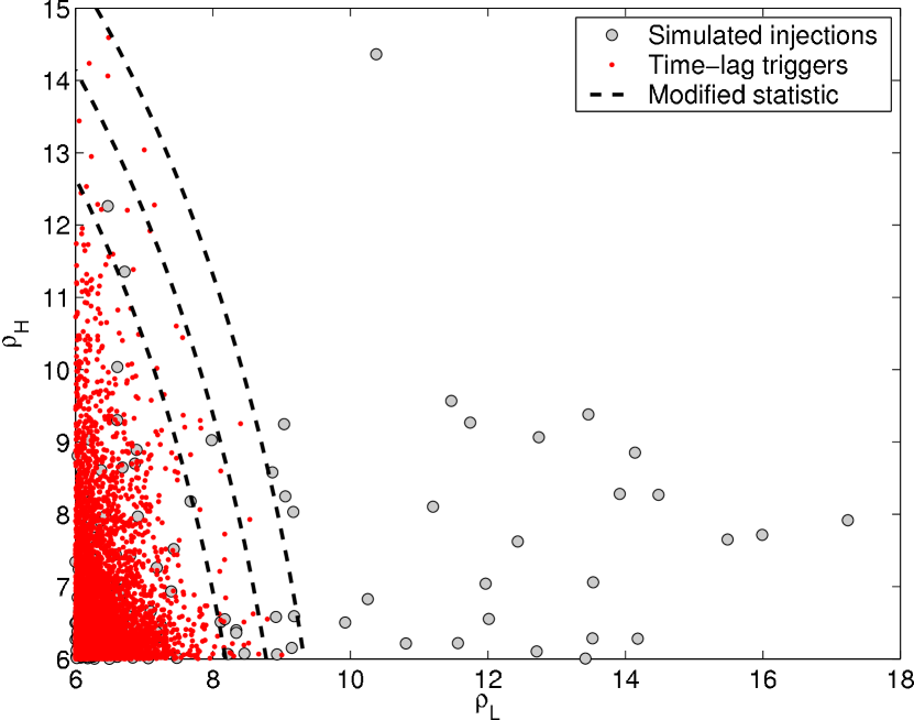
Figure 7: The signal to noise at Livingston $\rho_{\mathrm{L}}$ plotted against the signal to noise at Hanford $\rho_{\mathrm{H}}$ for triggers from 40 time-shifts. In Gaussian noise, one expects circular false alarm contours centered on the origin indicating that the sum of the squares of the signal to noise ratios would be a useful combined statistic. The observed distribution of time-shifted triggers motivated the modified statistic presented in Eq. (10).

Using data from the time-shifts, we also computed the (sample) mean number of events per S2 with $\rho>\rho^{*}$. This result is shown in Fig. 8; the shaded bars represent the sample variance for ease of comparison with the zero-shift distribution. The apparent exponential dependence of $b(\rho^{*})$ on $\rho^{*2}$ further supports the choice of combined statistic in Eq. (10).

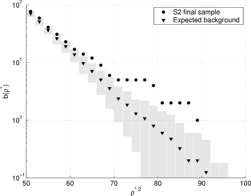
Figure 8: The number of triggers per S2 above combined SNR $\rho^{*}$. The triangles represent the expected (mean) background based on 40 time-shift analyses. The shaded envelope indicates the sample variance in the number of events. The choice of combined SNR in Eq. (10) is further justified by the behavior $b(\rho^{*})\propto exp(-\rho^{*2})$ down to about $0.3$ events per S2. The circles represent the un-shifted inspiral event candidates (Sec. VIII.1).

VIII Search Results

The pipeline described above was used to analyze the S2 data. The output of the pipeline is a list of candidate coincident triggers. To decide whether there is any plausible detection candidate worth following up, we compare the combined SNR of the candidates with the expected SNR from the accidental background. If the probability of any candidate being accidental is small enough, we look at the robustness of the parameters of the candidate under changes in the pipeline, and we investigate possible instrumental reasons for these candidates that may have been overlooked in the initial analysis.

Independently of whether detection candidates are found, we can use the results to set an upper limit on the rate of binary neutron star coalescences per Milky Way Equivalent Galaxy, per year. We use the same statistics as in the previous search in S1 data Abbott et al. (2004b), measuring the efficiency of the search at the SNR of the loudest trigger found. We take here the most conservative approach, taking into account all triggers at the output of the pipeline: both those triggers considered to be potential detection candidates and those that are consistent with being due to instrumental noise or consistent with background. We do not include the playground in the observation time used for calculating the upper limit, since the playground was used to the tune the pipeline. This is consistent with our approach of focusing on detection, and not optimizing the pipeline for upper limit results (which was the reason for not considering single detector data, for example).

As described in Section II, after the data quality cuts, discarding science segments with durations shorter than 2048 sec, and application of the instrumental veto in L1, a total of 373 hours of data were searched for signals, broken up in double and triple coincidence time as shown in Figure 2. For the upper limit analysis, including the background estimation, we only considered the non-playground times, amounting to 339 hours, of which 65% (221 hours) had all three detectors in operation; 26% (89 hrs) had only L1 and H1 in operation; and 8.5% (29 hrs) had only L1 and H2 in operation.

VIII.1 Triggers and event candidates

The output of the pipeline is a list of candidates which are assigned an SNR according to Eq. (10). There are 142 candidates in the non-playground final sample with combined $\rho^{2}$ greater than 45; the breakdown is 90 candidates from L1-H2 two detector data, 35 from triple detector data, and 17 from L1-H1 two detector data. All the candidates in the triple detector data had SNR in H1 too small to cross the threshold in H2, and following our pipeline, were accepted as coincident triggers. Thus, all our coincident triggers are only double-coincidence candidates.

Table 4 lists the ten largest SNR coincident triggers recorded in the analysis (including the playground). Detailed investigations of the conspicuous triggers were performed and are reported below. Nine out of these ten candidates were in the double detector sample. There was only one (#10 in the list) which was in the triple detector data, although it was too weak to require a corresponding trigger in H2. Our loudest candidate, as well as five of our loudest ten, are L1-H2 coincident triggers; in fact, 63% of all our candidates are L1-H2 coincident triggers. Since the L1-H2 data supplies only 9% of the total observation time, we conclude that the noise in H2 was significantly different than the noise in H1, producing more and louder triggers. For all triggers in Table 4, the effective distance is larger in the Livingston detector than in the Hanford detector: although this is plausible for real signals, as shown in Fig. 6, it suggests that these candidates are more likely to originate from instrumental noise.

Table 4: The 10 triggers with the largest SNR which remain at the end of the pipeline. This table indicates their UTC date, the time delay between Hanford and Livingston ($\delta t=t_{H}-t_{L}$), the combined SNR $\rho^{2}$ (from Eq. 10), the SNR registered in each detector, the value of $\chi^{2}$ per degree of freedom at each interferometer (for $2p-2=28$ d.o.f.), the effective distance to an astrophysical event with the same parameters in each detector, and the binary component masses of the best matching template (identical for the triggers in both detectors). The notation L1-Hx means that all three interferometers were in science mode at the time of this coincident trigger.

Rank	YYMMDD	$\delta t$	Instruments	$\rho^{2}$	$\rho_{L}$	$\rho_{H}$	$\chi^{2}/\text{d.o.f.}$	$\chi^{2}/\text{d.o.f.}$	$D^{L}_{\mathrm{eff}}$	$D^{H}_{\mathrm{eff}}$	$m_{1}$	$m_{2}$
	(UTC)	(ms)					(LLO)	(LHO)	(Mpc)	(Mpc)	($M_{\odot}$)	($M_{\odot}$)
# 1	030328	+9.8	L1-H2	89.1	8.9	6.1	2.6	3.4	2.1	0.9	2.23	2.23
# 2	030327	-1.7	L1-H2	87.1	7.6	11.0	2.7	5.1	2.1	0.7	2.09	2.09
# 3	030224	-7.6	L1-H2	79.5	6.5	12.3	1.2	6.4	2.6	0.4	3.04	1.19
# 4	030301	+7.1	L1-H1	79.0	7.7	8.8	2.3	4.7	2.1	0.6	1.45	1.45
# 5	030224	+5.4	L1-H1	77.2	6.7	11.3	1.9	6.5	2.0	0.5	1.90	1.35
# 6	030301	+11.0	L1-H1	69.2	6.7	9.9	2.0	5.9	2.2	0.5	1.28	1.28
# 7	030224	-1.5	L1-H2	67.2	6.9	8.9	1.3	4.1	2.7	0.8	2.46	1.82
# 8	030328	+4.4	L1-H2	67.1	7.4	7.2	2.8	2.3	1.9	0.6	2.27	1.11
# 9	030224	-10.5	L1-H1	66.5	6.9	8.8	1.6	4.3	2.3	0.8	3.60	1.20
# 10	030301	-1.7	L1-Hx	65.9	7.5	6.1	2.5	2.7	2.5	1.6	2.65	2.65

A trigger gets elevated to the status of an event candidate if the chance occurrence due to noise is small as determined by time-shift background estimation, calculated as described in Sec. VII. Each event candidate is subjected to follow-up investigations beyond the level of automation used in our pipeline to ensure that it is not due to an instrumental or environmental disturbance.

In Figure 8, a cumulative histogram of the final coincident triggers versus $\rho^{2}$ is overlayed on the expected background due to accidental coincidences, as determined by time-shifts. Even after taking into account that these are cumulative histograms, so that adjacent bins are strongly correlated, it appears that the number of coincident triggers is inconsistent with the expected background for large $\rho^{2}$. While the origin of this discrepancy is not understood, careful examination of the three coincident triggers with the highest $\rho^{2}$, detailed below, indicates that these are not gravitational wave detections. Moreover, no evidence of correlated noise between the Livingston and Hanford observatories was found for times around these triggers. In Sec. VIII.2, we demonstrate that a reasonable modification of our algorithm for clustering multiple coincident triggers results in good agreement between the coincident trigger sample and the background estimate. This shows that the background estimate is not robust with respect to reasonable variations in the analysis procedure.

In Sec. IX we derive an upper limit on the rate of inspiral events which is conservative with respect to any uncertainties in the background estimate. Thus, although the discrepancy between the coincident triggers and the background estimate presented in Fig. 8 is not understood, it does not affect our ability to detect inspiral signals or set an upper limit on the inspiral rate.

VIII.1.1 Trigger 030328

The loudest candidate is in a cluster of three coincident triggers in L1 and H2 on March 28, 2003. The loudest trigger in the cluster, # 1 in Table 4, has a large SNR in L1 ($\rho=8.9$), but an SNR in H2 ($\rho=6.1$) which is close to threshold for trigger generation. We expect a candidate arising from a real signal to be robust under small changes in our analysis pipeline. In order to test the robustness of this particular candidate upon changes in the boundaries for the chunks used in the analysis, we re-analyzed the data in this science segment shifting the start time of the chunk by different amounts in L1 and H2. Although in all cases our analysis produced similar numbers of triggers in each detector, only in the original case were there triggers within 11 ms that had identical masses and were considered candidates.

Other measured parameters of this trigger re-inforce the conclusion that it should not be promoted to a detection candidate. The $\chi^{2}$ per degree of freedom is bad, especially in H2 (3.4); the $\chi^{2}$ in L1 is close to our threshold [$\chi^{2}/(p+\delta^{2}\rho^{2})=4.6$ compared to the threshold $\xi^{\ast}=5$]. The effective distances measured by the detectors are very different, 2.1 Mpc in L1 and 0.9 Mpc in H2. This ratio of effective distances and the large time delay (10 ms) is unlikely, though not impossible, for the posited population. The other triggers in the cluster (with smaller SNR by definition) have a larger distance ratio, smaller time delay, smaller $\chi^{2}$, and different masses in the binary system (but the same masses in both triggers): $2.9M_{\odot}$ and $1.1M_{\odot}$.

The time series in the H2 detector does not show anything unusual in the gravitational wave channel or in other auxiliary channels: this is consistent with the small SNR measured in H2 for this trigger. The time series in L1, however, shows several disturbances in a few second window around the candidate. Many inspiral triggers are generated at the time although only three are coincident in mass and time with H2 triggers. Just 100 ms before the coalescence time of the trigger in question (and within the duration of the template corresponding to the trigger), we observed a fast fluctuation in the calibration, less than 62 ms in duration, indicating low optical gain dropping to levels that would make the feedback loop unstable. In the 51 minutes when the L1 detector was operational around the time of the candidate, such a low loop gain happened at three different instances. Each occurrence lasted less than 62 ms and was accompanied by a cluster of inspiral triggers generated by the search code. Since we averaged the calibration on a 60-second time scale, these rare fluctuations had not been observed when considering data quality. Nevertheless, such a low gain, even though brief, makes the data and its calibration very unreliable. This provides an instrumental reason to veto this trigger as a detection candidate: the cluster of triggers in L1 containing the coincident trigger was probably produced by non-linear effects associated with either the low gain itself or the alignment fluctuation that produced the low gain in the first place. An indication of this is that most of the excess power at the time of the trigger cluster is at sidebands of a narrow line in the spectrum, corresponding to up-conversion of low-frequency noise to the 120 Hz electric power line harmonic by some unknown bilinear process.

VIII.1.2 Trigger 030327

The second loudest candidate in Table 4 is on March 27, 2003; it is also an L1-H2 trigger, with a combined SNR $\rho^{2}=87$. Similar to the loudest candidate, according to the background estimates, it has a 20% false alarm probability. Unlike the loudest candidate, however, this trigger has a smaller SNR in L1 (7.6) than in H2 (11.0).

As shown in Fig. 9, there are four bursts of noise in the gravitational wave channel of the H2 detector in the 58 minutes surrounding this candidate when L1 and H2 were operating in coincidence. Each burst is a few to ten seconds long, and each triggers a large fraction of the template bank. Trigger 030327 is the loudest trigger in a cluster of seven L1-H2 coincident triggers, in a 3 ms interval, during one of the H2 noise bursts. There are also three other coincident triggers in the same noise burst, and there are clusters of coincident triggers in two of the other three H2 noise bursts. One of these bursts, with several coincident triggers, contains another one of our top twenty loudest candidates. The only noise burst that does not have any coincident triggers happens at a time when the H1 detector had begun operating, and the triple-coincidence criteria were not satisfied. In almost all of the time-shifts used to estimate the background, there were a number of L1-H2 coincident triggers at the time of the noise bursts in H2. We have not found the precise instrumental origin of the disturbances causing such large numbers of inspiral triggers: although simultaneous disturbances are observed in a few other auxiliary channels, none of them are as obvious as they are in the gravitational wave channel.

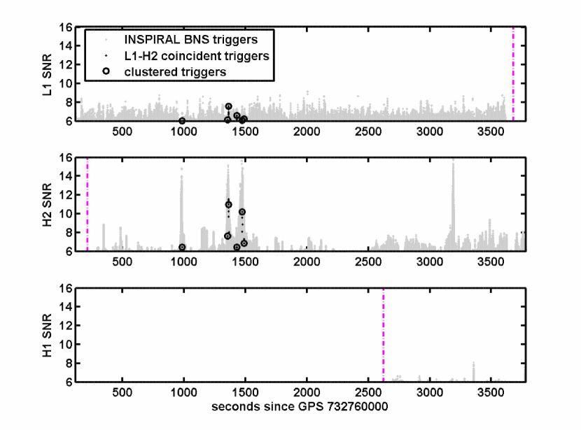
Figure 9: Triggers produced by the inspiral search in L1 (top panel), and the triggered search in H2 (middle panel) and H1 (lower panel), near the time of our second loudest candidate, on 03/03/27 UTC, in Table 4. The black points indicate the triggers that have identical mass and are coincident within a 11 ms window. The circles indicate the clustered candidate triggers. The dashed lines are the boundaries of the science segments in each detector (i.e, H1 and H2 were not operating to the left of the dashed line in their respective graphs, and L1 was not operating after the dashed line in the top panel) .

Despite a relatively low measured probability of this trigger being due to the background, we do not consider this trigger an event candidate due to the low SNR in the L1 detector, the poor $\chi^{2}$, the unlikely parameters, and a strong suspicion of instrumental misbehavior.

VIII.1.3 Trigger 030224

We also followed up the third loudest candidate on Feb 24, 2003. This is again an L1-H2 candidate, happening a few minutes before H2 turns off due to loss of the operating point at optical resonance. We discovered a very large feedback loop oscillation in an auxiliary servo operating in the orthogonal channel to the gravitational channel (L1:LSC-AS_I). Although the oscillation was at lower frequencies than the ones relevant for our search, it produced broadband excess power at all frequencies in two short time intervals, at the beginning and at the end of the oscillation. This instrumental misbehavior rules out this trigger as an event candidate.

VIII.2 Background estimation revisited

One striking feature of our analysis is the apparent discrepancy between the coincident trigger count in the zero-shift data set compared to our background estimate shown in Fig. 8. Our follow-up investigations rule out gravitational-wave signals as the origin of this discrepancy. Moreover, no evidence of correlated noise between the Livingston and Hanford observatories was found for times around these triggers. In an effort to understand how selection effects in our pipeline might be responsible for this apparent discrepancy, we repeated our analysis with a different method of clustering the coincident triggers at the end of our pipeline. Instead of selecting the trigger with the largest SNR from each cluster, we selected the coincident trigger with the minimum value of

$$\frac{\chi^{2}_{\mathrm{H}}}{p+\delta^{2}\rho_{\mathrm{H}}^{2}}+\frac{\chi^{2}_{\mathrm{L}}}{p+\delta^{2}\rho_{\mathrm{L}}^{2}}\;.$$ (11)

(Compare to Eq. 7.) We call this best-fit clustering since it preferentially selects events with small $\chi^{2}$ and/or large SNR. (See Sec. VI.1 for a description of the maximum SNR clustering.) The resulting background estimate and zero-shift distribution are shown in Fig. 10; no evidence of the original discrepancy remains.

Figure 11 compares the SNR under each clustering scheme for the final S2 trigger sample and a simulated injection run. The plot shows that the SNR from best-fit clustering is either the same or smaller than the corresponding SNR using maximum SNR clustering. Moreover the values of $\rho^{2}$ associated with triggers 030328 and 030327, the two loudest triggers in Table 4, are less than 55 for best-fit clustering. Simulated injections, however, produce similar values of $\rho^{2}$ for both clustering methods. This observation suggests that best-fit clustering is a better way to associate an SNR with the triggers than the maximum SNR method. More importantly, in our opinion, it indicates that real signals would be robust under changes of clustering, thus adding further weight to our conclusion that the two loudest triggers in Table 4, are not gravitational waves from inspiral signals.

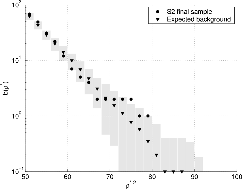
Figure 10: The number of triggers per S2 above combined SNR $\rho^{*}$ using the best-fit clustering method. The triangles represent the expected (mean) background, while the circles represent zero-shift coincident triggers. See Fig. 8 and Sec. VII for details of the time-shifts and for comparison with largest SNR clustering. We note that there is no apparent excess of S2 coincident triggers over the expected background from accidental coincidences in this plot.

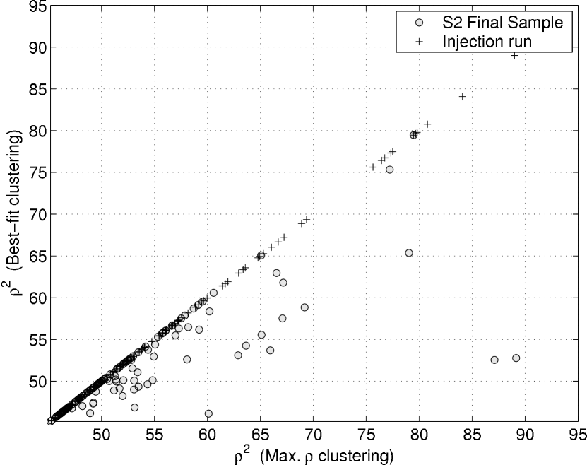
Figure 11: A comparison between the SNR associated with a cluster of triggers by maximizing the SNR over the cluster and the SNR associated with the same cluster using best-fit clustering. Notice that the best-fit clustering often gives lower SNR values for the final S2 sample, whereas simulated injections have very similar SNR values for both clustering methods. The triggers 030327, 030328, and 030224 discussed in the text are the grey circles with horizontal coordinates 89.1, 87.1 and 79.5, respectively.

IX Upper limit on the rate of coalescences per galaxy

Following the notation used in Abbott et al. (2004b), let $\mathcal{R}$ indicate the rate of binary neutron star coalescences per year per Milky Way Equivalent Galaxy (MWEG) and $N_{G}(\rho^{\ast})$ indicate the number of MWEGs to which our search is sensitive at $\rho\geq\rho^{\ast}$. The probability of observing an inspiral signal with $\rho>\rho^{\ast}$ in an observation time $T$ is

$$P(\rho>\rho^{\ast};{\mathcal{R}})=1-e^{-{\mathcal{R}}TN_{G}(\rho^{\ast})}.$$ (12)

A trigger can arise from either an inspiral signal in the data or from background. If $P_{b}$ denotes the probability that all background triggers have SNR less than $\rho^{\ast}$, then the probability of observing one or more triggers with $\rho>\rho^{\ast}$ is given by

$$P(\rho>\rho^{\ast};{\mathcal{R}},b)=1-P_{b}e^{-{\mathcal{R}}TN_{G}(\rho^{\ast})}.$$ (13)

Given the probability $P_{b}$, the total observation time $T$, the largest observed signal-to-noise $\rho_{\mathrm{max}}$, and the number of MWEGs $N_{{G}}(\rho_{\mathrm{max}})$ to which the search is sensitive, we find that the rate of binary neutron star inspirals per MWEG satisfies

$${\cal R}<{\cal R}_{90\%}=\frac{2.303+\ln P_{b}}{TN_{G}(\rho_{\mathrm{max}})}$$ (14)

with 90% confidence. This is a frequentist upper limit on the rate. For ${\mathcal{R}}>{\mathcal{R}}_{90\%}$, there is more than $90\%$ probability that at least one event would be observed with SNR greater than $\rho_{\mathrm{max}}$. Details of this method of determining an upper limit can be found in Ref. Brady et al. (2004). In particular, one obtains a conservative upper limit by setting $P_{b}=1$; we adopt this approach below because of uncertainties in our background estimate.

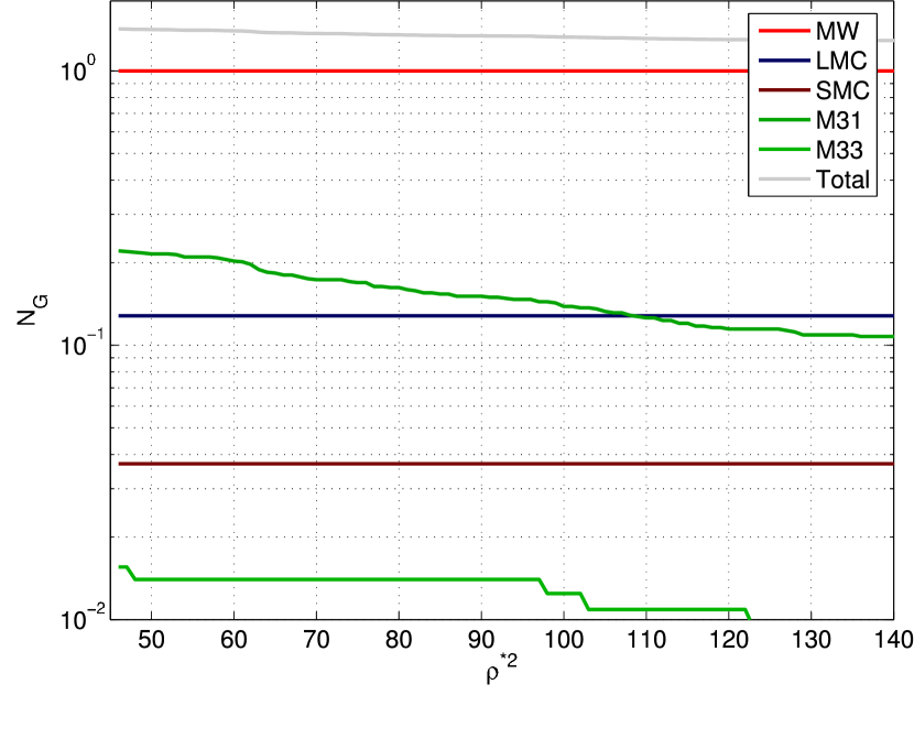
Figure 12: The efficiency of the search to the target population described in Sec. III as a function of the SNR threshold $\rho^{*}$. The contribution of each galaxy to $N_{G}$ is shown for galaxies which contribute more than $1\%$ of an MWEG. The largest SNR of a coincident trigger observed in this analysis was $\rho^{2}=89$ meaning that $N_{G}=\mbox{$1.34$}\textrm{ MWEG}$ were probed by the search.

During the $T={\color[rgb]{0,0,0}{\mbox{$339$}}}\text{ h}$ of data used in our analysis, the largest observed SNR was $\rho_{\mathrm{max}}^{2}={\color[rgb]{0,0,0}{\mbox{$89.1$}}}$. The number of MWEGs $N_{G}$ was computed using a Monte Carlo simulation in which the data was re-analyzed with simulated inspiral signals, drawn from the population described in Sec. III, added to the time series. The results are shown in Fig. 12 which breaks down the contribution to $N_{G}$ galaxy by galaxy in the target population. (Results are shown only for galaxies contributing more than 0.01 MWEG.) At $\rho^{\ast 2}={\color[rgb]{0,0,0}{\mbox{$89.1$}}}$, we find $N_{G}=\mbox{$1.34$}\textrm{ MWEG}$; this is subject to some uncertainties, to be discussed in the next section. We determine that the probability that all background events have SNR smaller than the largest observed SNR is $P_{b}={\color[rgb]{0,0,0}{0.8}}$. Since no systematic error has been assigned to this background estimate, we take $P_{b}=1$ to be conservative. As a function of the true value of $N_{\text{G}}$, the rate limit is

$${\mathcal{R}}_{90\%}=\mbox{$44.4$}\left(\frac{\mbox{$1.34$}}{N_{\text{G}}}\right)\text{ y}^{-1}\text{ MWEG}^{-1}\;.$$ (15)

IX.1 Error analysis

The principal systematic effects on our rate limit are (i) inaccuracies in our model population, including inaccuracies in the inspiral waveform assumed, and (ii) errors in the calibration of the instrument. All other systematic effects in the analysis pipeline (for example, less-than-perfect coverage of the template bank) are taken into account by the Monte Carlo estimation of the detection efficiency. It is convenient to express the effective number of MWEGs as

$$N_{\mathrm{G}} = \varepsilon(\rho_{\mathrm{max}})\left(\frac{L_{\mathrm{pop}}}{L_{\mathrm{MW}}}\right)$$ (16)

$$= \sum_{i=0}^{n}\varepsilon_{i}(\rho_{\mathrm{max}})\frac{L_{i}}{L_{MW}}$$ (17)

where $L_{\mathrm{MW}}$ is the effective blue-light luminosity of the Milky Way and the index $i$ identifies a galaxy in the population where $i=0$ corresponds to the Milky Way. The fraction of the signals that would be detectable from a particular galaxy in this search is denoted $\varepsilon_{i}$ – we will refer to this as the efficiency of the search to sources in galaxy $i$. Referring to Table 1, $\varepsilon_{i}(\rho_{\mathrm{max}})$ is given in column 6, $L_{i}/L_{\mathrm{MW}}$ in column 5, and the cumulative value of $N_{\mathrm{G}}$ in column 7.

IX.1.1 Uncertainties in population model

Uncertainties in the population model used for the Monte-Carlo simulations may lead to differences between the inferred rate and the rate in the universe. Since the effective blue-light luminosity $L_{\text{pop}}$ is normalized to our Galaxy, variations arise from the relative contributions of other galaxies in the population. These contributions depend on the estimated distances to the galaxies, estimated reddening, and corrections for metallicity (lower values tend to produce higher mass binaries), among other things.

The spatial distribution of the sources can also introduce significant uncertainties. Typically, the distances to nearby galaxies are only known to about 10% accuracy. In fact, the distance to Andromeda is thought to suffer from a $15\%$ error. A change in distance $\Delta d$ to a galaxy assumed to be at distance $d$ introduces two different uncertainties in $N_{\mathrm{G}}$:

1. The change in our estimate of the efficiency for the particular galaxy is determined by observing that the correct signal to noise ratio decreases inversely with the distance to the galaxy and hence

   $$\varepsilon_{i}(\rho_{\mathrm{max}})\rightarrow\varepsilon_{i}(\rho_{\mathrm{max}}[1+\Delta d/d])$$ (18)

   so that efficiency decreases as the distance increases.

2. The change in our estimate of the luminosity that is correlated with this change in distance is given by

   $$\frac{L_{i}}{L_{\mathrm{MW}}}\rightarrow\frac{L_{i}}{L_{\mathrm{MW}}}\left(\frac{d+\Delta d}{d}\right)^{2}$$ (19)

   so that our estimate of the luminosity increases as the distance increases.

Adopting a $15\%$ error in all distances, we estimate the error in $N_{G}$ due to uncertainties in galactic distances to be

$$\left.\delta N_{G}\right|_{d}=0.04\textrm{ MWEG}\;.$$ (20)

The absolute blue light luminosity of the Milky Way is uncertain since it is inferred from other galactic parameters. There appears to be some confusion about the this in the literature on binary neutron star rate estimates. Phinney Phinney (1991) used $L_{\mathrm{MW}}=1.6\times 10^{10}L_{\odot,B}$ while the more recent work of Kalogera, Narayan, Spergel and Taylor Kalogera et al. (2001) uses $9\times 10^{9}L_{\odot,V}$ citing a factor of two difference with the number used by Phinney; these number agree within 1%, however, once converted to the same units.

Errors in the blue magnitude of each galaxy and relative normalization to the Milky Way enter in the same way. For the galaxies that contribute most substantially to $N_{G}$, the LEDA catalog suggests errors of $\sim 10\%$ in corrected blue magnitude which translates into errors of $\sim 20\%$ in luminosity. Adopting this uniformly for the galaxies in our population, we estimate

$$\left.\delta N_{G}\right|_{L}=0.04\textrm{ MWEG}$$ (21)

Different models for NS-NS formation can lead to variations in the NS mass distribution Belczynski et al. (2002), although the bulk of the distribution always remains strongly peaked around observed NS masses Thorsett and Chakrabarty (1999). We estimate the corresponding variations in $N_{G}$ to be

$$\left.\delta N_{G}\right|_{\mathrm{mass}}\approx 0.01\textrm{ MWEG}$$ (22)

based on simulations with 50% reduction in the number of binary systems with masses in the range $1.5M_{\odot}<m_{1},m_{2}<3.0M_{\odot}$. This is indicative only. A few extreme scenarios for binary formation can produce more severe alterations to the mass distribution Belczynski et al. (2002).

The waveforms used both in the Monte-Carlo simulation and in the detection templates ignore spin effects. Estimates based on the work of Apostolatos Apostolatos (1995) suggest that less than 10% of all spin-orientations and parameters consistent with binary neutron stars provide a loss of SNR greater than $\sim 5\%$. Thus, the mismatch between the signal from spinning neutron stars and our templates should not significantly affect the upper limit. To be conservative, however, we place an upper limit only on non-spinning neutron stars; we will address this issue quantatively in future analysis.

IX.1.2 Uncertainties in the instrumental response

The uncertainty in the calibration can be quantified as an uncertainty in amplitude and phase of a frequency dependent response function.

Using the same procedure as in S1 Adhikari et al. (2003), the average instrument response $R(f)$ was constructed for every minute of data during S2 from a reference sensing function $C(f)$, a reference open loop gain function $G(f)$, and a parameter $\alpha(t)$ representing varying optical gain. The response function at a time $t$ during the run is given by $R(f,t)=(1+\alpha(t)G(f))/(\alpha(t)C(f))$. The parameter $\alpha$ was reconstructed using the observed amplitude of a calibration line. If an inspiral signal is present in the data, errors in the calibration can cause a mismatch between the template and the signal. We can quantify and measure this effect using simulated injections, both in software and hardware. For such injections, the SNR differs from the SNR that would be recorded for a signal from a real inspiral event at the same distance as the injection. The effect is linear in amplitude errors causing either an upward or downward shift in SNR; in contrast, the effect is quadratic in phase errors causing an over-estimation of sensitivity Brown (for the LIGO Scientific Collaboration). This error is propagated to our upper limit by shifting the efficiency curve in Fig. 12 horizontally by the appropriate amount.

A careful evaluation of uncertainties in the S2 calibration González et al. (2004) has shown that amplitude errors have two dominant components. The first source of error, an imperfect knowledge of the strength of the feedback actuators in the system, produces an error in the overall amplitude of the sensing function $C(f)$. Thus, it manifests as a systematic error in the amplitude of the response function, constant during the whole run. This error was estimated to be 8.5% in L1, 3.5% in H1, and 4.5% in H2.

The second dominant source of error is an imprecise measurement of the amplitude of the calibration line, resulting in an error of the coefficient $\alpha(t)$. This measurement error is mostly random in nature, and leads to magnitude and phase errors in the response function. These errors translate into maximum amplitude errors in the response function equal to 6% for L1 and H2, and 18% for H1.

Another source of error in $\alpha(t)$, which is not captured in the errors as estimated above, is due to changes in optical gain that are averaged over the 60 second integration time used in the measurement of $\alpha(t)$. Based on a limited set of diagnostics, we roughly estimate these errors can be as large as 10% in L1, and smaller in H1 and H2. The errors in $\alpha$, including these fast fluctuations, are random in nature, and are not expected to contribute to the error in the measured efficiency.

The SNR used in the final analysis is constructed from the individual SNR’s $\rho_{L}$ and $\rho_{H}$ as given in Eq. (10). The error in SNR then has two pieces

$$(\delta\rho)^{2} = \frac{\rho_{L}^{2}}{\rho^{2}}(\delta\rho_{L})^{2}+\frac{1}{4^{2}}\frac{\rho_{H}^{2}}{\rho^{2}}(\delta\rho_{H})^{2}$$ (23)

$$\leq (\delta\rho_{L})^{2}+\frac{1}{4^{2}}(\delta\rho_{H})^{2}$$ (24)

We assume fractional errors equal to the maximum errors in calibration at each site and arising from the systematic uncertainty in the detector response (8.5% in L1, and 4.5% for LHO). This results in a conservative estimate of the error at the largest observed SNR:

$$(\delta\rho)^{2}\leq(0.085\rho_{\mathrm{max}})^{2}+0.0625(0.045\rho_{\mathrm{max}})^{2}\;.$$ (25)

The resulting error on $N_{G}$ is

$$\left.\delta N_{G}\right|_{\mathrm{cal}}=0.02\textrm{ MWEG}$$ (26)

Simulations of the contributions to $\delta N_{G}$ from the random fluctuations of $\alpha$, assuming the largest possible error in H1 (18%), made negligible contributions to the error due to calibration, as expected.

IX.1.3 Uncertainties in the analysis pipeline

Since we use matched filtering to search for gravitational waves from inspiralling binaries, differences between the theoretical and the real waveforms could also adversely effect the results. These effects have been studied in great detail for binary neutron star systems Apostolatos (1995); Droz and Poisson (1997); Droz (1999). The results indicate a $\sim 10\%$ loss of SNR due to inaccurate modelling of the waveforms for binaries in the mass range of interest. This feeds into our result through our measurement of the efficiency. We may be over-estimating our sensitivity to real binary inspiral signals; the estimated loss of efficiency results in an error on $N_{G}$ of

$$\left.\delta N_{G}\right|_{\mathrm{wave}}=+0/-0.02\textrm{ MWEG}$$ (27)

The effects of discreteness of the template placement, errors in the estimates of the power spectral density $S(f)$ used in the matched filter in Eq. (3), and trends in the instrumental noise are all accounted for by the Monte-Carlo simulation. The error in the efficiency measurement due to the finite number of injections is estimated as

$$\left.\delta N_{G}^{i}\right|_{\mathrm{MC}}=L_{i}\sqrt{\varepsilon_{i}(1-\varepsilon_{i})/n^{i}}$$ (28)

where $n^{i}$ is the number of injections made for each galaxy. The total error from the Monte Carlo is

$$\left.\delta N_{G}\right|_{\mathrm{MC}}=0.02\textrm{ MWEG}$$ (29)

IX.1.4 Combined uncertainties on $N_{\text{G}}$ and the rate

Combining the errors in quadrature yields total errors

$$\left.\delta N_{G}\right|_{\mathrm{total}}=\mbox{$+$0.06$/$$-$0.07}\textrm{ MWEG}$$ (30)

To be conservative, we assume the downward excursion $N_{\mathrm{G}}=\mbox{$1.34$}-0.07=1.27\textrm{ MWEG}$ when using Eq. (15) to derive an observational upper limit on the rate of binary neutron star coalescence

$${\mathcal{R}}<\mbox{$47$}\textrm{ y}^{-1}\textrm{ MWEG}^{-1}$$ (31)

where we have used $T=\mbox{$339$}\textrm{ hr}$ and $P_{b}=1$.

X Summary and Discussion

Using data from the second LIGO science run (S2), we have significantly improved our methods and strategies to search for waveforms from inspiraling neutron stars. The search has been optimized for detecting signals, rather than for setting optimal upper limits on the rate of sources Abbott et al. (2004b). In order to increase confidence in a detection candidate, we used data only when two or more detectors are operating. We performed extensive validations of the detection efficiency of our search using software and hardware signal injections. Using these injections, we tuned the parameters in our search to take advantage of the increased reach of the detectors in the S2 run and have almost 100% efficiency for signals in the Milky Way and the Magellanic clouds. (Due to the antenna pattern, we cannot be 100% efficient.) We also achieved an average 6% efficiency for sources in the Andromeda galaxy, at a distance of 770 kpc, near the typical maximum range of our second best detector (H1, 900 kpc). Using the same detection pipeline, but shifting in time the data from the two observatories, we quantified the accidental rate for our pipeline. This allows evaluation of our confidence that any candidate is a true signal.

The search of 373 hours of double- and triple-detector data during S2 resulted in no detection: the strongest candidate from the search, arising from coincidence between L1 and H2, had a combined signal-to-noise of 9.4. Our background estimate suggests that noise has a 20% probability of causing a candidate with this signal-to-noise or greater. Moreover, the weight of evidence from follow-up investigations suggests that this trigger originated with a burst of noise which corresponded to a brief period of servo instability. The detailed investigations presented in Sec. VIII exemplify typical follow-up of coincident triggers which appear unlikely to arise from background. We have found no evidence of a gravitational wave event from binary neutron star inspiral. Without a detection, the 339 hours of non-playground data were used to place an upper limit on the rate of binary neutron star coalescence in the Universe.

This search was sensitive to binary inspiral signals from neutron star coalescence in the Local Group and other galaxies at distances of up to about 1.5 Mpc. We used Monte Carlo simulations to measure the efficiency of our search to non-spinning neutron stars in this population. We conclude that the rate of binary neutron star coalescence is $\cal{R}\leq{\mbox{$47$}}~{}{\rm yr^{-1}MWEG^{-1}}$ with 90% confidence. This rate limit is significantly greater than astrophysically plausible rates Kalogera et al. (2004), but it illustrates the performance of the search. It should be noted that the analysis of the first science run Abbott et al. (2004b) was optimized to yield the lowest upper limit, while the method presented here was not. In particular, the decision to only use data when the Livingston interferometer and one of the Hanford interferometers were operating limited the observation time to 1/3 of the total data collected. Analysis of the remaining data collected in coincidence with TAMA will be reported elsewhere Abbott et al. (2005c).

In this paper, we have presented a data analysis strategy that could lead to a detection of gravitational waves from binary neutron star inspirals. The methods used to validate the search illustrate the subtleties of the analysis of several detectors with different sensitivities and orientations. Moreover, the experience gained by following up the largest coincident triggers will be crucial input to investigations of event candidates that are identified in future searches.