ACTIVE MASS UNDER PRESSURE

Abstract

After a historical introduction to Poisson’s equation for Newtonian gravity, its analog for static gravitational fields in Einstein’s theory is reviewed. It appears that the pressure contribution to the active mass density in Einstein’s theory might also be noticeable at the Newtonian level. A form of its surprising appearance, first noticed by Richard Chase Tolman, was discussed half a century ago in the Hamburg Relativity Seminar and is resolved here.

1 Historical Introduction

By “active” mass one means the mass considered as source of a gravitational field. This concept can be distinguished from that of the “passive” mass measuring the response to a gravitational field and of an “inertial” mass describing resistance against acceleration by any force, gravitational or other. These distinctions are useful for considering non-Newtonian or non-Einsteinian theories of gravity, or to assess which aspects of mass are tested in experiments. In Newton’s and Einstein’s theories these distinctions are not necessary, in agreement with available physical and astronomical evidence and post-Newtonian approximations.

Joseph Louis Lagrange in his 1773 “Memoir on the secular Equation of the Moon” [1] introduced the function $V$ through the equation

$$V(\vec{x})=\int\frac{\rho(\vec{x^{\prime}})}{|\vec{x}-\vec{x^{\prime}}|}d^{3}\vec{x^{\prime}}.$$ (1.1)

He recognized that it is easier to first compute $V$ and then to get the accelerations by differentiation than to calculate the accelerations directly.

The function $\rho(\vec{x^{\prime}})$ denotes here the density of the active mass. The active mass is then given by

$$M=\int\rho(\vec{x^{\prime}})d^{3}\vec{x^{\prime}}.$$ (1.2)

Lagrange did not use vector notation and did not exhibit Newton’s gravitational constant $G$ because astronomers set it equal to one as we do in this paper. We recognize now Lagrange’s function $V$ as the negative of the gravitational potential $\phi$. The use of the negative of the potential was customary before the principle of the conservation of energy began to dominate physics and astronomy.

Lagrange did not supply a name for his function $V$. Carl Friedrich Gauss called it the potential in his 1839 paper on “General Theorems about Forces of Attraction and Repulsion depending on the inverse Square of the Distance” [2]. Gauss had not been aware of George Green’s 1828 article “An Essay on the Application of Mathematical Analysis on the Theory of Electricity and Magnetism” [3] that had named $V$ the “potential function”. Green had published his paper privately and had rarely referred to it in his later papers. It was only several years after Green’s death in 1841 that William Thomson (the later Lord Kelvin) discovered Green’s paper and arranged for the publication of its results.

The acceleration vector $\ddot{\vec{x}}$ for a massive particle was given by Lagrange in an inertial system by

$$\ddot{\vec{x}}=\bigtriangledown V.$$ (1.3)

This law may be read as saying that the inertial mass may be identified with the passive gravitational mass.

In his 1782 “Theory of the attraction of spheroids and the figure of the earth” [4] Pierre Simon Laplace introduced for the function $V$ the equation

$$\bigtriangledown^{2}V\equiv\frac{\partial^{2}V}{\partial x^{2}}+\frac{\partial^{2}V}{\partial y^{2}}+\frac{\partial^{2}V}{\partial z^{2}}=0$$ (1.4)

that is now named the Laplace equation. Laplace did not write it, as we just did, in Cartesian coordinates $x,y,z$ but used spherical polar coordinates. He published the form in Cartesian coordinates in his “Memoir about the theory of Saturn’s ring” [5] in 1787.

It was only 26 years later that Siméon-Denis Poisson pointed out in his “Remarks about an equation that occurs in the theory of attraction of spheroids” that the Laplace equation does not hold within the substance of the attracting body [6] and has there to be replaced by

$$\bigtriangledown^{2}V=-4\pi\rho.$$ (1.5)

This equation is now known as the Poisson equation. A proof was first given by Gauss in 1839 [2]. If we write the equations in terms of the potential $\phi$ we have

$$\bigtriangledown^{2}\phi=4\pi\rho,$$ (1.6)

the relation between the gravitational potential and the density of the active mass in an inertial system of Newton’s theory. If $\phi$ is required to vanish at infinity, (1.6) implies (1.1).

2 Static Fields in Einstein’s Theory of Gravitation

In General Relativity [7] the ten components $g_{\mu\nu}$ of the metric tensor

$$ds^{2}=g_{\mu\nu}(x^{\lambda})dx^{\mu}dx^{\nu}$$ (2.1)

replace the potential of Lagrange. Moreover, not just the mass-density, but all ten components of the energy-momentum-stress tensor $T_{\mu\nu}$ become contributing sources to the gravitational field. For neutral matter $T_{\mu\nu}$ is given by

$$T_{\mu\nu}=\rho u_{\mu}u_{\nu}+p_{\mu\nu}$$ (2.2)

with energy density $\rho$, pressure tensor $p_{\mu\nu}$ and four-velocity $u^{\mu}$ subject to the normalisation

$$u^{\mu}u_{\mu}=1,$$ (2.3)

and

$$p_{\mu\nu}u^{\nu}=0.$$ (2.4)

For a perfect fluid

$$p_{\mu\nu}=p(u_{\mu}\,u_{\nu}-g_{\mu\nu}).$$ (2.5)

Instead of Poisson’s equation relating the gravitational potential to the active mass density $\rho$ we have now the Einstein field equations

$$R_{\mu\nu}-\frac{1}{2}g_{\mu\nu}R+\lambda g_{\mu\nu}=-8\pi T_{\mu\nu}$$ (2.6)

connecting the $g_{\mu\nu}$ and their derivatives up to the second order to the components of $T_{\mu\nu}$. The Riemann tensor is defined through the interchange of order in the second covariant derivatives of a covariant vector field $\xi_{\mu}$

$$\xi_{\mu;\alpha;\nu}-\xi_{\mu;\nu;\alpha}=-\xi_{\gamma}R^{\gamma}{}_{\mu\alpha\nu}$$ (2.7)

and the Ricci tensor by

$$R_{\mu\nu}=R^{\gamma}{}_{\mu\gamma\nu}.$$ (2.8)

The Ricci scalar $R$ is obtained through contraction from the Ricci tensor $R^{\mu}{}_{\nu}$.

Here we use units where the speed of light “c” is put equal to 1.

For a static gravitational field in which the matter is at rest we are able to find an analog of Lagrange’s potential and its Poisson equation. In section 8 we give an invariant derivation of the necessary developments. Here we give just the results. A static gravitational field can be described by the metric

$$ds^{2}=g_{00}(x^{l})(dx^{0})^{2}+g_{jk}(x^{l})dx^{j}dx^{k}$$ (2.9)

with no $g_{0i}$ terms. Latin indices run here from 1 to 3. The components of the metric tensor do not depend on the time coordinate $t=x^{0}$ and the four- velocity $u^{\mu}$ of the matter is given by

$$u^{\mu}=\frac{1}{\sqrt{g_{00}}}\,\delta^{\mu}_{0}.$$ (2.10)

We have then for the static potential $\sqrt{g_{00}}$ with $\hat{g}=\det\parallel g_{jk}\parallel$

$$-\frac{1}{\sqrt{-\hat{g}}}\Big{(}\sqrt{-\hat{g}}\,g^{jk}\,(\sqrt{g_{00}})_{,k}\Big{)}_{,j}\equiv\bigtriangledown^{2}\sqrt{g_{00}}=4\pi\sqrt{g_{00}}\Big{(}\rho+3p-\frac{\lambda}{4\pi}\Big{)}.$$ (2.11)

The spatial metric differs from the flat metric only by terms of order $\phi$, On the left-hand side of the relativistic Poisson equation we have the Laplace operator on the spaces t = const. for the function $\sqrt{g_{00}}$ that we now identify as the static relativistic potential. This expression in Riemannian geometry was derived by Eugenio Beltrami in his 1868 paper “On the general theory of differential parameters” and became known as the second Beltrami parameter [8].

The cosmological term in (2.6) can be put on the right-hand side of the equation as

$$-\lambda g_{\mu\nu}\equiv-8\pi T_{\mu\nu}(\lambda),$$ (2.12)

Interpreted as an energy-momentum tensor of a perfect fluid

$$T_{\mu\nu}(\lambda)=[\rho(\lambda)+p(\lambda)]u_{\mu}u_{\nu}-p(\lambda)g_{\mu\nu}$$ (2.13)

we have

$$\rho(\lambda)=-p(\lambda),\quad p(\lambda)=-\frac{\lambda}{8\pi}.$$ (2.14)

The contribution to the active mass density (“dark energy”) becomes

$$\rho(\lambda)+3p(\lambda)=-\frac{\lambda}{4\pi}.$$ (2.15)

On the right-hand side we have Poisson’s $4\pi\rho$ term. Apart from Einstein’s lambda term that acts now–if positive–as a negative mass density contributing to the active mass, we have two changes in comparison with Poisson’s equation. One is the factor $\sqrt{g_{00}}$ on the right hand side of the equation. Since the discovery of energy conservation the potential had been defined as the work to displace a unit mass (charge) from infinity and it was usually normalized to vanish at spatial infinity. In Einstein’s theory of gravitation the component $g_{00}$ for a finite mass distribution in a static gravitational field is usually taken as $c^{2}$ or 1 at infinity. The reason is that now one includes the rest energy of a particle as part of the potential energy and assumes that the metric of an isolated system becomes Euclidean at large distances. We have then for $\sqrt{g_{00}}$ at large distances $r$ from the center of mass

$$\sqrt{g_{00}}(r)\approx 1-\frac{M}{r}$$ (2.16)

where $M$ is the total active mass. Thus, for weak fields the factor $\sqrt{g_{00}}$ in the relativistic Poisson equation differs from 1 only slightly.

The most surprising correction to the relativistic Poisson equation is the term $3p$ that is actually $3p/c^{2}$. This term was first noted explicitly as a consequence of Einstein’s field equations by Tullio Levi-Civitá in 1917 in his series of papers on “Einstein’s Static” [9]. It is this term that we shall discuss in other sections of this paper. Finally, $\sqrt{\hat{g}}\,d^{3}\vec{x^{\prime}}$ in the formula for the active mass is the proper volume element.

The justification for identifying $\sqrt{g_{00}}$ with the relativistic global potential rests on its definition as the specific potential energy. We shall show in section 11 that the test particle of unit mass resting at $\vec{x}$ has potential energy (apart from its rest-energy)

$$\phi=\sqrt{g_{00}}-1.$$ (2.17)

The Poisson equation in Newtonian gravity is written down in a global inertial system. The closest analog to such a system for Einstein’s static gravitational fields (without cosmological constant) is based on the coordinates adapted to the time-like hypersurface-orthogonal Killing vector. It also defines a rest system through the divergence-free time-like unit vectors orthogonal to the hypersurfaces t = const. reaching out to spatial infinity where the space-time metric is assumed to become Minkowskian. These coordinates, it has to be stressed, are not local inertial systems. The acceleration of a particle at rest is given by

$$\dot{u}_{k}=-\,\frac{1}{\sqrt{g_{00}}}\frac{\partial}{\partial x^{k}}\sqrt{g_{00}}=-\frac{\phi_{,k}}{(1+\phi)}.$$ (2.18)

3 Tolman’s Paradox

Richard Chase Tolman in his 1930 paper “On the use of the energy-momentum principle in general relativity” [10] derived a formula for the total energy of a fluid sphere in a quasi-static state for Einstein’s theory of gravitation. He wrote with a proper volume element $dV_{0}$

$$M=\int(\rho+3p)\sqrt{g_{00}}\,dV_{0}=\int\partial_{a}\phi\,d\vec{F}^{a}$$ (3.1)

suppressing the cosmological term, where $\rho$ is the relativistic energy density.

In statistical mechanics of an ideal gas consisting of particles with mass $m$, and momentum $\vec{p}$, velocity $\vec{v}$, and number density $n$, the pressure $p$ is given by Daniel Bernoulli’s formula [11] from his 1738 “Hydrodynamics, commentaries about forces and motions in fluids”

$$p=\frac{1}{3}\overline{n\,\vec{p}\cdot\vec{v}}$$ (3.2)

where the bar indicates averaging. In (3.2) $p$ is the kinetic contribution to the pressure. In general $p$, or $p_{jk}$ contains contributions from short-range interactions, which have to be added to (3.2). Attractive interactions contribute negative $p$. This formula, as written above, holds also for a relativistic ideal gas as discussed by Franz Juettner in his paper on “Maxwell’s law of velocity distribution in the relative theory”[12]. In the high energy limit of photons with energy $\epsilon$ this gives

$$\vec{p}\cdot\vec{v}=\epsilon,\quad p=\frac{1}{3}\overline{n\,\epsilon}=\frac{1}{3}\rho.$$ (3.3)

Since Tolman was particularly interested in the “gravitational mass of disordered radiation,” the $3p$-term in the active mass density caught his attention. This was no longer one of the tiny effects of general relativity. Tolman’s observation led to the following paradox: while matter at rest in a spherical container of negligible matter might exhibit a total mass $M$ in the far field of the container, transformation of the mass inside the container into disordered radiation would then double the total mass violating the conservation of $M$. After the discovery of the positron in 1932 and its annihilation with the electron such complete transformations of matter into radiation were no longer impossible.

4 The Hamburg paradox

The authors of this paper were members of a seminar on relativity that regularly met at Hamburg University in the 1950’s. When we learned about the $3p$-term in the Poisson equation the following test was suggested:

Since nucleons move in atomic nuclei with about two tenths of the speed of light, the $3p$-term might significantly contribute to the active mass density of all nuclei except hydrogen and the neutron. A simple calculation for the pressure in an ideal Fermi gas of nucleons at zero temperature (see section 13) gave a pressure contribution to the active mass density of 4.3 % for nuclear matter. A ball of hydrogen should, therefore, have an active mass about 4 % smaller then a ball of lead of the same inertial and passive gravitational mass that could be checked by weighing them on scales.

However, the only way such an effect might be seen in the laboratory was by the Cavendish experiment for the determination of the gravitational constant where the active mass came into play. While it would be forbidding to work with a ball of ultra-cold solid hydrogen one might consider a material with a high hydrogen content that was solid at room temperature like polyethylene of formula $CH_{2}$ or lithium hydride of formula $LiH$.

For lithium hydride we have

$$0.043/8=5\times 10^{-3}$$ (4.1)

and for polyethylene

$$2\times 0.043/14=6\times 10^{-3}.$$ (4.2)

If one were to use balls of these materials for a determination of the gravitational constant through the Cavendish experiment one should thus get lower values for the gravitational constant $G$. In the fifties the value of $G$ was uncertain by about 0.1 % [13] and so the effect might just be measurable. When one of us (ELS) talked in 1958 to Robert Dicke of Princeton University about a possible experimental test Dicke had his doubts whether it could be done since machining homogeneous spheres in those materials might be forbidding. However, a year later it became clear that there should be no different value for $G$ with balls of hydrogen. Dieter Brill from Princeton who had joined the Hamburg seminar alerted us to a paper in the Physical Review by Charles Misner and Peter Putnam [14] about active mass (about Peter Putnam who died in 1987 see John Wheeler’s Memoir [15].)

Misner and Putnam showed, assuming gravity to be negligible, that the 3p-term for a gas in a container was canceled by negative contributions to the mass from the stresses in the walls of the container that kept the gas together. It had not been clear to us that negative surface contributions to the energy would exactly cancel the positive 3p-volume contribution to the total mass when we had the model of a bubble in mind.

5 The spherical bubble

We imagined a gas of constant density $\rho$ and pressure $p$ enclosed in a spherical two-dimensional shell of radius $r$ with surface mass density $\sigma$ and surface tension $\tau$.

Figure 1: A spherical bubble of radius $r$ is filled with a gas of pressure $p$. The bubble is kept in equilibrium by a surface tension $\sigma$ with dimension force by length.

The surface tension should be just strong enough for keeping the bubble in equilibrium. The gravitational binding energy of the bubble was supposed to be negligible compared to its mass. For finding the relation of surface tension to pressure for equilibrium we imagined a plane cut through the bubble removing the southern hemisphere. To keep the northern hemisphere in equilibrium one now had to balance the upward pressure over the equatorial disc of area $\pi r^{2}$ against the surface tension pulling down along the equator over the length $2\pi r$. This gives the relation

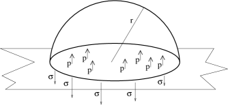
Figure 2: The lower hemisphere of the bubble (Fig.1) is removed and replaced by its forces on the upper hemisphere.

$$p\cdot\pi r^{2}=\tau\cdot 2\pi r,\quad\tau=\frac{1}{2}p\,r.$$ (5.1)

The total active mass $M$ would then be obtained by the surface contribution $4\pi r^{2}(\sigma-\tau)$ and by the volume contribution $4\pi r^{3}(\rho+3p)/3$

$$M=4\pi r^{2}(\sigma-\tau)+\frac{4\pi}{3}r^{3}(\rho+3p)=4\pi r^{2}\sigma+\frac{4\pi}{3}r^{3}\rho+2\pi r^{3}p$$ (5.2)

leaving us with half the volume contribution of the $3p$-term to the active mass. Something was wrong. It was only last summer in a nostalgic moment when we talked about this problem again that we saw the solution:

If the active mass density of a 3-dimensional distribution has to be complemented by a $3p$-term, then that of a 2-dimensional shell needs a $2p$-term and a 1-dimensional disk a $p$-term (corresponding to the trace of a 2- or 1-dimensional isotropic stress tensor) If they were stresses instead of pressures they would come in with a negative sign.

Now all was clear: the surface contribution to the active mass of the bubble was $4\pi r^{2}(\sigma-2\tau)$ and we obtain now instead (5.2)

$$M=4\pi r^{2}(\sigma-2\tau)+\frac{4\pi}{3}r^{3}(\rho+3p)=4\pi r^{2}\sigma+\frac{4\pi}{3}r^{3}\rho.$$ (5.3)

This simple remark settled also the case of the active mass of a circular disk.

6 The active mass of a circular disk

We consider a circular disk of radius $r$ with mass density $\sigma$ and pressure $p$

Figure 3: Circular disk of radius $r$ carries a surface pressure $p$ with dimension force/length. The Pressure is balanced by the tension $\lambda$ with dimension force along its perimeter.

The disk is kept in equilibrium by a one-dimensional string around its circumference of linear mass density $\mu$ and stress $\lambda$. To find the relation between the pressure $p$ and the stress $\lambda$ we imagine a linear cut through the center of the disk removing the lower half

Figure 4: The lower half of the disk (Fig. 3) has been removed and replaced by the forces acting on the upper part.

The pressure over the diameter $2r$ must now be balanced against the stress $\lambda$ at the left and the right end of the semicircle. This gives

$$2r\,p=2\lambda,\quad\lambda=r\,p.$$ (6.1)

The active mass $M$ of the disk is then obtained by taking the active mass density $\sigma+2p$ over the area $\pi r^{2}$ and adding the active mass density $\mu-\lambda$ of the bounding string along the circumference $2\pi r$. This gives

$$M=(\sigma+2p)\pi r^{2}+(\mu-\lambda)2\pi r=\sigma\pi r^{2}+\mu\cdot 2\pi r,$$ (6.2)

the promised result.

7 Conclusion

In Newtonian theory there was always the understanding, because of “actio = reactio”, that the active and passive masses were equal. If this were not the case a system of two passive unit masses but different active masses would show an acceleration of its center of mass violating Newton’s law actio = reactio. In Einstein’s theory of gravitation the equality of active and passive mass is not so obvious since Einstein’s cosmological constant can be seen as giving rise to self-acceleration for the center of mass of a double star. While we have no reason to doubt the equality of the three kinds of masses we believe that tests involving the active mass are certainly desirable. This is especially true for situations where the gravitational binding energy significantly contributes to the mass.

In General Relativity the fundamental variables are “local” ones, such as $g_{\alpha\beta}$, $T^{\alpha\beta}$, $\rho$, $u^{\alpha}$, $p$ …neither the active nor the passive or the inertial mass of an (extended) body have been exactly defined so far, these concepts belong to perturbative theories in General Relativity.

8 Killing’s Equation

A stationary gravitational field is characterized by the existence of a time-like Killing field that generates an infinitesimal transformation that leaves the metric unchanged. The field is called static if the Killing vector field is hypersurface-orthogonal; this means the covariant vector is a product of a gradient by a scalar function. A Killing vector field $\xi_{\mu}$ fulfills the equation

$$\xi_{\mu;\nu}+\xi_{\nu;\mu}=0.$$ (8.1)

If we write down equation (2.5) three times with cyclic permutation of the indices

$$\xi_{\mu;\alpha;\nu}-\xi_{\mu;\nu;\alpha}=-\xi_{\gamma}R^{\gamma}{}_{\mu\alpha\nu},$$ (8.2)

$$\xi_{\alpha;\nu;\mu}-\xi_{\alpha;\mu;\nu}=-\xi_{\gamma}R^{\gamma}{}_{\alpha\nu\mu},$$ (8.3)

$$\xi_{\nu;\mu;\alpha}-\xi_{\nu\alpha;\mu}=-\xi_{\gamma}R^{\gamma}{}_{\nu\mu\alpha},$$ (8.4)

adding the first two equations and subtracting the third, we have because of (8.1) and the cyclic symmetry of the Riemann tensor

$$R^{\gamma}{}_{\mu\alpha\nu}+R^{\gamma}{}_{\alpha\nu\mu}+R^{\gamma}{}_{\nu\mu\alpha}=0$$ (8.5)

that

$$2\,\xi_{\mu;\alpha;\nu}=2\,\xi_{\gamma}R^{\gamma}{}_{\nu\mu\alpha}.$$ (8.6)

These equations are known as the integrability conditions for the Killing field. If we define

$$\xi_{\mu;\alpha}-\xi_{\alpha;\mu}=2\,\xi_{\mu;\alpha}\equiv F_{\mu\alpha}\quad\text{and}\quad 2\,\xi_{\gamma}R^{\gamma}{}_{\mu}\equiv j_{\mu},$$ (8.7)

we obtain from (8.6) by anti-symmetrization and contraction Maxwell’s equations for a field tensor $F_{\mu\nu}$ and a four-current $j_{\mu}$

$$F_{\mu\alpha;\nu}+F_{\alpha\nu;\mu}+F_{\nu\mu;\alpha}=0,\quad F^{\mu\nu}{}_{;\nu}=j^{\mu}.$$ (8.8)

Since

$$\xi_{\mu;\alpha}-\xi_{\alpha;\mu}=\xi_{\mu,\alpha}-\xi_{\alpha,\mu}=F_{\mu\alpha}$$ (8.9)

the Killing vector for a stationary gravitational field plays the rôle of an electromagnetic four-potential.

9 Adapted Coordinates

We choose coordinates in such a way that

$$\xi^{\mu}=\delta^{\mu}_{0}.$$ (9.1)

That can be done for any contravariant vector field in a finite region. This specialization still allows gauge transformation with an arbitrary function $\chi(x^{k})$

$$\bar{x}^{0}=x^{0}+\chi(x^{k}),\quad d\bar{x}^{0}=dx^{0}+\chi_{,j}\,dx^{j},\quad\bar{x}^{j}=\bar{x}^{j}(x^{k}).$$ (9.2)

The Killing equation (8.1) can be written

$$g_{\mu\nu,\lambda}\xi^{\lambda}+g_{\lambda\nu}\xi^{\lambda}{}_{,\mu}+g_{\mu\lambda}\xi^{\lambda}{}_{,\nu}=0.$$ (9.3)

This gives with our normalization (9.1)

$$g_{\mu\nu,0}=0,$$ (9.4)

that is independence of the coordinate $x^{0}$. Since we requested that the Killing vector $\xi^{\mu}$ be time-like we have that $x^{0}$ is a distinguished time coordinate with

$$\xi_{\mu}=g_{0\mu},\quad\xi^{\mu}\xi_{\mu}=g_{00}>0.$$ (9.5)

Using now the condition that the Killing vector is hypersurface-orthogonal (static field)

$$\xi_{\mu}(\xi_{\nu,\lambda}-\xi_{\lambda,\nu})+\xi_{\nu}(\xi_{\lambda,\mu}-\xi_{\mu,\lambda})+\xi_{\lambda}(\xi_{\mu,\nu}-\xi_{\nu,\mu})=0$$ (9.6)

we have after contraction with $\xi^{\mu}$,

$$g_{00}(g_{0\nu,\lambda}-g_{0\lambda,\nu})-g_{0\nu}\,g_{00,\lambda}+g_{0\lambda}\,g_{00,\nu}=0.$$ (9.7)

This gives after division by $(g_{00})^{2}$

$$(g_{0\nu}/g_{00})_{,\lambda}-(g_{0\lambda}/g_{00})_{,\nu}=0.$$ (9.8)

We have, therefore, that $g_{0\nu}/g_{00}$ is a gradient of a scalar function $\psi$

$$g_{0\nu}=g_{00}\psi_{,\nu},\quad\psi_{,0}=1.$$ (9.9)

We can write

$$d\psi=dx^{0}+\psi_{,j}(x^{k})\,dx^{j}.$$ (9.10)

Comparison with (9.2) shows that we can choose the gauge transformation $\chi$ such that

$$\psi=\bar{x}^{0}.$$ (9.11)

By dropping the bar on $\bar{x}^{0}$ we have then for the metric the form (2.8)

$$ds^{2}=g_{00}(x^{l})\,(dx^{0})^{2}+g_{jk}(x^{l})\,dx^{j}dx^{k}.$$ (9.12)

The purely spatial coordinate transformations are still free. The time-like hypersurface-orthogonal Killing vector is, in general, unique up to a constant factor. The square of this factor multiplies $g_{00}$.

10 Poisson Equation

The length of the Killing vector is $\sqrt{g_{00}}$. A state of rest is then desribed by a time-like unit vector

$$u^{\mu}=\frac{1}{\sqrt{g_{00}}}\xi^{\mu},\quad u^{\mu}u_{\mu}=1.$$ (10.1)

We study now the second set of Maxwell’s equations (8.8) in adapted coordinates. We have because of time independence

$$F^{\mu\nu}{}_{;\nu}=\frac{1}{\sqrt{-g}}\Big{(}\sqrt{-g}F^{\mu\nu}\Big{)}_{,\nu}=\frac{1}{\sqrt{-g}}\Big{(}\sqrt{-g}F^{\mu k}\Big{)}_{,k}.$$ (10.2)

Since by (8.7)

$$F_{\mu\nu}=\Big{(}g_{00}\delta^{0}_{\mu}\Big{)}_{,\nu}-\Big{(}g_{00}\delta^{0}_{\nu}\Big{)}_{,\mu},$$ (10.3)

the only non-vanishing covariant components are

$$F_{0j}=g_{00,j}=-F_{j0}.$$ (10.4)

Entered into (10.2) this gives

$$F^{\mu\nu}{}_{;\nu}=\delta^{\mu}_{0}\frac{1}{\sqrt{-g}}\Big{(}\sqrt{-g}\,g_{00,j}\,\frac{1}{g_{00}}\,g^{jk}\Big{)}_{,k}$$ (10.5)

with

$$\sqrt{-g}=\sqrt{g_{00}}\sqrt{-\hat{g}},\quad\hat{g}=\det\parallel g_{jk}\parallel.$$ (10.6)

We obtain

$$F^{\mu\nu}{}_{;\nu}=\delta^{\mu}_{0}\frac{2}{\sqrt{-g}}\Big{(}\sqrt{-\hat{g}}\,g^{jk}(\sqrt{g_{00}})_{,j}\Big{)}_{,k}=-\frac{2}{\sqrt{g_{00}}}\delta^{\mu}_{0}\bigtriangledown^{2}\sqrt{g_{00}}.$$ (10.7)

The four-current $j_{\mu}$ from (8.7) becomes with the Einstein field equations (2.4)

$$j_{\mu}=2\,\xi_{\gamma}R^{\gamma}{}_{\mu}=2\Big{(}-\kappa T^{\gamma}{}_{\mu}+\frac{1}{2}\,\delta^{\gamma}{}_{\mu}\,\kappa\,T+\lambda\,\delta^{\gamma}{}_{\mu}\Big{)}\xi_{\gamma}$$ (10.8)

or

$$j^{\mu}=2\Big{(}-\kappa\,T^{\mu}_{0}+\frac{1}{2}\,\delta^{\mu}_{0}\,(\kappa\,T+2\lambda)\Big{)}.$$ (10.9)

Here $T$ is the trace (contraction) of the tensor $T^{\mu}{}_{\nu}$. The second set of Maxwell’s equations state that

$$T_{0}{}^{j}=0$$ (10.10)

saying that the density of momentum and energy flux vanish in this static situation. Calling the energy density $\rho$ and the trace of the pressure tensor $3p$

$$T=\rho-3p,\quad\rho\equiv T^{0}{}_{0},\quad 3p=-T^{a}{}_{a}$$ (10.11)

we have

$$j^{0}=-\kappa\,(\rho+3p)+2\lambda.$$ (10.12)

With (10.7) this gives the relativistic Poisson equation for a static gravitational field.

$$\bigtriangledown^{2}\sqrt{g_{00}}=\sqrt{g_{00}}\Big{(}4\pi(\rho+3p)-\lambda\Big{)}.$$ (10.13)

11 The energy of a particle in a static gravitational field

A particle of constant mass $m$ and four-velocity $v^{\mu}$ moving on a geodesic in a static gravitational field obeys

$$v^{\mu}v_{\mu}=1,\quad\dot{v}^{\mu}\equiv v^{\mu}{}_{;\nu}v^{\nu}=0.$$ (11.1)

The energy integral for unit mass is given by

$$E=v^{\mu}\,\xi_{\mu}$$ (11.2)

since

$$\dot{E}=(v^{\mu}\,\xi_{\mu})^{\dot{}}=v^{\mu}{}_{;\nu}v^{\nu}\,\xi_{\mu}+\xi_{\mu;\nu}v^{\mu}\,v^{\nu}=0.$$ (11.3)

The first term on the right hand side vanishes because of the geodesic equation (11.1) while the second term is zero due to the Killing equation (8.1).

In terms of the components of the local rest frame we have

$$E=\frac{m}{\sqrt{1-\beta^{2}}}\,\sqrt{g_{00}}$$ (11.4)

where $\beta$ is the local velocity in terms of the speed of light.

12 Acceleration of a particle at rest

A particle at rest is characterised by its four-velocity

$$u_{\mu}=\frac{1}{\sqrt{g_{00}}}\,\delta^{0}_{\mu}$$ (12.1)

The acceleration of the particle is given by

$$\dot{u}_{\mu}\equiv u_{\mu;\nu}\,u^{\nu}=u_{\mu,\nu}\,u^{\nu}-\Gamma_{\mu\nu}{}^{\lambda}u_{\lambda}u^{\nu}$$ (12.2)

Since $g_{00}$ is independent of time the first term on the right-hand side vanishes. We obtain then with (12.1)

$$\dot{u}_{\mu}=-\Gamma_{\mu\nu}{}^{\lambda}u_{\lambda}u^{\nu}=-\frac{1}{g_{00}}\,\Gamma_{\mu 0,0}=-\frac{1}{2\,g_{00}}\,g_{00,\mu}$$ (12.3)

or

$$\dot{u}_{k}=-\frac{1}{2\,g_{00}}\,g_{00,k}=-\frac{(\sqrt{g_{00}})_{,k}}{\sqrt{g_{00}}}.$$ (12.4)

13 The pressure of an ideal Fermi gas at zero temperature

The pressure for such a gas at zero temperature was derived by Enrico Fermi in his 1926 paper “On the quantization of the ideal mono-atomic gas” [16]. For $N$ identical particles in volume $V$ we have a number density $n=N/V$ and according to (3.1)

$$p\,V=\frac{1}{3}\,N\,\overline{\vec{p}\cdot\vec{v}}.$$ (13.1)

For a non-relativistic motion this gives with a mass $m$

$$p\,V=\frac{N}{3}\,\overline{(\vec{p})^{2}}/m=\frac{2}{3}N\,\bar{\epsilon}$$ (13.2)

where $\bar{\epsilon}$ is their average kinetic energy.

For an ideal Fermi gas at zero temperature in a cubic box of side length $L$ for a statistical weight $g$ we can fit $g$ particles in a cell of phase space of size

$$L^{3}\cdot\triangle p_{x}\cdot\triangle p_{y}\cdot\triangle p_{z}=h^{3}.$$ (13.3)

While Fermi took $g=1$, the case of general $g$ was discussed by Wolfgang Pauli in his 1927 paper “On gas degeneration and paramagnetism” [17].

We have thus for $dN$ particles

$$dN=g\cdot 4\pi\,(\vec{p})^{2}d|\,\vec{p}\,|\Big{(}\frac{L}{h}\Big{)}^{3}$$ (13.4)

and for the total number $N$ of particles in terms of the maximum Fermi momentum $P_{F}$

$$N=g\frac{4\pi}{3}\Big{(}\frac{P_{F}\cdot L}{h}\Big{)}^{3},\quad n=\frac{N}{V}=g\frac{4\pi}{3}\Big{(}\frac{P_{F}}{h}\Big{)}^{3}.$$ (13.5)

We obtain the average kinetic energy by averaging the expression $(\vec{p})^{2}/2m$ and obtain

$$\bar{\epsilon}=\frac{1}{N}\int\frac{(\vec{p})^{2}}{2m}dN=\frac{3}{2mp_{F}^{3}}\int\limits^{P_{F}}_{0}(\vec{p})^{4}d|\,\vec{p}\,|=\frac{3P_{F}^{2}}{10m}.$$ (13.6)

This gives for the pressure from (13.2)

$$p=\frac{n}{5m}P_{F}^{2}.$$ (13.7)

The ratio of $3p/c^{2}$ to the mass density $\rho$ becomes

$$\frac{3p}{\rho c^{2}}=\frac{3}{5}\Big{(}\frac{P_{F}}{mc}\Big{)}^{2}$$ (13.8)

The equation (13.5) allows us to express the Fermi momentum in terms of the particle density and we obtain thus

$$P_{F}=h\Big{(}\frac{3n}{4\pi g}\Big{)}^{1/3}.$$ (13.9)

Substituting this expression into (13.8) gives

$$\frac{3p}{\rho c^{2}}=\frac{3}{5}\Big{(}\frac{h}{mc}\Big{)}^{2}\Big{(}\frac{3n}{4\pi g}\Big{)}^{2/3}$$ (13.10)

or in terms of Dirac’s $\hbar$

$$\frac{3p}{\rho c^{2}}=\frac{3}{5}\Big{(}\frac{\hbar}{mc}\Big{)}^{2}\Big{(}\frac{6\pi^{2}n}{g}\Big{)}^{2/3}.$$ (13.11)

14 The atomic nucleus as a degenerate Fermi gas

Werner Karl Heisenberg considered an atomic nucleus as a Fermi gas of nucleons in his 1933 paper [18] “On the Structure of atomic nuclei III”. We want to calculate the term $3p/c^{2}\rho$ for an ideal Fermi gas of nucleons at zero temperature.The interactions among nucleons that keep them confined are simply taken into account by a potential well in which they move freely. For a rough estimate we disregard the difference between protons and neutrons and take the statistical weight $g$ to be

$$g=4.$$ (14.1)

For a nucleus with $N$ nucleons we take the density of nuclear matter

$$n=\frac{N}{N\cdot(4\pi/3)r_{0}^{3}}=\frac{3}{4\pi r_{0}^{3}}.$$ (14.2)

The constant $r_{0}$ is given by [19]

$$r_{0}=1.2\,fm.$$ (14.3)

We have then from (13.11)

$$\frac{3p}{\rho c^{2}}=\frac{3}{5}\Big{(}\frac{\hbar}{mcr_{0}}\Big{)}^{2}\Big{(}\frac{9\pi}{8}\Big{)}^{2/3}.$$ (14.4)

This gives

$$\frac{3p}{\rho c^{2}}=1.39\Big{(}\frac{\hbar}{mcr_{0}}\Big{)}^{2}=0.043.$$ (14.5)

We thank Yanwen Shang and Eugene Surowitz for comments and Linda Snow for locating some of the more arcane references.

Fig 1. A spherical bubble of radius $r$ is filled with a gas of pressure $p$. The bubble is kept in equilibrium by a surface tension $\sigma$ with dimension force by length.

Fig 2. The lower hemisphere of the bubble of Fig. 1. is removed and replaced by its forces on the upper hemisphere.

Fig 3. A circular disk of radius $r$ carries a surface pressure $p$ with dimension force/length. The pressure is balanced by the tension $\lambda$ with dimension force along its perimeter.

Fig 4. The lower half of the disk in Fig. 3. has been removed and replaced by the forces acting on the upper part.

The authors

References

- [1] J.L. Lagrange, “Sur l’équation séculaire de la Lune”. Mémoires de l’Académie royale des Sciences, Paris. 1773. Oevres de Lagrange (ed. by J.A. Serret) vol. 6, 349. 1873. Paris: Gautier- Villars (publisher).
- [2] C.F. Gauss, “Allgemeine Lehrsätze in Beziehung auf die im verkehrtem Verhältnisse des Quadrats der Entfernung wirkenden Anziehungs- und Abstossungskräfte. Gauss Werke, vol. 5, Göttingen. 1877, page 200.
- [3] G. Green, “An Essay on the Application of Mathematical Analysis on the Theory of Electricity and Magnetism.” Nottingham 1828. Reprinted in “The Mathematical Papers of the late George Green” Cambridge 1871. Reprinted again by Chelsea, Bronx, NY. 1981.
- [4] P.S. Laplace, “Théorie des attractions des sphéroïdes et de la figure des planètes”. Mémoires de l’Académie royale des Sciences. Paris. 1782, 135. Oevres Complètes vol. 10, 362. 1894. Paris: Gauthier-Villars (publisher).
- [5] P.S. Laplace, “Mémoire sur la théorie de l’anneau de Saturne”. Mémoires de l’Académie royale des Sciences. Paris. 1787, 252. Oevres Complètes vol. 11, 278. 1895. Paris: Gauthier-Villars (publisher).
- [6] S-D. Poisson, “Remarques sur une équation qui se présente dans la théorie des attractions des sphéroïdes”. Nouvelle Bulletin de la Société Philomatique vol. 3, 388-392. Paris. 1813.
- [7] The Collected Papers of Albert Einstein. Vol. 6. English Translations of Selected Texts. Princeton University Press. Princeton, NJ.1997.
- [8] E. Beltrami, “Sulla teoria generale di parametri differenziali”. Memorie dell’Accademia delle Scienze dell’Istituto di Bologna Serie II, tomo VIII(1896 p. 557-590.) Opere matematiche vol. 2, 98. Milano: Hoepli. 1902.
- [9] T. Levi-Civitá, “Statica Einsteiniana” Rendiconti della R. Accademia dei Lincei, ser. 5. 1st sem. 1917. vol. 26, 469. Opere matematiche, vol.4, 72. Bologna 1960. See also “The absolute differential calculus”. p. 382. Dover, 1977.
- [10] R.C. Tolman, “On the use of the energy-momentum principle in general relativity” Physical Review vol. 35, 888. eq. (31), 1930. Relativity Thermodynamics and Cosmology. Oxford, Clarendon Press. 1934.
- [11] D. Bernoulli, “Hydrodynamica, sive de viribus et motibus fluidorum commentarii. X.” Argentorati(Strasbourg) 1738. Hydrodynamics by Daniel Bernoulli (translated from the latin by Thomas Carmody and Helmut Kobus. Preface by Hunter Rouse). 1968. Dover Publications. New York.
- [12] F. Juettner, “Das Maxwellsche Gesetz der Geschwindigkeitsverteilung in der Relativtheorie” Annalen der Physik vol. 34, 856 (1911).
- [13] A.H. Cook, 300 Years of Gravitation, p. 74. Edited by S.W. Hawking and W. Israel. Cambridge. Cambridge University Press 1987.
- [14] C.W. Misner and P. Putnam, Active gravitational mass. Physical Review vol. 116, 1045-1046.(1959)
- [15] J.A. Wheeler with K. Ford, Geons, Black Holes & Quantum Foam, 253-256. W.W. Norton New York 1998.
- [16] E. Fermi, Zur Quantelung des idealen einatomigen Gases. Zeitschrift für Physik vol. 36, 902-912. Reprinted in Collected Papers, vol. I, 186-195; edited by E. Amaldi et al. Chicago. The University of Chicago Press. 1962.
- [17] W. Pauli jr., Über Gasentartung and Paramagnetismus. Zeitschrift für Physik vol. 41, 81 (1927). Reprinted in Collected Scientific Papers by Wolfgang Pauli vol. 2, 284-305. Wiley, New York. 1964.
- [18] W. Heisenberg, Über den Bau der Atomkerne III. Zeitschrift für Physik vol. 80, 587-596. 1933. Reprinted in Gesammelte Werke. Series AII, 217-226. Springer Verlag. Berlin 1989.
- [19] K. Heyde, Basic Ideas and Concepts in nuclear Physics, p. 211. Institute of Physics Publishing Bristol and Philadelphia. 1994.