A characterisation of Schwarzschildean initial data

Abstract

A theorem providing a characterisation of Schwarzschildean initial data sets on slices with an asymptotically Euclidean end is proved. This characterisation is based on the proportionality of the Weyl tensor and its D’Alambertian that holds for some vacuum Petrov Type D spacetimes (e.g. the Schwarzschild spacetime, the C-metric, but not the Kerr solution). The 3+1 decomposition of this proportionality condition renders necessary conditions for an initial data set to be a Schwarzschildean initial set. These conditions can be written as quadratic expressions of the electric and magnetic parts of the Weyl tensor —and thus, involve only the freely specifiable data. In order to complete our characterisation, a study of which vacuum static Petrov type D spacetimes admit asymptotically Euclidean slices is undertaken. Furthermore, a discussion of the ADM 4-momentum for boost-rotation symmetric spacetimes is given. Finally, a generalisation of our characterisation, valid for Schwarzschildean hyperboloidal initial data sets is put forward.

Pacs: 04.20.Ex, 04.20.Jb, 04.20.Ha.

1 Introduction

This article is concerned with answering the following question: given a 3-dimensional manifold, $\mathcal{S}$, and a pair $(h_{ij},K_{ij})$ of symmetric tensors on $\mathcal{S}$ satisfying the Einstein vacuum constraint equations

$$r+K^{2}-K_{ij}K^{ij}=0,$$ (1)

$$D^{j}K_{ij}-D_{i}K=0,$$ (2)

how do we know that the triplet $(\mathcal{S},h_{ij},K_{ij})$ corresponds to a slice of the Schwarzschild spacetime? Above, as well as in the sequel, $D$ and $r$ denote, respectively, the connection and the Ricci scalar of the 3-metric $h_{ij}$, and we have written $K=K^{i}_{\phantom{i}i}$ for the trace of extrinsic curvature $K_{ij}$.

The problem stated above is of interest because although the Schwarzschild spacetime is, arguably, fairly well understood, several aspects of its 3+1 decomposition —relevant for numerical investigations— are still open. Among what is known, one should mention the examples of time asymmetric slices given by Reinhardt and Estabrook et al., [33, 17], and the CMC slicing found by Beig & O’Murchadha [7]. Examples of foliations with a harmonic time function have been given in [34], and conditions for the embedding of spherically symmetric slices in a Schwarzschild spacetime have been considered in [31]. On the other hand, however, boosted slices in the Schwarzschild spacetime constitute , essentially, an uncharted territory. It is not known, for example, if there are boosted slices which are maximal —the available examples, e.g. that given by York in [38], are not. That these slices cannot be boosted can be proved by the methods used in [37].

We note that in the case of the Minkowski spacetime, the Codazzi equations readily provide a pointwise —i.e local— answer to the analogue question. Namely, a pair $(h_{ij},K_{ij})$ of symmetric tensors correspond (locally) to the first and second fundamental form of a slice $\mathcal{S}$ in Minkowski spacetime if and only if

$$D_{[i}K_{j]l}=0,$$ (3a)

$$r_{ijkl}=-2K_{k[i}K_{j]l},$$ (3b)

where $D_{i}$ and $r_{ijkl}$ denote, respectively, the connection and the Riemann tensor associated to the 3-metric $h_{ij}$.

If the spacetime has a non-vanishing curvature, the situation is fundamentally more complicated, and in order to obtain a local answer in a systematic way, one would have to resort to some —yet unavailable— 3+1 formulation of the equivalence problem.

Almost any invariant characterisation of the Schwarzschild spacetime has to make use, a fortiori, of the fact that it is of Petrov type D —see e.g. [22] and [18] . However, the Petrov type, a neat 4-dimensional property of spacetime, tends to project into complicated expressions when attempting a 3+1 decomposition of its defining relations. The point is, then, to find a description —if any—of the fact that a spacetime is of Petrov type D with a neat 3+1 decomposition. A description of the desired sort is given by a proportionality relation between the D’Alambertian of the Weyl tensor and the Weyl tensor itself satisfied by some vacuum Petrov type D spacetimes —Schwarzschild included— found by Zakharov [39, 40, 41] —see equation (9).

In what follows, by the Schwarzschild spacetime it will be understood the Schwarzschild-Kruskal maximal extension, $(\mathcal{M},g_{\mu\nu})$, of the Schwarzschild spacetime [25]. Accordingly, by a slice of the Schwarzschild spacetime it will be understood that there exists an embedding $\phi:\mathcal{S}\longrightarrow\mathcal{M}$ such that $h_{ij}=(\phi^{*}g)_{ij}$, and $K_{ij}=\frac{1}{2}(\phi^{*}\mathcal{L}_{n}h)_{ij}$, where $n^{\mu}$ is the (timelike) $g-$unit normal of $\phi(\mathcal{S})$, $\mathcal{L}$ is the Lie derivative, and $\phi^{*}$ denotes the pull back of tensor fields from $\mathcal{M}$ to $\mathcal{S}$. Furthermore, let $C_{\mu\nu\lambda\rho}$ denote the Weyl tensor of the metric $g_{\mu\nu}$, and denote by $E_{\mu\nu}$ and $B_{\mu\nu}$, respectively, the $n-$electric and $n-$magnetic parts of $C_{\mu\nu\lambda\rho}$. As $E_{\mu\nu}$ and $B_{\mu\nu}$ are spatial tensors, we shall be writing $E_{ij}=(\phi^{*}E)_{ij}$ and $B_{ij}=(\phi^{*}B)_{ij}$ —the tensors $E_{ij}$ and $B_{ij}$ can be expressed purely in terms of $h_{ij}$ and $K_{ij}$.

In terms of the above language, the answer we want to provide to the question raised in the opening paragraph is given by the following

Theorem 1.

Let $\mathcal{S}$ be a 3-manifold with at least one asymptotically Euclidean flat end, and let $(h_{ij},K_{ij})$ be a solution to the Einstein vacuum constraint equations decaying on the asymptotically Euclidean end as

$$h_{ij}-\delta_{ij}=\mathcal{O}_{k}(r^{-\beta}),\quad K_{ij}=\mathcal{O}_{k}(r^{-1-\beta}),$$ (4)

for some $k\geq 2$ and $\beta>1/2$. Let the ADM 4-momentum associated to the asymptotic end be non-vanishing. If there is a function $\alpha$ such that

$$6\left(E_{ik}E^{k}_{\phantom{k}j}-\frac{1}{3}h_{ij}E^{kl}E_{kl}\right)-6\left(B_{ik}B^{k}_{\phantom{k}j}-\frac{1}{3}h_{ij}B^{kl}B_{kl}\right)=\alpha E_{ij},$$ (5a)

$$12\left(E_{\phantom{k}(i}^{k}B_{j)k}-\frac{1}{3}h_{ij}E_{kl}B^{kl}\right)=\alpha B_{ij},$$ (5b)

then the triplet $(\mathcal{S},h_{ij},K_{ij})$ corresponds to a (spacelike) slice of the Schwarzschild spacetime. Conversely, for any slice of the Schwarzschild spacetime the conditions (5a) and (5b) hold with

$$\alpha=-\frac{6m}{r^{3}},$$ (6)

where $r$ is the radial coordinate in the standard Schwarzschild coordinates.

In the previous theorem by an asymptotically Euclidean end it is understood a portion of $\mathcal{S}$ which is diffeomorphic to

$$\left\{x^{i}\in\mbox{\SYM R}^{3}\;\bigg{|}\;|x|=\left(\sum^{3}_{i=1}(x^{i})^{2}\right)^{1/2}>r_{0}\right\},$$ (7)

where $r_{0}$ is some positive real number. Note that the (spacelike) slices covered by the latter theorem are not necessarily Cauchy hypersurfaces. However, hyperboloidal hypersurfaces not intersecting one of the two spatial infinities of the Kruskal extension are excluded —see figure 1.

The decay conditions (4) with the prescribed values of the constants $k$ and $\beta$ are of technical nature. The notation $\mathcal{O}_{k}$ is explained in appendix A. Among other things, they ensure that —see e.g. [4, 12]— the ADM 4-momentum [2] given via the integrals

$$p_{0}=\frac{1}{16\pi}\int_{S_{\infty}}\left(\partial_{j}h_{ij}-\partial_{i}h\right)dS^{i},$$ (8a)

$$p_{i}=\frac{1}{8\pi}\int_{S_{\infty}}\left(K_{ij}-K\delta_{ij}\right)dS^{j},$$ (8b)

where $h=h_{ij}\delta^{ij}$ is well defined.

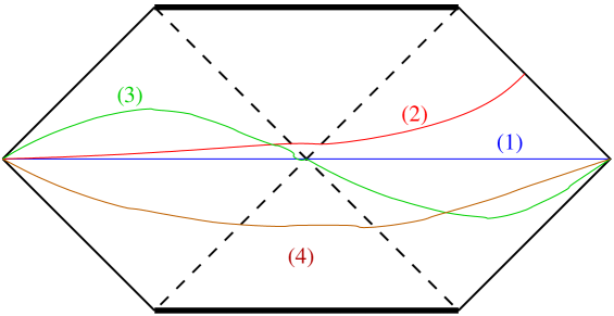
Figure 1: Schematic description of types of hypersurfaces covered by our main theorem: (1) a time symmetric Cauchy hypersurface, (2) a hyperboloid which also reaches one of the two spatial infinities, (3) a boosted slice, (4) a generic non-time symmetric Cauchy hypersurface.

Given a hypersurface $\mathcal{S}$ satisfying the conditions (5a) and (5b), the assumption of the existence of an asymptotically flat end with a non-vanishing ADM mass is sharp in order to be able to single out Schwarzschildean data. If, for example, no statement is made about the ADM momentum, then the initial data set can be either a Schwarzschildean one, or one corresponding to the C-metric. In this sense, our characterisation contains a global element. In order to obtain a purely local characterisation of Schwarzschild data, one would have to undertake, for example, a 3+1 decomposition of the characterisation of the Schwarzschild spacetime in terms of concomitants of the Weyl tensor obtained by Ferrando & Sáez [18] —this will be presented elsewhere.

The article is structured as follows: in section 2, we discuss the property of the D’Alambertian of the Weyl tensor of some vacuum Petrov type D spacetimes which is the keystone of our characterisation —the Zakharov property. A relation of the Petrov type D spacetimes satisfying this property is given. In section 3 we consider the 3+1 decomposition of the Zakharov property. In section 4 a discussion of which vacuum static Petrov type D spacetimes admit asymptotically Euclidean slices is given. Section 5 is concerned with the ADM 4-momentum of boost-rotation symmetric spacetimes. Finally, in section 6 the main results of the previous sections —propositions 1, 2, 3, 4— are recalled and put in context to render our main result, theorem 1. The shortcomings of our characterisation are discussed briefly, and a generalisation of the characterisation, valid for hyperboloidal data is given —see theorem 3. There is, also, an appendix is which some notation issues are addressed.

2 A result on type D spacetimes

Let $R_{\mu\nu\lambda\rho}$ denote the Riemann tensor of the metric $g_{\mu\nu}$. Our point of departure is the following curious result to be found in the Exact Solutions book [36]:

Theorem 2 (Zakharov 1965, 1970, 1972).

Vacuum fields satisfying the equation

$$R_{\mu\nu\lambda\rho;\sigma}^{\phantom{\mu\nu\lambda\rho;\sigma}\sigma}=\alpha R_{\mu\nu\lambda\rho},$$ (9)

for a certain function $\alpha$ are either type N ($\alpha=0$) or type D ($\alpha\neq 0$).

The proof of this theorem follows immediately from $R_{\mu\nu}=0$ and the identity [41]

$$R_{\mu\nu\lambda\rho;\sigma}^{\phantom{\mu\nu\lambda\rho;\sigma}\sigma}=R^{\sigma}_{\phantom{\sigma}\tau\mu\nu}R^{\tau}_{\phantom{\tau}\sigma\lambda\rho}+2(R^{\sigma}_{\phantom{\sigma}\mu\rho\tau}R^{\tau}_{\phantom{\tau}\lambda\nu\sigma}-R^{\sigma}_{\phantom{\sigma}\nu\rho\tau}R^{\tau}_{\phantom{\tau}\lambda\mu\sigma}),$$ (10)

written down with respect to a principal tetrad —see [39, 40]. The theorem 2 stems from attempts due to A.L. Zel’manov —in the case $\alpha=0$— of obtaining a characterisation of spacetimes containing gravitational radiation.

A direct evaluation shows that the property (9) —which we shall call the Zakharov property— is satisfied by the Schwarzschild spacetime, but for example, not by the Kerr solution. As the vacuum Petrov type D spacetimes are all known thanks to the work of Kinnersley [23], it is not too taxing to perform a casuistic analysis to see which are the ones satisfying the property (9). Kinnersley’s analysis made use of the Newman-Penrose (NP) formalism [27] and divides naturally into two cases: those solutions for which the NP spin coefficient $\rho$ —the expansion— vanishes and those for which it does not. The case with $\rho\neq 0$ divides, in turn, into 9 subcases. The solutions in case I have, in general, a non-vanishing NUT parameter, $l$. If $l=0$, then one obtains the Ehlers-Kundt solutions A1, A2 and A3 —see [16]. These solutions are static, and save the solution A1 (Schwarzschild) they are not asymptotically flat in the sense that there are no constants $k\geq 2$, $\beta>1/2$ for which

$$g_{\mu\nu}-\eta_{\mu\nu}=\mathcal{O}_{k}(r^{-\beta}).$$ (11)

The latter definition of asymptotic flatness has been borrowed from [5, 6] and will turn out to be most convenient for our endeavours. The $\rho\neq 0$ case II.A to II.F contain the Kerr-NUT solution and also other (non-asymptotically flat) solutions describing spinning bodies. The cases $\rho\neq 0$ III.A and III.B correspond, respectively, to the C-metric and its generalisation, the spinning C-metric. These solutions are known to be compatible (for particular ranges of the parameters) with the notion of asymptotic flatness —see [3, 8, 32]. Finally, the solutions with $\rho=0$ divide, in turn, in two classes A and B. The class A corresponds to the Ehlers-Kundt solutions B1 to B3 and are not asymptotically flat in the sense given by equation (11). The solutions of class A are spinning generalisations of class B. A summary of which of the vacuum Petrov type D spacetimes satisfy the Zakharov property, equation (9), is given in table 1. From there, we derive the following

Proposition 1.

The only type D solutions satisfying the Zakharov property, equation (9), are those with hypersurface orthogonal Killing vectors —that is, the Ehlers-Kundt solutions A1, A2, A3, B1, B2, B3 and C.

$\rho\neq 0$	case I (NUT metrics including Schwarzschild)	only if $l=0$
	case II.A (Kerr-NUT)	no
	case II.B	no
	case II.C	no
	case II.D	no
	case II.E	no
	case II.F	no
	case III.A (C-metric)	yes
	case III.B (twisting C-metric)	no
$\rho=0$	case A	yes
	case B	no

Table 1: Relation of the vacuum, type D spacetimes satisfying the Zakharov property. The description of the different cases follows the discussion given in Kinnersley’s analysis —see [23] and also [30]. The case I with $l=0$ corresponds to Ehlers-Kundt solutions A1 (Schwarzschild), A2 and A3. The case A corresponds to the Ehlers-Kundt solutions B1, B2 and B3 [16].

Arguably, of the spacetimes in table 1 satisfying the property (9) those of most interest are the Schwarzschild spacetime and the C-metric. For the Schwarzschild spacetime in the standard coordinates $(t,r,\theta,\varphi)$ the line element assumes the form

$$g_{S}=\left(1-\frac{2m}{r}\right)dt^{2}-\left(1-\frac{2m}{r}\right)^{-1}dr^{2}-r^{2}(d\theta^{2}+\sin^{2}\theta d\varphi^{2}),$$ (12)

nd the proportionality function is given by

$$\alpha_{S}=-\frac{6m}{r^{3}}.$$ (13)

On the other hand, for the C-metric in the coordinates $(t,x,y,p)$ —see e.g. [24]— such that

$$g_{C}=\frac{1}{A^{2}(x+y)^{2}}\left(F(y)dt^{2}-\frac{dx^{2}}{G(x)}-\frac{dy^{2}}{F(y)}-G(x)dp^{2}\right),$$ (14)

where

$$G(x)=1-x^{2}-2mAx^{3},\qquad F(y)=-1+y^{2}-2mAy^{3},$$ (15)

one has that

$$\alpha_{C}=-6A^{3}m(x+y)^{3}.$$ (16)

3 A $3+1$ decomposition

The property (9) in theorem 2 provides the cornerstone for a characterisation of the Schwarzschild spacetime that projects neatly under a 3+1 decomposition. The crucial observation is that in vacuum, the tensor

$$Z_{\mu\nu\lambda\rho}=R_{\mu\nu\lambda\rho;\sigma}^{\phantom{\mu\nu\lambda\rho;\sigma}\sigma}=C_{\mu\nu\lambda\rho;\sigma}^{\phantom{\mu\nu\lambda\rho;\sigma}\sigma},$$ (17)

where $C_{\mu\nu\lambda\rho}$ is the Weyl tensor of $g_{\mu\nu}$, is Weyl-like —that is, it is tracefree; $Z_{\mu\nu\lambda\rho}=Z_{\lambda\rho\mu\nu}=-Z_{\nu\mu\lambda\rho}=-Z_{\mu\nu\rho\lambda}$; and satisfies the first Bianchi identity $Z_{\mu\nu\lambda\rho}+Z_{\lambda\mu\nu\rho}+Z_{\nu\lambda\mu\rho}=0$.

Let $n^{\mu}$ be an unit timelike vector, and let us denote by $h^{\mu}_{\phantom{\mu}\nu}=g^{\mu}_{\phantom{\mu}\nu}-n^{\mu}n_{\nu}=\delta^{\mu}_{\phantom{\mu}\nu}-n^{\mu}n_{\nu}$ the associated projector. Following the notation and conventions of [20], we decompose the Weyl tensor as

$$C_{\mu\nu\lambda\rho}=2\bigg{(}l_{\mu[\lambda}E_{\rho]\nu}-l_{\nu[\lambda}E_{\rho]\mu}-n_{[\lambda}B_{\rho]\tau}\epsilon^{\tau}_{\phantom{\tau}\mu\nu}-n_{[\mu}B_{\nu]\tau}\epsilon^{\tau}_{\phantom{\tau}\lambda\rho}\bigg{)},$$ (18)

where

$$E_{\tau\sigma}=C_{\mu\nu\lambda\rho}h^{\mu}_{\phantom{\mu}\tau}n^{\nu}h^{\lambda}_{\phantom{\lambda}\sigma}n^{\rho},\quad B_{\tau\sigma}=C^{*}_{\mu\nu\lambda\rho}h^{\mu}_{\phantom{\mu}\tau}n^{\nu}h^{\lambda}_{\phantom{\lambda}\sigma}n^{\rho},$$ (19)

denote, respectively, the n-electric and n-magnetic parts of $C_{\mu\nu\lambda\rho}$, $\epsilon_{\tau\lambda\rho}=\epsilon_{\sigma\tau^{\prime}\lambda^{\prime}\rho^{\prime}}n^{\sigma}h^{\tau^{\prime}}_{\phantom{\tau^{\prime}}\tau}h^{\lambda^{\prime}}_{\phantom{\lambda^{\prime}}\lambda}h^{\rho^{\prime}}_{\phantom{\rho^{\prime}}\rho}$ is the spatial Levi-Civita tensor, $l_{\mu\nu}=h_{\mu\nu}+n_{\mu}n_{\nu}$, and $C^{*}_{\mu\nu\lambda\rho}=\frac{1}{2}C_{\mu\nu\tau\sigma}\epsilon^{\tau\sigma}_{\phantom{\tau\sigma}\lambda\rho}$ denotes the dual of $C_{\mu\nu\lambda\rho}$. The electric and magnetic parts of $C_{\mu\nu\lambda\rho}$ are symmetric, $E_{\mu\nu}=E_{\nu\mu}$, $B_{\mu\nu}=B_{\nu\mu}$, and traceless $E^{\mu}_{\phantom{\mu}\mu}=B^{\mu}_{\phantom{\mu}\mu}=0$. Moreover, they are spatial tensors in the sense that $E_{\mu\nu^{\prime}}h^{\nu^{\prime}}_{\phantom{\nu^{\prime}}\nu}=B_{\mu\nu^{\prime}}h^{\nu^{\prime}}_{\phantom{\nu^{\prime}}\nu}=0$; and $C_{\mu\nu\lambda\rho}=0$ if and only if $E_{\mu\nu}=B_{\mu\nu}=0$.

Using the embedding $\phi$, we can calculate the pull-backs of the electric and magnetic parts of $C_{\mu\nu\lambda\rho}$ to the hypersurface $\mathcal{S}$. Consequently, let us write $E_{ij}=(\phi^{*}E)_{ij}$ and $B_{ij}=(\phi^{*}B)_{ij}$. It is a direct consequence of the Codazzi equations that one can write

$$E_{ij}=r_{ij}+KK_{ij}-K_{ik}K^{k}_{\phantom{k}j},$$ (20a)

$$B_{ij}=-2\epsilon_{i}^{\phantom{i}kl}D_{k}K_{lj},$$ (20b)

where $r_{ij}$ denotes the Ricci tensor of the 3-metric $h_{ij}=(\phi^{*}h)_{ij}$. Thus, on $\mathcal{S}$, the electric and magnetic parts of the Weyl tensor can be entirely written in terms of the initial data $(h_{ij},K_{ij})$. Note, that in particular, for time symmetric spacetimes one has $B_{ij}=0$ as $K_{ij}=0$.

The tensor $Z_{\mu\nu\lambda\rho}$, being Weyl-like, admits a similar decomposition in terms of $n$-electric and $n$-magnetic parts, which we shall denote by $D_{\mu\nu}$ and $H_{\mu\nu}$, respectively. Hence, we write

$$Z_{\mu\nu\lambda\rho}=2\bigg{(}l_{\mu[\lambda}D_{\rho]\nu}-l_{\nu[\lambda}D_{\rho]\mu}-n_{[\lambda}H_{\rho]\tau}\epsilon^{\tau}_{\phantom{\tau}\mu\nu}-n_{[\mu}H_{\nu]\tau}\epsilon^{\tau}_{\phantom{\tau}\lambda\rho}\bigg{)},$$ (21)

where

$$D_{\tau\sigma}=Z_{\mu\nu\lambda\rho}h^{\mu}_{\phantom{\mu}\tau}n^{\nu}h^{\lambda}_{\phantom{\lambda}\sigma}n^{\rho},\quad H_{\tau\sigma}=Z^{*}_{\mu\nu\lambda\rho}h^{\mu}_{\phantom{\mu}\tau}n^{\nu}h^{\lambda}_{\phantom{\lambda}\sigma}n^{\rho},$$ (22)

and $Z^{*}_{\mu\nu\lambda\rho}=\frac{1}{2}Z_{\mu\nu\tau\sigma}\epsilon^{\tau\sigma}_{\phantom{\tau\sigma}\lambda\rho}$. As in the case of $E_{\mu\nu}$ and $B_{\mu\nu}$, one has that $D_{\mu\nu}=D_{\nu\mu}$, $H_{\mu\nu}=H_{\nu\mu}$, $D^{\mu}_{\phantom{\mu}\mu}=H^{\mu}_{\phantom{\mu}\mu}=0$, $D_{\mu\nu^{\prime}}h^{\nu^{\prime}}_{\phantom{\nu^{\prime}}\nu}=H_{\mu\nu^{\prime}}h^{\nu^{\prime}}_{\phantom{\nu^{\prime}}\nu}=0$; and $Z_{\mu\nu\lambda\rho}=0$ if and only if $D_{\mu\nu}=H_{\mu\nu}=0$.

For vacuum spacetimes, the identity (10) allows to write the tensors $D_{\mu\nu}$ and $H_{\mu\nu}$ as quadratic expressions of $E_{\mu\nu}$ and $B_{\mu\nu}$. A lengthy, but straightforward calculation renders the remarkably simple expressions:

$$D_{\mu\nu}=6\left(E_{\mu\sigma}E^{\sigma}_{\phantom{\sigma}\nu}-\frac{1}{3}h_{\mu\nu}E^{\sigma\tau}E_{\sigma\tau}\right)-6\left(B_{\mu\sigma}B^{\sigma}_{\phantom{\sigma}\nu}-\frac{1}{3}h_{\mu\nu}B^{\sigma\tau}B_{\sigma\tau}\right),$$ (23a)

$$H_{\mu\nu}=12\left(E_{\phantom{\sigma}(\mu}^{\sigma}B_{\nu)\sigma}-\frac{1}{3}h_{\mu\nu}E_{\sigma\tau}B^{\sigma\tau}\right).$$ (23b)

These expressions can be pulled-back to the hypersurface $\mathcal{S}$ by means of the embedding $\phi$ to obtain the following

Proposition 2.

Necessary conditions for an initial data set $(\mathcal{S},h_{ij},K_{ij})$ to be a Schwarzschildean initial data set are:

$$D_{ij}=\alpha E_{ij},$$ (24a)

$$H_{ij}=\alpha B_{ij},$$ (24b)

where $\alpha=-6m/r^{3}$, where $r$ is the standard Schwarzschild radial coordinate.

Note that the C-metric satisfies an analogous theorem with $\alpha=-6Am(x+y)^{3}$.

4 Asymptotic flatness and static type D spacetimes

In order to be able to discern Schwarzschildean data from among all those vacuum type D initial data sets satisfying the conditions $D_{ij}=\alpha E_{ij}$ and $H_{ij}=\alpha B_{ij}$, we require a couple of further results. Our first task is to get rid of those spacetimes which admit no slices with asymptotically Euclidean ends. Intuitively, it seems clear that a static spacetime which is not asymptotically flat should not admit slices with asymptotically flat ends. More precisely, one has the following

Proposition 3.

If a vacuum static spacetime is not asymptotically flat in the sense given by equation (11) —i.e. it belongs to the Ehlers-Kundt classes A2, A3 or B1, B2, B3— then it admits no slices with asymptotically Euclidean ends for which the decay conditions (4) hold.

It can be readily checked by direct computation that the spacetimes of the Ehlers-Kundt classes A2, A3 or B1, B2, B3 are not asymptotically flat in the sense discussed in the introduction. The proof of the proposition is by contradiction. Assume that our non-asymptotically flat, static spacetime, $\mathcal{M}$, admits a slice, $\mathcal{S}$, with an asymptotically Euclidean end for which the asymptotic decay conditions (4) hold. By construction, in this slice one has that $h_{ij}-\delta_{ij}=\mathcal{O}_{k}(r^{-\beta})$ and $K_{ij}=\mathcal{O}_{k-1}(r^{-1-\beta})$ with $\beta>1/2$ and $k\geq 2$. For this type of initial data the solution to the boost problem —see [11]— ensures the existence of a boost-type domain $\Omega_{r_{0},\theta}$ of the form

$$\Omega_{r_{0},\theta}=\big{\{}(t,x^{i})\in\mbox{\SYM R}\times\mbox{\SYM R}^{3}\;\big{|}\;|x|\geq r_{0},\;|t|\leq\theta|x|\big{\}},$$ (25)

for some constants $r_{0}$ and $\theta$, such that $r_{0}>0$ and $0<\theta<1$. From the fact that $\mathcal{M}$ is static, it follows that the slice $\mathcal{S}$ possesses a static Killing initial data set (KID). That is, there exists a pair $(N,X^{\mu})$, where $N$ is a scalar field and $X^{\mu}$ is a spatial vector field ($X^{\mu}h_{\mu\nu}=0$) such that $\xi^{\mu}|_{\mathcal{S}}=Nn^{\mu}+X^{\mu}$, where $\xi^{\mu}$ denotes the static Killing vector of the spacetime $\mathcal{M}$, and $n^{\mu}$ is the normal to $\mathcal{S}$. In what follows, let $X^{i}$ denote the pull-back of $X^{\mu}$, i.e. $X^{i}=(\phi^{*}X)^{i}$. Now, it is natural to consider the evolution of the initial data set $(h_{ij},K_{ij})$ along the flow given by the static Killing vector $\xi^{\mu}$. Thus, in $\Omega_{r_{0},\theta}$ one has that the spacetime metric is given by

$$g=-N^{2}dt^{2}+h_{ij}(dx^{i}+X^{i})(dx^{j}+X^{j}).$$ (26)

Recall that along this flow one has that $\partial_{t}h_{ij}=0$. Furthermore —see theorem 2.1 in [6] and also theorem 2.1 in [5]— the lapse $N$ and shift $X^{i}$ behave asymptotically as

$$N=1+\mathcal{O}_{k}(r^{-\beta}),$$ (27a)

$$X^{i}=\mathcal{O}_{k}(r^{-\beta}),$$ (27b)

with $\beta>1/2$ and $k\geq 2$. Thus, it follows that in $\Omega_{r_{0},\theta}$

$$g_{\mu\nu}-\eta_{\mu\nu}=\mathcal{O}_{k}(r^{-\beta}).$$ (28)

This is a contradiction to the assumption that spacetime is not asymptotically flat.

5 The ADM mass of the C-metric

The proposition 3 reduces our task of characterising Schwarzschildean initial data to finding a way of distinguishing between initial data corresponding to the C-metric and those corresponding to the Schwarzschild spacetime.

The C-metric belongs to the so-called boost-rotation symmetric spacetimes —see [10, 9, 32]—, that is, it possesses two commuting, hypersurface orthogonal Killing vectors. One of them is axial, and the other is of boost type. An argument outlined by Dray in [15] leads to

Proposition 4 (Dray, 1982).

The ADM 4-momentum of a boost-rotation symmetric spacetimes which is asymptotically flat —in the sense of equation (11)— vanishes.

Our strategy will be to make use of the latter result to discern between initial data sets corresponding to the C-metric, and those of the Schwarzschild spacetime.

Dray’s original argument lacks of some technical details, which we now proceed to fill. Let $(\mathcal{M},g)$ denote a boost-rotation symmetric spacetime, and let us denote by $\chi^{\mu}$, $\xi^{\mu}$, respectively the axial and boost Killing vectors of the spacetime. The vectors $\chi^{\mu}$ and $\xi^{\mu}$ commute. From the general theory of boost-rotation symmetric spacetimes given in [9] we know that there is a region of the spacetime —the one below the so-called roof— where the spacetime is static. The portion of the spacetime below the roof admits a boost-type domain, $\Omega_{r_{0},\theta}$, like the one in (25). From the fact that static spacetimes —and, in general, flat stationary spacetimes— admit a smooth null infinity —see e.g. [13]— and from the analysis of [6] it follows that on $\Omega_{r_{0},\theta}$ there exist matrices $\sigma_{\mu\nu}=\sigma_{[\mu\nu]}$, $\rho_{\mu\nu}=\rho_{[\mu\nu]}$ such that

$$\chi^{\mu}-\sigma^{\mu}_{\phantom{\mu}\nu}x^{\nu}=\mathcal{O}_{k}(r^{-\beta}),$$ (29a)

$$\xi^{\mu}-\rho^{\mu}_{\phantom{\mu}\nu}x^{\nu}=\mathcal{O}_{k}(r^{-\beta}),$$ (29b)

for $k\geq 2$ and $\alpha>1/2$, with $\sigma^{\mu}_{\phantom{\mu}\nu}\equiv\eta^{\mu\lambda}\sigma_{\lambda\nu}$, $\rho^{\mu}_{\phantom{\mu}\nu}\equiv\eta^{\mu\lambda}\rho_{\lambda\nu}$, and $\eta_{\mu\nu}$ denoting the Minkowski metric. Without loss of generality assume that the axis of symmetry of the axial Killing vector lies along the $x^{3}$ axis. Accordingly,

$$\sigma_{\mu\nu}x^{\nu}=(0,-x^{2},x^{1},0),$$ (30a)

$$\rho_{\mu\nu}x^{\nu}=(-x^{3},0,0,-t).$$ (30b)

Thus, from the commuting nature of the two Killing vectors $\chi^{\mu}$ and $\xi^{\mu}$ it follows that

$$\sigma^{\mu}_{\phantom{\mu}\nu}=\begin{pmatrix}0&0&0&0\\ 0&0&-1&0\\ 0&1&0&0\\ 0&0&0&0\end{pmatrix},\quad\rho^{\mu}_{\phantom{\mu}\nu}=\begin{pmatrix}0&0&0&-1\\ 0&0&0&0\\ 0&0&0&0\\ -1&0&0&0\end{pmatrix}.$$ (31)

One can associate to the boost-type domain $\Omega_{r_{0},\theta}$, provided that $k\geq 2$ and $\beta>1/2$, in an unique way an ADM 4-momentum vector $p^{\mu}$ —see e.g. [4, 12]. It follows from the theory developed in [6] that

$$\sigma^{\mu}_{\phantom{\mu}\nu}p^{\nu}=\rho^{\mu}_{\phantom{\mu}\nu}p^{\nu}=0,$$ (32)

whence necessarily

$$p^{\mu}=0,$$ (33)

which is the observation made by Dray in [15]. As a side remark, note that the above result needs not to hold if the Killing vectors are non-commuting.

6 Concluding remarks

Our main theorem —see the introductory section— follows directly from the propositions 1, 2, 3 and 4.

It is clear from the argumentation that the conditions to single out the Schwarzschild solution are sharp. In particular, as seen from proposition 4 if no remark on the ADM 4-momentum is made, initial data for the C-metric is included. Precisely because of this condition, it is that our argumentation can not be extended to include hyperboloidal initial data sets not intersecting spatial infinity like the ones discussed in [35]. Intuitively, in the case of hyperboloidal data one would try to replace the condition on the ADM 4-momentum by some condition regarding the Bondi 4-momentum. However, it is well known that the Bondi mass of boost-rotation symmetric spacetimes is non-vanishing —see e.g. [32]. An alternative is to replace the condition on the ADM 4-momentum by a condition on the so-called Newman-Penrose (NP) constants [28, 29]. The NP constants vanish for the Schwarzschild spacetime —see e.g. [14]—, but are non-vanishing for the C-metric —cfr. e.g. [26]. Friedrich & Kánnár [21] have shown how these quantities defined at null infinity can be expressed in terms of Cauchy initial data. In principle, the NP constants are also expressible in terms of hyperboloidal data —the details of this have not yet been worked out, and will be pursued elsewhere. Accordingly, we state —without going fully into the details— the following

Theorem 3.

Let $\mathcal{S}$ be a 3-manifold with a hyperboloidal end, and let $(h_{ij},K_{ij})$ be a pair of symmetric tensors on $\mathcal{S}$ satisfying the Einstein vacuum constraints. If there is a function $\alpha$ such that the conditions (5a) and (5b) hold, i.e.

$$D_{ij}=\alpha E_{ij},\quad H_{ij}=\alpha B_{ij},$$ (34)

then the triplet $(\mathcal{S},h_{ij},K_{ij})$ corresponds to a slice of the Schwarzschild spacetime.

For a discussion on the appropriate boundary conditions giving rise to a hyperboloidal end, the reader is remitted to [19] —see also [1] and reference therein.

The question whether the theorems 1 or 2 can be used to construct Schwarzschildean initial data sets with especial properties —for example boosted slices with vanishing mean curvature, if these exist— remains open. In any case, the conditions (5a) and (5b) are necessary conditions for an initial data set to be Schwarzschildean. Also, it would be of interest to see if it is possible to obtain a reformulation of (5a) and (5b) which does not contain the function $\alpha$. These ideas will be pursued elsewhere.

Appendix A The notation $\mathcal{O}_{k}$

In this article we follow the $\mathcal{O}_{k}$ notation introduced in [6]. Given a function $\phi$ on the boost-type domain $\Omega_{r_{0},\theta}$, we say that $\phi=\mathcal{O}_{k}(r^{\beta})$, for $\beta\in\mbox{\SYM R}$, if $\phi\in C^{k}(\Omega_{r_{0},\theta})$ and there is a function $C(t)$ such that

$$|\partial_{\alpha_{1}}\cdots\partial_{\alpha_{i}}\phi|\leq C(t)(1+|x|)^{\beta-i},\quad 0\leq i\leq k.$$

References

- [1] L. Andersson & P. T. Chruściel, Hyperboloidal Cauchy data for vacuum Einstein equations and obstructions to smoothness of null infinity, Phys. Rev. Lett. 70, 2829 (1993).
- [2] R. Arnowitt, S. Deser, & C. W. Misner, The dynamics of General Relativity, in Gravitation: an introduction to current research, edited by L. Witten, page 227, John Wiley & Witten, 1962.
- [3] A. Ashtekar & T. Dray, On the existence of solutions to Einstein’s field equations with non-zero Bondi news, Comm. Math. Phys. 79, 581 (1981).
- [4] R. Bartnik, The mass of an asymptotically flat manifold, Comm. Pure Appl. Math. , 661 (1986).
- [5] R. Beig & P. T. Chruściel, Killing vectors in asymptotically flat spacetimes. I. Asymptotically translational Killing vectors and rigid positive energy theorem, J. Math. Phys. 37, 1939 (1996).
- [6] R. Beig & P. T. Chruściel, The isometry group of asymptotically flat, asymptotically empty spacetimes with timelike ADM four-momentum, Comm. Math. Phys. 188, 585 (1997).
- [7] R. Beig & N. O’Murchadha, Late time behaviour of the maximal slicing of the Schwarzschild black hole, Phys. Rev. D 57, 4728 (1998).
- [8] J. Bičák & V. Pravda, Spinning C-metric: radiative spacetime with accelerating, rotating black holes, Phys. Rev. D 60, 044004 (1999).
- [9] J. Bičák & B. G. Schmidt, Asymptotically flat radiative space-times with boost-rotation symmetry: the general structure, Phys. Rev. D 40, 1827 (1989).
- [10] W. B. Bonnor, The sources of the vacuum C-metric, Gen. Rel. Grav. 15, 535 (1983).
- [11] D. Christodoulou & N. O’Murchadha, The boost problem in general relativity, Comm. Math. Phys. 80, 271 (1981).
- [12] P. T. Chruściel, Boundary conditions at spatial infinity from a Hamiltonian point of view, in Topological properties and global structure of space-time, edited by P. Bergmann & V. de Sabbata, page 49, Plenum Press, 1986.
- [13] S. Dain, Initial data for stationary spacetimes near spacelike infinity, Class. Quantum Grav. 18, 4329 (2001).
- [14] S. Dain & J. A. Valiente Kroon, Conserved quantities in a black hole collision., Class. Quantum Grav. 19, 811 (2002).
- [15] T. Dray, On the asymptotic flatness of the C metrics at spatial infinity, Gen. Rel. Grav. 14, 109 (1982).
- [16] J. Ehlers & W. Kundt, Exact solutions of the gravitational field equations, in Gravitation: an introduction to current research, edited by L. Witten, Wiley, 1962.
- [17] F. Estabrook, H. Wahlquist, S. Christensen, B. DeWitt, L. Smarr & E. Tsiang, Maximally slicing a black hole, Phys. Rev. D 7, 2814 (1973).
- [18] J. J. Ferrando & J. A. Sáez, An intrinsic characterization of the Schwarzschild metric, Class. Quantum Grav. 15, 1323 (1998).
- [19] H. Friedrich, Cauchy problems for the conformal vacuum field equations in General Relativity, Comm. Math. Phys. 91, 445 (1983).
- [20] H. Friedrich, Hyperbolic reductions for Einstein’s equations, Class. Quantum Grav. 13, 1451 (1996).
- [21] H. Friedrich & J. Kánnár, Bondi-type systems near space-like infinity and the calculation of the NP-constants, J. Math. Phys. 41, 2195 (2000).
- [22] A. Karlhede, On a coordinate-invariant description of Riemannian manifolds, Gen. Rel. Grav. 12, 963 (1980).
- [23] W. Kinnersley, Type D vacuum metrics, J. Math. Phys. 10, 1195 (1969).
- [24] W. Kinnersley & M. Walker, Uniformly accelerating charged mass in general relativity, Phys. Rev. D 2, 1359 (1970).
- [25] M. D. Kruskal, Maximal extension of Schwarzschild metric, Phys. Rev. D 119, 1743 (1960).
- [26] R. Lazkoz & J. A. Valiente-Kroon, Boost-rotation symmetric type D radiative metrics in Bondi coordinates, Phys. Rev. D 62, 084033 (2000).
- [27] E. T. Newman & R. Penrose, An approach to gravitational radiation by a method of spin coefficients, J. Math. Phys. 3, 566 (1962).
- [28] E. T. Newman & R. Penrose, 10 exact gravitationally-conserved quantities, Phys. Rev. Lett. 15, 231 (1965).
- [29] E. T. Newman & R. Penrose, New conservation laws for zero rest-mass fields in asymptotically flat space-time, Proc. Roy. Soc. Lond. A 305, 175 (1968).
- [30] E. T. Newman, L. Tamburino & T. Unti, Empty-space generalization of the Schwarzschild metric, J. Math. Phys. 4, 915 (1963).
- [31] N. O’Murchadha & K. Roszkowski, Embedding spherical spacelike slices in a Schwarzschild solution, in gr-qc/0307050.
- [32] V. Pravda & A. Pravdová, Boost-rotation symmetric spacetimes —review, Czech. J. Phys. 50, 333 (2000).
- [33] B. L. Reinhart, Maximal foliations of extended Schwarzschild space, J. Math. Phys. 14, 719 (1973).
- [34] M. A. Scheel, T. W. Baumgarte, G. B. Cook, S. L. Shapiro & S. A. Teukolsky, Treating instabilities in a hyperbolic formulation of Einstein’s equations, Phys. Rev. D 58, 044020 (1998).
- [35] B. G. Schmidt, Data for the numerical calculation of the Kruskal space-time, in The Conformal structure of space-time. Geometry, Analysis, Numerics, edited by J. Frauendiener & H. Friedrich, Springer, 2002.
- [36] H. Stephani, D. Kramer, M. A. H. MacCallum, C. Hoenselaers & E. Herlt, Exact Solutions of Einstein’s Field Equations, Cambridge University Press, 2003, Second edition.
- [37] J. A. Valiente Kroon, Asymptotic expansions of the Cotton-York tensor on slices of stationary spacetimes, Class. Quantum Grav. 21, 3237 (2004).
- [38] J. W. York Jr, Energy and momentum of the gravitational field, in Essays in General Relativity, edited by F. J. Tipler, page 39, New York, 1980, Academic Press.
- [39] V. D. Zakharov, A physical characteristic of Einstenian spaces of degenerate type II in the classification of Petrov (in Russian), Dokl. Akad. Nauk. SSSR 161, 563 (1965).
- [40] V. D. Zakharov, Algebraical and group theoretical methods in general relativity: Invariant Petrov type characterisation of the type of Einstein spaces (in Russian), Prob. Teor. Grav. Elem. Chastitis 3, 128 (1970).
- [41] V. D. Zakharov, Gravitational waves in Einstein’s theory of gravitation, Nauka, Moscow, 1972.