Local conditions for the generalized covariant entropy bound

Abstract

A set of sufficient conditions for the generalized covariant entropy bound given by Strominger and Thompson is as follows: Suppose that the entropy of matter can be described by an entropy current $s^{a}$. Let $k^{a}$ be any null vector along $L$ and $s\equiv-k^{a}s_{a}$. Then the generalized bound can be derived from the following conditions: (i) $s^{\prime}\leq 2\pi T_{ab}k^{a}k^{b}$, where $s^{\prime}=k^{a}\nabla_{a}s$ and $T_{ab}$ is the stress energy tensor; (ii) on the initial 2-surface $B$, $s(0)\leq-\frac{1}{4}\theta(0)$, where $\theta$ is the expansion of $k^{a}$. We prove that condition (ii) alone can be used to divide a spacetime into two regions: The generalized entropy bound holds for all light sheets residing in the region where $s<-\frac{1}{4}\theta$ and fails for those in the region where $s>-\frac{1}{4}\theta$. We check the validity of these conditions in FRW flat universe and a scalar field spacetime. Some apparent violations of the entropy bounds in the two spacetimes are discussed. These holographic bounds are important in the formulation of the holographic principle.

I Introduction

Bounds on entropy set by some specified area that surrounds a certain volume are called holographic bounds and are important in the formulation of the holographic principle of ’t Hooft. There are several such bounds, the one that concerns us here is a generalization of the covariant entropy bound. The covariant entropy bound, conjectured by Bousso, is the following bousso ; bn ; three : Let $B$ be a spacelike 2-surface in a spacetime $(M,g_{ab})$ satisfying Einstein’s equation and the dominant energy condition. Its area is denoted by $A_{B}$. Consider a null hypersurface $L$ generated by null geodesics, each with tangent vector field $k^{a}$ which starts at $B$ and is orthogonal to $B$. Suppose that the expansion

$$\theta=\nabla_{a}k^{a}$$ (1)

of $k^{a}$ is non-positive everywhere on $L$ and $L$ is not terminated until a caustic is reached (where $\theta\rightarrow-\infty$). Then the entropy, $S_{L}$, through $L$ satisfies

$$S_{L}\leq\frac{1}{4}\,A_{B}\,.$$ (2)

Evidences supporting this bound have been studied in situations where other non-covariant bounds fail, such as in cosmological spacetimes and other matter systems bousso ; bn ; three ; viqar ; gaolemos . The null surface $L$ in the conjecture is required to be extended as far as possible unless a caustic is reached. Flanagan et. al  three modify this bound by allowing $L$ to be terminated at some spacelike 2-surface $B^{\prime}$ before coming to a caustic. Then the inequality (2) is replaced by

$$S_{L}\leq\frac{1}{4}\,(A_{B}-A_{B^{\prime}}).$$ (3)

This is called the generalized covariant entropy bound, or the generalized Bousso bound.

Recently, Strominger and Thompson quan suggested a set of simple assumptions from which the generalized bound (3) can be derived. The authors in quan assumed that the matter entropy can be described in terms of an entropy current $s^{a}$, where $s^{a}$ is independent of the null surface $L$. Apart from this, the following two conditions are postulated: (i) Let

$$s\equiv-k^{a}s_{a}\,$$ (4)

be the flux of entropy that crosses the light sheet $L$. Let

$$s^{\prime}=k^{a}\nabla_{a}s\,$$ (5)

be the rate of entropy flux on $L$ and $T_{ab}$ be the stress-energy tensor. Then

$$s^{\prime}\leq 2\pi T_{ab}k^{a}k^{b}\,,$$ (6)

i.e., the rate of entropy flux is less than the energy flux throughout the light sheet.

(ii) On the initial 2-surface $B$, where the affine parameter $\lambda$ is set to zero,

$$s(0)\leq-\frac{1}{4}\,\theta(0).$$ (7)

Only local quantities are involved in conditions (i) and (ii). Bousso, et. al simple suggested a similar set of sufficient conditions which is stronger, and we do not discuss it here.

Conditions (6) and (7) apply to spacetimes where absolute entropy currents (i.e., entropy currents that do not depend on the light sheet) are well defined. Moreover, as we shall show explicitly in Proposition 1, condition (i) becomes superfluous for testing the generalized bound, when condition (ii) is regarded as a pointwise condition, in which case it gives a straightforward criteria for the generalized covariant bound. Thus, we suggest an even simpler assumption from which the generalized entropy bound can be derived: (A) Given a spacetime region one has

$$s(x)\leq-\frac{1}{4}\,\theta(x)\,,$$ (8)

where $x$ represents any spacetime point within the region.

This is just a generalization of Thomson and Strominger’s condition (ii), from an initial surface, to the whole region. Armed with this condition we can prove Proposition 1 (see next section for the precise formulation and proof), which states that a necessary and sufficient condition for the generalized entropy bound to be satisfied for all light sheets in a region, is that condition (A) (i.e., $s\leq-\frac{1}{4}\theta$) is satisfied. Then, the bound holds in the region where $s<-\frac{1}{4}\theta$ and fails in the region where $s>-\frac{1}{4}\theta$. There are, however, some violations. Indeed, since $\theta\simeq 0$ for light sheets in a small neighborhood of the apparent horizon, this result indicates that if the apparent horizon is located in a matter system (where $s=s_{\rm matter}>0$) the generalized covariant entropy bound is generally violated for light-sheets in a sufficiently small neighborhood of the apparent horizon. In such a neighborhood one surely has $s>-\frac{1}{4}\theta$. However, as we will see along the paper, such kind of violation is due to a collapse of the hydrodynamic description of matter entropy for light sheets in a small neighborhood of the apparent horizon. We therefore treat this kind of violations as trivial violations (see also Bousso et. al simple ).

We shall apply Proposition 1 to two cases, namely, to a closed Friedmann-Robertson-Walker (FRW) universe and to a scalar field spacetime. In both cases absolute entropy currents $s^{a}$ can be defined.

In the first case, a FRW universe, we test condition (A) and show that it is valid throughout the spacetime except for regions very close to the singularity and the apparent horizon. Thus, following the previous discussion, we conclude that there is no meaningful violation to the generalized covariant entropy bound in the cosmological spacetime. Then from Proposition 1 we know that the generalized covariant entropy bound holds. For completeness we also test Thomson and Strominger conditions (i) and (ii) (although (ii) is automatically satisfied when (A) is satisfied) and show they hold. In this manner we complete the analysis made in bousso for some selected light sheets in a FRW universe.

In the second case, a time dependent spherically symmetric massless scalar field spacetime, the issue is more interesting, since it yields a new example for testing the bounds. This spacetime is characterized by a past spacelike singularity, a timelike naked singularity and an apparent horizon. Such a study has been initiated by Husain viqar where covariant entropy bounds in such a time dependent spherically symmetric massless scalar field spacetime were examined. We reexamine this issue by checking the sufficient condition (A) (see Equation (8)) and make improvements in the following aspects: First, we find that the formula of the entropy density proposed in viqar is valid only in a region that does not include the neighborhood of the naked timelike singularity. Second, Husain viqar identified, in an unusual energy-temperature relation, the coefficient $\sigma$ with the Stefan-Boltzmann constant. However, $\sigma$ remains undetermined and the value $\sigma=\frac{1}{2}$ adopted in viqar is by no means generic. Using $\sigma=\frac{1}{2}$, Husain found no violation for the original Bousso bound (2). On the other hand we find that in some regions of this spacetime the bound is violated. We check the Bousso bound for light sheets hitting the past spacelike singularity and find that the Bousso bound is violated for such light sheets starting near the apparent horizon. This violation can not be explained by the failure of the fluid description for short light sheets, but can be rescued by a smaller value of $\sigma$. Thus, by using the covariant entropy bound one can put an upper limit in $\sigma$. Third, Husain viqar found that the generalized bound is violated for light sheets in the neighborhood of the apparent horizon. This can be easily explained by our Proposition 1, since as we have argued, near the apparent horizon $\theta\simeq 0$, and it is trivial to have matter satisfying $s>-\frac{1}{4}\theta$ in violation of the bound. By calculating $s(x)$ and $\theta(x)$ we can find the boundary hypersurface $s=-\frac{1}{4}\theta$. According to Proposition 1 the bound is violated in the region in-between the apparent horizon and this boundary. Fourth and final, a length scale argument simple has been used to eliminate counterexamples for the generalized bound. This argument states that if the proper distance of the path traveled by the light sheet is smaller than the thermal wavelength of the matter then the hydrodynamic description for the matter fails. Now, Husain viqar showed that for some light sheets the bound is violated and this violation cannot be explained by the length scale argument. Thus, in these cases, the argument is inconclusive to eliminate counterexamples for the generalized bound. In our analysis, we reach a similar conclusion. However, the length scale used in viqar is a black body length scale, $\rho^{-1/4}$, which is not consistent with our analysis of the scalar field, where we show one should use an associated length scale of the form $\rho^{-1/6}$.

In this paper, we use units with $c=k_{B}=\hbar=G=1$ and the $(-,+,+,+)$ metric signature.

II Proposition

In this section, we propose a simple but useful criteria for the generalized covariant entropy bound.

Proposition 1

A necessary and sufficient condition for the generalized entropy bound to be satisfied for all light sheets in a region is that condition (A), i.e., $s\leq-\frac{1}{4}\,\theta$, is satisfied everywhere in the region.

Proof: We use the coordinate system $(\lambda,x^{1},x^{2})$ introduced in three to describe the light sheet $L$, where $(x^{1},x^{2})$ is any coordinate system on the initial two-surface $B$ and $\lambda$ is the affine parameter of the the null generators. Associated with each generator, one can define an area-decreasing factor three :

$${\cal A}(\lambda)\equiv\exp\left[\int_{0}^{\lambda}d\bar{\lambda}\theta(\bar{\lambda})\right],$$ (9)

which has the following obvious properties:

$${\cal A}(0)=1,$$ (10)

and

$${\cal A}^{\prime}(\lambda)={\cal A}(\lambda)\theta(\lambda).$$ (11)

Then the entropy crossing $L$ can be expressed as three

$$S_{L}=\int_{B}d^{2}x\,\sqrt{\det h_{AB}(x)}\int_{0}^{\lambda_{\infty}(x)}d\lambda\,s(x,\lambda)\,{\cal A}(x,\lambda),$$ (12)

where $x\equiv(x^{1},x^{2})$ is a point on $B$, $h_{AB}(x)$ is the induced 2-metric on $B$, $\lambda_{\infty}(x)$ is the affine parameter at the endpoint of the generator which starts at $x$ on $B$ and ends on $B^{\prime}$, $s(x,\lambda)$ is the entropy density at the point $(x_{1},x_{2},\lambda)$, and ${\cal A}(x,\lambda)$ is the area-decreasing factor for the null generator that starts at point $x$. Following three , we shall rescale the affine parameter along each generator such that $\lambda_{\infty}(x)=1$ at $B^{\prime}$. Then, from Eqs. (11) and (12), if $s\leq-\frac{1}{4}\,\theta$ in the neighborhood of the light sheet, we have

$$S_{L} \leq -\frac{1}{4}\int_{B}d^{2}x\sqrt{\det h_{AB}(x)}\int_{0}^{1}d\lambda\,{\cal A}^{\prime}(x,\lambda)$$ (13)

$$= \frac{1}{4}\int_{B}d^{2}x\sqrt{\det h_{AB}(x)}\,[{\cal A}(x,0)-{\cal A}(x,1)]$$

$$= \frac{1}{4}\,(A_{B}-A_{B}^{\prime}).$$

In the last step, we have used the formulas given in three :

$$A_{B} = \int_{B}d^{2}x\sqrt{\det h_{AB}(x)}\,,$$ (14)

$$A_{B^{\prime}} = \int_{B}d^{2}x\sqrt{\det h_{AB}(x)}{\cal A}(x,1)\,.$$ (15)

Note that the result in Eq. (13) is independent of the rescaling for $\lambda_{\infty}(x)$. Thus, we have proved the sufficient part.

Now we prove the necessary part of the proposition. If the inequality (13) holds for all light sheets in a region, choose any one of them, and for convenience do a different rescaling of the affine parameter, such that $\lambda_{\infty}(x)=\Delta\lambda$. Let $B$ shrink to a sufficiently small area and let $B^{\prime}$ be sufficiently close to $B$ (i.e., $\Delta\lambda\rightarrow 0$). Then we obtain the “local version” of Eq. (12)

$$S_{L}=s(0)\,A_{B}\,\Delta\lambda,$$ (16)

where $s(0)$ is the entropy density on $B$ (since $B$ has shrunk to an arbitrarily small area, $s$ can be treated as a constant on $B$) and we have used Eqs. (10) and (14). On the other hand, Eq. (15) becomes

$$A_{B^{\prime}} = \int_{B}d^{2}x\sqrt{\det h_{AB}(x)}{\cal A}(\Delta\lambda)$$ (17)

$$= A_{B}[{\cal A}(0)+{\cal A}^{\prime}(0)\Delta\lambda].$$

Hence,

$$A_{B}-A_{B^{\prime}}=-A_{B}\,{\cal A}^{\prime}(0)\,\Delta\lambda.$$ (18)

Substituting Eq. (16) and Eq. (18) into Eq. (3) we get condition (A), which is what we wanted to show.

By investigating condition (A), we shall be able to identify the regions where the bound holds for all the light sheets lying inside it. It is worth noticing that Proposition 1 does not cover the case when a light sheet crosses both the $s>-\frac{1}{4}\,\theta$ zone and the $s<-\frac{1}{4}\,\theta$ zone.

Our next remark explores the implication of Strominger and Thompson’s sufficient conditions (i) and (ii).

Remark   Suppose conditions (i) and (ii) in quan are satisfied for a light sheet $L$. Then $s\leq-\frac{1}{4}\,\theta$ is satisfied at all points on $L$.

The proof of this remark was almost given in quan . Under the two conditions, it is shown in quan that

$$s(\lambda)\leq-\frac{1}{2}\frac{G^{\prime}(\lambda)}{G(\lambda)},$$ (19)

where $G\equiv\sqrt{{\cal A}}$. It then follows immediately, from Eq. (11), that $s\leq-\frac{1}{4}\,\theta$ all over the light sheet.

Proposition 1 and the Remark imply that the role of condition (i) could almost be replaced by the single condition (A). If condition (A) is satisfied everywhere on the light sheet, then Proposition 1 guarantees that the generalized Bousso bound is satisfied, no matter whether condition (i) is violated or not. On the other hand, if condition (A) holds on the initial surface $B$ but not throughout the light sheet, the Remark means that condition (i) must fail at some points on the light sheet. So verifying condition (i) will not help judge the generalized Bousso bound. In section III.2.2, we show that there exist light sheets which satisfy the generalized Bousso bound, but condition (i) fails everywhere on the light sheets. Therefore, condition (i) is not a necessary condition for the bound. Further implications of these conditions will be discussed in the applications of the following section.

III Applications

III.1 Application to a closed universe

We consider a closed, dust-dominated FRW universe which is described by the metric

$$ds^{2}=a^{2}(\eta)(-d\eta^{2}+d\chi^{2}+\sin^{2}\chi d\theta^{2}+\sin^{2}\chi\sin^{2}\theta d\varphi^{2})\,,$$

(20)

where

$$a(\eta)=\frac{a_{\rm max}}{2}(1-\cos\eta)\,.$$ (21)

In order to test our condition (A) and condition (i) of Thompson and Strominger quan we need some preliminaries. The Planck proper time, $\tau_{PL}$ (where $\tau_{PL}\sim 1$), corresponds to the coordinate time $\eta=\eta_{PL}$, which is obtained from Eqs. (20) and (21) as $\eta_{PL}\sim a_{\rm max}^{-1/3}$ bousso . Now we choose the future-directed outgoing light sheet such that its tangent vector is given by

$$k^{a}=(\partial/\partial\eta)^{a}+(\partial/\partial\chi)^{a}.$$ (22)

Since such a universe is homogeneous and evolves adiabatically, the physical entropy density ${s}_{\rm phys}$ takes the form earlyuni

$${s}_{\rm phys}(\eta)=\frac{s_{0}}{a^{3}(\eta)},$$ (23)

where $s_{0}$ is a constant. $s_{0}$ can be specified by the requirement that the entropy density may not exceed one at the Plank time. Since, with the help of Eq. (21), $a^{3}(\eta_{PL})\sim a_{\rm max}$, we have $s_{0}\sim a_{\rm max}$. Note also that the four-velocity of a comoving observer is

$$u^{a}=\frac{1}{a(\eta)}\left(\frac{\partial}{\partial\eta}\right)^{a}\,.$$ (24)

Thus, the entropy flux can be constructed as

$$s^{a}={s}_{\rm phys}(\eta)\,u^{a}=\frac{s_{0}}{a^{4}(\eta)}\left(\frac{\partial}{\partial\eta}\right)^{a}.$$ (25)

Then the entropy associated with $k^{a}$ is

$$s(\eta)=-s_{a}k^{a}=\frac{4}{a_{\rm max}(1-\cos(\eta))^{2}}.$$ (26)

To test condition (A), we calculate the expansion of $k^{a}$,

$$\theta=2\left(\cot(\eta/2)+\cot\chi\right).$$ (27)

It is easy to see that testing condition (A) is equivalent to testing the following inequality

$$\left|\frac{4s}{\theta}\right|=\left|\frac{\csc^{3}\eta\,\csc(\eta/2+\chi)\,\sin\chi}{a_{\rm max}}\right|\leq 1.$$ (28)

In Plank units, $a_{\rm max}$ is a very large number. Then very close to the singularity, $\eta<\eta_{PL}$, one has that the expression inside the absolute value in Eq. (28) goes as $|\eta_{PL}^{3}/\eta^{3}|$, and so the inequality Eq. (28) fails in that region. This is not a real violation of the bound because the region is inside the quantum regime. In addition, the inequality may fail around $\chi=\pi-\eta/2$, where $\theta=0$. Now, this is where the apparent horizon is located. Thus, as long as a light sheet does not go sufficiently close to the apparent horizon (by definition, a light sheet can never cross the apparent horizon), the generalized entropy bound always holds. As discussed in the introduction, light sheets that are located in a small neighborhood of the apparent horizon should not be of our concern since the hydrodynamic description fails there. We conclude that the generalized entropy bound always holds if light sheets are reasonably chosen (not too close to the singularities or to the apparent horizon).

Now we test condition (i) of Thompson and Strominger quan . The derivative of the entropy flux, $s^{\prime}$, in condition (i) for the FRW universe (see Eq. (20)) is given by

$$s^{\prime}(\eta)=k^{a}\nabla_{a}s=-\frac{8\sin\eta}{a_{\rm max}(1-\cos\eta)^{3}}.$$ (29)

It is also straightforward to compute the energy flux through the light sheet,

$$T_{ab}k^{a}k^{b}=\frac{3}{4\pi(1-\cos\eta)}.$$ (30)

Since $T_{ab}k^{a}k^{b}$ is positive, to test condition (i), it is sufficient to test the following inequality

$$\frac{|s^{\prime}(\eta)|}{2\pi T_{ab}k^{a}k^{b}}=\frac{16|\sin\eta|}{3a_{\rm max}(1-\cos\eta)^{2}}\leq 1.$$ (31)

In Plank units, $a_{\rm max}$ is a very large number. So inequality (31) can be violated only when $\eta$ is sufficiently small (or by symmetry, sufficiently close to $2\pi$). The detail can be seen by power series expansion of $\frac{|s^{\prime}(\eta)|}{2\pi T_{ab}k^{a}k^{b}}$ around $\eta=0$. The leading term is

$$\frac{|s^{\prime}(\eta)|}{2\pi T_{ab}k^{a}k^{b}}\sim\frac{64}{3a_{\rm max}\eta^{3}}.$$ (32)

Therefore, only when $\eta\lesssim 2.77\,a_{\rm max}^{-1/3}=2.77\eta_{PL}$, can inequality (31) be violated. However, this violation takes place within a few Plank times from the singularity, where quantum gravity takes effect. Thus, the violation does not occur in the classical regime. Condition (ii) of Thompson and Strominger quan is a particular instance of our condition (A) and therefore has been tested above.

III.2 Application to a scalar field spacetime

III.2.1 The exact scalar field solution

We shall now review the scalar field solution presented in viqar ; ss . From the Einstein-scalar field equations for massless minimally coupled scalars, a spherically symmetric solution is given by the metric

$$ds^{2} = -t\,f(r)\,dt^{2}+t\,f(r)^{-1}\,dr^{2}$$ (33)

$$+t\,r^{2}\,f(r)^{-\frac{1+\sqrt{3}/2}{\sqrt{3}/2}}\left(d\theta^{2}+\sin^{2}\theta d\phi^{2}\right),$$

where

$$f(r)=\left(1-\frac{2}{r}\right)^{-\frac{\sqrt{3}}{2}}\,.$$ (34)

(There is also a possibility of choosing $-\frac{\sqrt{3}}{2}$ where there is $\frac{\sqrt{3}}{2}$ in Eqs. (33) and (34) but we do not consider it here). The corresponding scalar field in the spacetime is

$$\phi(t,r)=\frac{1}{4\sqrt{\pi}}\ln\left[t^{\sqrt{3}}\,f(r)^{1/\sqrt{3}}\right].$$ (35)

For future discussions, we introduce the following properties of the spacetime. The future directed tangent vector field of the radial ingoing null geodesics is

$$k^{a}=\frac{1}{f(r)\,t}\left(\frac{\partial}{\partial t}\right)^{a}-\frac{1}{t}\left(\frac{\partial}{\partial r}\right)^{a}\,.$$ (36)

The corresponding expansion is

$$\theta=\frac{1}{t}-\frac{1}{t_{\rm AH}(r)},$$ (37)

where

$$t_{\rm AH}(r)=\frac{r^{2}}{2\left(r-1+\sqrt{3}/2\right)}\,f(r)^{-1-\frac{2}{\sqrt{3}}},$$ (38)

and the equation $t=t_{\rm AH}(r)$ yields the apparent horizon as a function of $r$.

In order to proceed our investigation in a perfect fluid context, we need to define comoving observers. As suggested in viqar , one may choose the four-velocity of the observers to be parallel to $\partial^{a}\phi$. This requires that $\partial^{a}\phi$ be timelike. Using Eq. (33) one finds

$$\partial_{a}\phi=\sqrt{\frac{3}{\pi}}\,\frac{1}{4t}\,dt_{a}+\frac{f^{\prime}(r)}{4\sqrt{3\pi}f(r)}\,dr_{a}\,.$$ (39)

Then a straightforward calculation shows that $(\partial\phi)^{2}\equiv\partial_{a}\phi\,\partial^{a}\phi$, given by

$$(\partial\phi)^{2}=g^{ab}\partial_{a}\phi\partial_{b}\phi$$ (40)

$$= \frac{1}{48\pi t^{3}}\left(\frac{r-2}{r}\right)^{\sqrt{3}/2}\left(-9+\frac{3\left(\frac{r-2}{r}\right)^{-\sqrt{3}}t^{2}}{(r-2)^{2}r^{2}}\right)$$ (41)

is negative only for

$$t<G(r)\equiv\sqrt{3}(r-2)^{1+\sqrt{3}/2}r^{1-\sqrt{3}/2}\,.$$ (42)

Thus, our discussion should be confined to the region $t<G(r)$, where $\partial^{a}\phi$ is timelike and comoving observers can exist. As mentioned in viqar , the spacetime has two curvature singularities located at $t=0$ and $r=2$. Fig. 1 shows the plots of the two singularities, the apparent horizon, and $t=G(r)$.

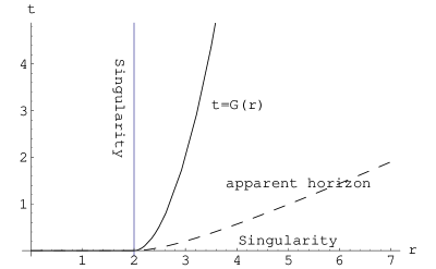
Figure 1: A spacetime diagram for the scalar field spacetime. Below the solid line $t=G(r)$, $\partial^{a}\phi$ is timelike. Between $t=G(r)$ and the timelike singularity $r=2$, no observers associated with the scalar field can be naturally defined.

Now we review the derivation of the entropy flux 4-vector in the framework of viqar . Assume the scalar field is a perfect fluid with stress-energy tensor

$$T_{ab}=\rho u_{a}u_{b}+P(u_{a}u_{b}+g_{ab}).$$ (43)

On the other hand, the stress-energy tensor can be calculated from the metric (33) as

$$T_{ab}=\partial_{a}\phi\,\partial_{b}\phi-\frac{1}{2}g_{ab}(\partial\phi)^{2}\,.$$ (44)

Define

$$u^{a}=-\frac{\partial^{a}\phi}{\sqrt{-(\partial\phi)^{2}}}$$ (45)

and rewrite Eq. (44) as

$$T_{ab}=-\frac{1}{2}(\partial\phi)^{2}u_{a}u_{b}-\frac{1}{2}(\partial\phi)^{2}(u_{a}u_{b}+g_{ab}).$$ (46)

When $\partial^{a}\phi$ is timelike, $u^{a}$ may be identified as the 4-velocity of observers comoving with the scalar field. Therefore, by comparing Eq. (43) and Eq. (46), we have the following relation

$$P=\rho=-\frac{1}{2}(\partial\phi)^{2}.$$ (47)

Now define

$$\omega=k\,,$$ (48)

where $k$ is the amplitude of the scalar field wave vector ${\bf k}$. The energy-momentum dispersion relation is assumed of the form viqar :

$$\epsilon=\gamma\,\omega^{\beta}$$ (49)

where $\gamma$ and $\beta$ are constants to be determined. We now calculate the relevant thermodynamic quantities for the scalar field. It is well-known that the mean occupation number $\overline{n_{k}}$ for a Bose gas is (see e.g. landau )

$$\overline{n_{k}}=\frac{1}{e^{(\epsilon_{k}-\mu)/T}-1}\,$$ (50)

where, $\epsilon_{k}$ is the energy in mode $k$, $\mu$ is the chemical potential, $T$ is the temperature of the gas, and we set the Boltzmann constant $k_{\rm B}=1$. Note that $\mu=0$ for the scalar field. Following a canonical ensemble standard calculation, we find that the free energy $F$ inside a volume $V$ is

$$F = \frac{TV}{2\pi^{2}}\int_{0}^{\infty}\omega^{2}\log(1-e^{-\gamma\omega^{\beta}/T})d\omega$$ (51)

$$= -\frac{V\,T^{(3+\beta)/\beta}}{2\pi^{2}\,\beta\,\gamma^{3/\beta}}\,\Gamma\left(\frac{3}{\beta}\right)\,\zeta\left(1+\frac{3}{\beta}\right)\,.$$

Other thermodynamic quantities can be easily derived from the free energy $F$. First, we find the relations

$$P = \frac{\beta}{3}\,\rho$$ (52)

$$\rho = \frac{1}{36\,\gamma}\,T^{2}\,.$$ (53)

From Eqs. (52) and (47), the constant $\beta$ can be identified immediately as

$$\beta=3\,.$$ (54)

Here, the constant $\gamma$ remains undetermined. Eq. (53) is a Stefan-Boltzmann law for a gas in one spatial dimension. In viqar , the coefficient of $T^{2}$ was indeed identified with a Stefan-Boltzmann constant $\sigma$, $\sigma=1/36\gamma$.

The entropy density, ${s}_{\rm phys}$, takes the form

$${s}_{\rm phys}=2\sigma T\,.$$ (55)

Combining Eqs. (45) , (47), (53) and (55), we obtain the entropy flux 4-vector:

$$s^{a}={s}_{\rm phys}\,u^{a}=-\sqrt{2\sigma}\,\partial^{a}\phi\,.$$ (56)

Husain viqar chose $\sigma=\frac{1}{2}$ such that

$$s^{a}=-\partial^{a}\phi.$$ (57)

In order to compare our results with that in viqar , we shall follow this choice and use Eq. (57) to compute entropy.

III.2.2 Testing entropy bounds for future-directed ingoing light sheets

We shall study the light sheets which are generated by the future-directed ingoing null vectors $k^{a}$ given in Eq. (36). From Eqs. (35), (36) and (57), we have the entropy density associated with the null vector:

$$s=-s_{a}k^{a}=\frac{1}{4\sqrt{\pi}t^{2}}\left[\sqrt{3}\left(\frac{r-2}{r}\right)^{\frac{\sqrt{3}}{2}}+\frac{t}{r^{2}-2r}\right]\,.$$ (58)

It is also straightforward to calculate $s^{\prime}$ and $T_{ab}k^{a}k^{b}$.

Figure 2: A spacetime diagram depicting the important regions under discussion. Condition (i) is satisfied below the thick solid line, while condition (A) is valid above the thin solid line. The dotted line represents the apparent horizon.

In Fig. 2 we show explicitly where these conditions are satisfied. We see that there exists a region where condition (A) is valid but condition (i) fails. If a light sheet lies in this region, then the covariant bound is satisfied, although condition (i) fails everywhere on the light sheet. This illustrates that condition (i) in quan is not a necessary condition for the entropy bound.

An important point to note is that the Proposition 1 does not cover the case when a light sheet crosses the $s=-\frac{1}{4}\theta$ line. In Fig. 3(a), a light sheet starts near the apparent horizon and crosses the $s=-\frac{1}{4}\theta$ line. This standard light sheet has an initial 2-sphere with fixed radius $r_{0}$ and fixed area $A_{0}$. We can truncate this standard light sheet at any other inner radius $r$ to get a truncated light sheet with a given initial 2-sphere specified by $r_{0}$ and $A_{0}$. By proceeding inwards with this truncation we get a series of light sheets, each labeled by the coordinate $r$ and area $A(r)$ at which it is truncated, all starting at the same initial 2-sphere ($r_{0}$,$A_{0}$). We shall test the bound for each one of them. Define

$${\rm ratio}(r)=\frac{1}{4}\frac{S(r)}{A_{0}-A(r)},$$ (59)

where $S(r)$ is the entropy passing through the light sheet starting from the fixed 2-sphere with area $A_{0}$ and ending at the 2-sphere with area $A(r)$. If ${\rm ratio}(r)\leq 1$, the generalized bound, Eq. (3), is satisfied. Fig. 3(b) plots the change of ${\rm ratio}\,(r)$. The $\rm ratio$ is larger than unity in the $s>-\frac{1}{4}\theta$ zone, and it remains larger than unity after the light sheet enters the $s<-\frac{1}{4}\theta$ zone until about $r=140$.

In order to decide whether this means a solid violation of the generalized Bousso bound, we first check in which scale the fluid description of the matter fails. The entropy flux computation is invalid if the light sheet is shorter than the matter thermal wavelength viqar ; simple . The thermal wavelength $\lambda$ is estimated from the relation $\lambda\sim 1/k$, where $k$ is the momentum of a fluid particle. From Eq. (48) and the energy-momentum dispersion relation Eq. (49) ($\beta=3$), we have

$$\lambda\sim\frac{1}{\bar{\epsilon}^{1/3}}$$ (60)

where $\bar{\epsilon}$ is the mean energy per particle. To estimate $\bar{\epsilon}$, we first calculate the particle number density, $n$, by integrating the occupation number $\overline{n_{k}}$ (see Eq. (50)) over all modes:

$$n = \frac{1}{\pi^{2}}\int_{0}^{\infty}\overline{n_{k}}\omega^{2}d\omega$$ (61)

$$= \frac{1}{\pi^{2}}\int_{0}^{\infty}\frac{1}{e^{\omega^{3}/T}-1}\omega^{2}d\omega$$

$$\sim T$$

Noting that the energy density $\rho\sim T^{2}$ (see Eq. (53)), we have immediately $\bar{\epsilon}=\rho/n\sim T$. Therefore, Eq. (60) gives the thermal wavelength $\lambda\sim T^{-1/3}$. From Eq. (53), we finally obtain

$$\lambda\sim\rho^{-1/6}\,.$$ (62)

(This is different from the length scale $\rho^{-1/4}$ given in viqar , which follows a black body radiation calculation, but we believe is not a consistent estimation for the scalar field.)

Figure 3: (a) A light sheet crossing the $s=-\frac{1}{4}\theta$ surface. AH represents the apparent horizon. (b) Change of ratio on the light sheet. The generalized bound is violated in the $s>-\frac{1}{4}\theta$ zone and is satisfied until the light sheet runs certain distance in the $s<-\frac{1}{4}\theta$ zone.

Figure 4: Plots of the proper length and thermal wavelength $\lambda$ for the light sheet in Fig. 3(a). This figure shows that the proper length of the light sheet is significantly larger than the thermal wavelength $\lambda$.

Now, after this preamble, we consider the light sheet as in Fig. 3(a). We let it start near the apparent horizon and stop at $r=140$ where the $\rm ratio$ is close to but larger than $1$ according to Fig. 3(b). We define the proper length of the light sheet as the length between two comoving observers, one that passes the starting point (near the apparent horizon) and the other that passes the ending point of the light sheet (near $r=140$). Since the comoving frame is not static, this proper length, $L$, changes with time and can be easily calculated from the metric (33) as:

$$L(t)=\int_{r_{0}}^{r_{f}}\sqrt{\frac{t}{f(r)}},$$ (63)

where $r_{0}$ and $r_{f}$ are the radial coordinates of the two comoving observers. Along the light sheet, $t$ is a function of $r$, so the proper length, $L$, can be expressed as a function of $r$, as plotted in Fig. 4. The thermal wavelength $\lambda$ is a function of the temperature. The temperature at each point on the light-sheet is a function of $r$, so $\lambda$ is a function of $r$. This is also plotted in Fig. 4. Since $\lambda$ is always much smaller than the proper length, the local entropy description is justified for the light sheet. Thus the generalized Bousso bound is not valid in this case.

III.2.3 Testing the entropy bounds for past-directed ingoing and past-directed outgoing light sheets

We first investigate the generalized Bousso bound for the light sheets generated by past-directed ingoing null geodesics. The tangent field of these null geodesics takes the form:

$$k^{a}=-\frac{1}{f(r)\,t}\left(\frac{\partial}{\partial t}\right)^{a}-\frac{1}{t}\left(\frac{\partial}{\partial r}\right)^{a}\,.$$ (64)

The entropy density is $s=s_{a}k^{a}$ (note that the sign of this expression is different from that in Eq. (58) for $k^{a}$ in Eq. (64) is past-directed), and the expansion for $k^{a}$ can be calculated straightforwardly. To check condition (A), we consider the following expression

$$s+\frac{1}{4}\theta = \frac{1}{4(r-2)t^{2}}\left[\left(-1+\sqrt{\frac{3}{\pi}}\right)\left(\frac{r-2}{r}\right)^{1+\frac{\sqrt{3}}{2}}r\right.$$ (65)

$$+ \left.\left(2-2r-\sqrt{3}-\frac{1}{\sqrt{\pi}}\right)\frac{t}{r}\right]\,.$$

Since $r>2$, we see immediately that $s+\frac{1}{4}\theta<0$ in the whole spacetime, i.e., condition (A) is satisfied everywhere. Thus, according to Proposition 1, the generalized Bousso bound holds for all past-directed ingoing light sheets. Consequently, the original Bousso bound holds for all these light sheets. Therefore, with the help of Proposition 1, both the covariant entropy bounds for past-directed ingoing light sheets have been easily tested.

Now we investigate the generalized Bousso bound for the light sheets generated by past-directed outgoing null geodesics. This is much more complicated. The tangent field of these null geodesics is

$$k^{a}=-\frac{1}{f(r)\,t}\left(\frac{\partial}{\partial t}\right)^{a}+\frac{1}{t}\left(\frac{\partial}{\partial r}\right)^{a}\,.$$ (66)

These light sheets must be located in the past of the apparent horizon and may terminate at the past singularity $t=0$. Fig. 5 shows that condition (A) is violated in a neighborhood of the apparent horizon. Indeed, it holds only near the spacelike singularity. An analysis similar to the one done in section III.2.2 shows that the generalized Bousso bound is violated for light sheets between the apparent horizon and the $s=-\frac{1}{4}\theta$ surface. One can also check that condition (i) is nowhere satisfied in the past of the apparent horizon.

The importance and interest of past-directed (both ingoing and outgoing) light sheets is that it enables us to investigate the original Bousso bound, since these light sheets can reach the past singularity. Consider then a specific light sheet which starts at the apparent horizon with coordinates $(t_{0},r_{0})=(13.25,30)$ and terminates at the past singularity with coordinates $(t_{f},r_{f})=(0,43.9)$, see Fig. 6(a). The $\rm ratio$ for this light sheet is ratio$=1.545$, indicating that the covariant entropy bound is violated, apriori. One can fix the ending 2-sphere at the singularity and move continuously the initial 2-sphere along the original light sheet, labeling each initial 2-sphere by its coordinate $r$, and test the Bousso bound for all these light sheets. This is done in Fig. 6(b), where we obtain the $\rm ratio(r)$ as a function of the initial 2-sphere $r$. We see that the maximum violation occurs when the light sheet starts at the apparent horizon, the case shown in Fig. 6(a).

Figure 5: A spacetime diagram showing the region where condition (A) $s<-\frac{1}{4}\theta$ holds for past-directed outgoing light sheets.

Figure 6: (a) A past-outgoing light sheet located between the apparent horizon and the past singularity. (b) Plot of $\rm ratio(r)$ when the light sheet in part (a) of this figure rolls down from the apparent horizon to the singularity.

Figure 7: Plots of the proper length and thermal wavelength $\lambda$ for the light sheet in Fig. 6(a). We consider the light sheet as in Fig. 6(a), but we let it start near the apparent horizon and stop it at $r=43.9$ where the singularity is located. Since the comoving frame is not static, this proper length changes with time. But along the light sheet, the time $t$ is a function of $r$. So the proper length can be plotted as a function of $r$. This figures shows that the proper length of the light sheet is significantly larger than the thermal wavelength $\lambda$.

Similarly to the discussion in section III.2.2, we shall compare the proper length of the light sheet with the matter thermal wavelength. As plotted in Fig. 7, the proper length between the two observers passing the light sheet changes with $r$. As well the matter thermal wavelength changes with $r$. We see that the proper length of the light sheet dominates $\lambda$ all the way. Therefore, the length scale argument does not save the covariant entropy bound.

We still have a trump on the sleeve, which is the Stefan-Boltzmann constant $\sigma$. Remember we have followed Husain’s choice $\sigma=1/2$ viqar , but this does not need to be the case. Since the entropy for any light sheet is proportional to $\sqrt{\sigma}$ (see Eq. (56)), the bound could be rescued by choosing a smaller value of $\sigma$. In Table 1 we give the $\rm ratio$ for four light sheets that start at the apparent horizon with coordinates $(t_{0},r_{0})$, and end at the spacelike singularity with coordinates $(t,r)=(0,r_{f})$, where $r=r_{f}$ is the radial coordinate of the light sheets at the singularity. It shows that the $\rm ratio$ for these (and by inference all) light sheets starting at the apparent horizon and ending at the singularity is almost a constant. The reason behind this coincidence is unknown to us, but this fact is very instructive for fixing the covariant bound. We can also let the initial 2-sphere of each light sheet in Table 1 move away from the apparent horizon and plot the change of $\rm ratio(r)$ as a function of the initial 2-sphere labeled by $r$. It turns out that their behaviors are all similar to that in Fig. 6(b). Therefore, if the entropy density (56) is scaled down by a factor smaller than $1/1.547$, the bound will be saved. This corresponds to requiring $\sigma\leq 0.21$. Thus the covariant Bousso bound puts an upper limit on the constant $\sigma$.

Table 1:   The coordinates for the starting spherical surfaces at the apparent horizon are $(t_{0},r_{0})$. Thus, all light sheets begin at the apparent horizon and end at the spacelike singularity $(t,r)=(0,r_{f})$, where $r=r_{f}$ is the radial coordinate of the light sheets at the singularity.

$t_{0}$	$r_{0}$	$r_{f}$	$\rm ratio$
$13.25$	$30$	$43.9$	$1.545$
$1498$	$3000$	$4498$	$1.546$
$5998$	$12000$	$17998$	$1.547$
$59998$	$120000$	$179998$	$1.547$

IV Conclusions

We have investigated the sufficient conditions for the generalized covariant entropy bound proposed by Strominger and Thompson quan . We showed that the condition $s(x)\leq-\frac{1}{4}\,\theta(x)$, our condition (A), can be used to identify the regions where the generalized entropy bound is satisfied for all light sheets. We applied this condition to a closed, dust-dominated FRW universe and a scalar field spacetime. We have found that in the closed FRW spacetime, condition (A) is satisfied in most of the spacetime. Violations occur only in the regions very close to the apparent horizon and the singularity. According to our Proposition 1, the generalized Bousso bound is violated in these regions. But such violations are due to the breakdown of the local description of entropy and the breakdown of classical relativity. Then, following the original investigation by Husain, we have studied the covariant entropy bounds in a scalar field spacetime. Husain has found that the generalized covariant entropy bound is violated only in a band region around the apparent horizon surface. Proposition 1 indicates that such a band region exists in spacetimes where the matter entropy does not vanish in a neighborhood of the apparent horizon. We also have checked the validity of the local description of entropy for a light sheet which violates the generalized entropy bound. It turns out that the proper length of the light sheet is much larger than the thermal wavelength, meaning the entropy computation is valid in this case. Our formula for the thermal wavelength, $\lambda\sim\rho^{-1/6}$, is consistent with the dispersion relation of the scalar field. This is different from Husain’s estimation $\lambda\sim\rho^{-1/4}$, which obviously follows a black body argument. Husain showed that there is no violation for the covariant entropy bound by calculating the entropy of light sheets hitting the timelike singularity $r=2$. Our calculation shows that the comoving observers are no longer timelike near the timelike singularity. Consequently, there is no meaningful definition for entropy in that region. In contrast, we have considered the past-directed light sheets which hit the past singularity $t=0$. We have checked condition (A) for past-directed ingoing light sheets and found it holds for all of them. According to Proposition 1, both the generalized and the original Bousso bounds hold for such light sheets. For past-directed outgoing light sheets starting near the apparent horizon, violations of the bounds have been found. However, these violations rely on the artificially selected Stefan-Boltzmann constant $\sigma$. Our numerical results suggest that the covariant entropy bound can be rescued by choosing a smaller value of $\sigma$. Therefore, the entropy bound conjecture sets an upper bound on $\sigma$.

Acknowledgments

This work was partially funded by Fundação para a Ciência e Tecnologia (FCT) - Portugal through project POCTI/FNU/44648/2002. SG acknowledges financial support by the FCT grant SFRH/BPD/10078/2002 from FCT. JPSL thanks Observatório Nacional do Rio de Janeiro for hospitality.

References

- (1) R. Bousso, JHEP 9907 004 (1999).
- (2) R. Bousso, Rev. Mod. Phys. 74, 825 (2002).
- (3) E.E. Flanagan, D. Marolf and R. Wald, Phys. Rev. D 62, 084035 (2000).
- (4) V. Husain, Phys. Rev. D 69, 084002 (2004).
- (5) S. Gao and J. P. S. Lemos, JHEP 0404 017 (2004).
- (6) A. Strominger and D. Thompson, Phys. Rev. D 70, 044007 (2004).
- (7) R. Bousso, E. E. Flanagan and D. Marolf, Phys. Rev. D 68, 064001 (2003).
- (8) E. W. Kolb and M. S.Turner, The Early Universe, (Addison-Wesley, 1990).
- (9) V. Husain, E. Martinez and D. Nunez, Phys. Rev. D 50, 3783 (1994).
- (10) L. D. Landau and E. M. Lifshitz, Statistical Physics, 3rd edition, Butterworth-Heinemann, Oxford, 1980.