Black hole head-on collisions and gravitational waves with fixed mesh-refinement and dynamic singularity excision

Abstract

We present long-term-stable and convergent evolutions of head-on black hole collisions and extraction of gravitational waves generated during the merger and subsequent ring-down. The new ingredients in this work are the use of fixed mesh-refinement and dynamical singularity excision techniques. We are able to carry out head-on collisions with large initial separations and demonstrate that our excision infrastructure is capable of accommodating the motion of the individual black holes across the computational domain as well as their merger. We extract gravitational waves from these simulations using the Zerilli-Moncrief formalism and find the ring-down radiation to be, as expected, dominated by the $\ell=2$, $m=0$ quasi-normal mode. The total radiated energy is about $0.1\,\%$ of the total ADM mass of the system.

I Introduction

One of the most urgent problems currently under investigation in general relativity is the coalescence of binary compact objects. The importance of this scenario largely arises from its significance for the new research field of gravitational wave astronomy; ground-based gravitational wave interferometric detectors, such as LIGO, GEO600, VIRGO and TAMA, have started collecting data. The in-spiral and merger of neutron stars and black holes is considered among the most promising sources of gravitational radiation to be detected by these instruments. Theoretical predictions of the resulting wave patterns will be important both for the detection and for the physical interpretation of such measurements. Although approximation techniques have been remarkably successful, the theoretical calculation of wave forms from compact object binaries will most likely require the numerical solution of the Einstein field equations.

Very important milestones have been achieved recently in the numerical modeling of compact object binaries. For instance, a few orbits of binary neutron stars are now possible (see e.g. Shibata et al. (2003); Marronetti et al. (2004); Miller et al. (2004)). Also, with binary black holes, Brügmann et al. Brügmann et al. (2004) have been able to carry out evolutions lasting for timescales longer than one orbital period. These varied efforts in modeling compact binary systems with numerical relativity share a common goal – to extract accurate waveform templates (see Miller (2005) for a study on accuracy requirements of such waveform calculations). This “Holy Grail” of numerical relativity, however, still eludes the community. A unique problem faced in the simulation of black hole spacetimes is the presence of physical singularities, which makes this task particularly delicate from a numerical point of view.

For a long time after the pioneering work of Eppley and Smarr in the 1970s Eppley (1975); Smarr et al. (1976); Smarr (1979), progress in numerical black hole evolutions was rather slow, and the codes suffered from instabilities after relatively short times. In contrast, the last few years have seen a change of strategy in the area of numerical relativity. More emphasis has been put on analyzing the structure of the evolution equations underlying the numerical codes (see e.g. Shibata and Nakamura (1995); Friedrich (1996); Frittelli and Reula (1996); Anderson and York (1999); Baumgarte and Shapiro (1999); Alcubierre et al. (2000); Kidder et al. (2001); Yoneda and Shinkai (2002); Sarbach and Tiglio (2002); Bona et al. (2003)). In combination with increased computational resources and advanced treatments of the spacetime singularities, this has led to vastly improved stability properties in the evolution of spacetimes with a single black hole either at rest or moving through the computational domain Alcubierre and Brügmann (2001); Yo et al. (2002); Alcubierre et al. (2003a); Sperhake et al. (2004). In view of these encouraging results, attention has been shifting again toward the application of these techniques to the evolution and merger of binary black holes (see e.g. Brandt et al. (2000); Alcubierre et al. (2003a); Brügmann et al. (2004); Alcubierre et al. (2004a, b)).

In this paper, we will focus on the numerical evolution of head-on collisions of black holes implemented in the framework of dynamical singularity excision. The study of head-on colliding black holes has attracted a good deal of attention in the past, both numerically and analytically. We have already mentioned the early work of Eppley and Smarr who numerically evolved Misner data for equal-mass black hole collisions in axisymmetry. The waveforms extracted from these evolutions differ little in amplitude and phase from those obtained in perturbative calculations Smarr (1979). The head-on collision was re-investigated numerically in the 1990s Anninos et al. (1993); Anninos et al. (1995a, b); Baker et al. (1997); Anninos and Brandt (1998) with generally good agreement between numerical results and those obtained from perturbation theory for various initial configurations. As a whole, the approximate analytic study of binary black hole head-on collisions has been remarkably successful and has generated a wealth of literature. The late stage of the collision, when the separation of the two holes is sufficiently small, is well described by the close limit approximation (see e.g. Price and Pullin (1994); Abrahams and Cook (1994) as well as Gleiser et al. (1996) for an estimate of the quality of the approximation using second-order perturbation theory). Similarly the particle approximation has been used to describe the in-fall phase with large black-hole separation either in the framework of post-Newtonian theory (see e.g. Simone et al. (1995)) or using Newtonian trajectories with appropriate modifications Anninos et al. (1995a, b). In particular, Anninos et al. Anninos et al. (1995b) combined their “particle-membrane” technique with results from close limit calculations to provide estimates of the total radiated energy that are in good agreement with the results of numerical relativity over the whole range of initial black hole separations (see their Fig. 11).

The encouraging results of these perturbative approximations gave rise to the idea of combining them with full numerical evolutions via matching on slices of constant time. With this temporal matching, it was possible to extend the life of simulations of binary black holes which would otherwise stop because of numerical instabilities. This is now commonly known as the “Lazarus” approach; developed by Baker et al. Baker et al. (2000) it has demonstrated good waveform agreement with non-linear evolutions.

The general picture that has emerged in analytic as well as numerical studies of equal mass head-on collisions is that gravitational wave emission is dominated by the $\ell=2$, $m=0$ quasi-normal oscillations of the post-merger black hole and that the total radiated wave energy is typically less than a percent of the system’s ADM mass.

In spite of their limited astrophysical relevance, simulations of black hole head-on collisions still represent an important problem. In view of the eventual target, the in-spiral and merger of a binary black hole, these simulations constitute a key milestone in the development of numerical codes, a natural next step after successful evolutions of single black holes. While numerical codes have continued to improve in the simulation of head-on or grazing collisions Brügmann (1999); Brandt et al. (2000); Alcubierre et al. (2001a), long-term-stable simulations have only been obtained rather recently by Alcubierre et al. Alcubierre et al. (2003a) using the puncture method. In Alcubierre et al. (2004a) the combination of this approach with the “Simple Excision” technique of Alcubierre and Brügmann Alcubierre and Brügmann (2001) has been shown to preserve the long-term stability and yield good agreement in the wave forms. Almost parallel to this work black hole head-on collisions have been simulated in the framework of mesh refinement Fiske et al. (2005) and fourth-order finite differencing techniques Zlochower et al. (2005). In this paper we present the first such long-term-stable evolutions obtained in fixed mesh-refinement as well as using the dynamical singularity excision technique.

The simulations presented in this paper have been obtained with the Maya evolution code. This code and in particular its dynamical singularity excision technique are described in detail in Shoemaker et al. (2003) (referred to as Paper 1 from now on). A key development in recent months has been the combination of the Maya code with the mesh-refinement package Carpet Schnetter et al. (2004). Carpet has enabled us to push the outer boundaries substantially further out than was possible with the uni-grid version of Maya; this was crucial in the extraction of gravitational wave signals.

The paper is organized as follows: The construction of binary black hole initial data used in this work is described in Sec. II, while the details of the numerical evolution scheme are given in Sec. III. The gravitational waveforms are analyzed in Sec. IV with regard to their convergence properties and the physical information they provide. We conclude in Sec. V with a discussion of our results and the implications for future work. In the appendix we present the details of the wave extraction using the Zerilli-Moncrief formalism on a single black hole background in Kerr-Schild coordinates. Throughout the paper, units are given in terms of $M$, with $M=\,^{A}m+\,^{B}m$, the sum of the bare masses of the individual black holes in the binary.

II Initial data

The construction of astrophysically meaningful initial data for simulations of compact binaries is a highly non-trivial problem and represents an entire branch of research in numerical relativity (see Cook (2000) for a detailed overview).

For the simulations discussed in this work, we construct initial data according to the procedure of Matzner et al. Matzner et al. (1998), referred to from now on as “HuMaSh” data. This type of data has been used, for example, in binary grazing-collision evolutions by Brandt et al. Brandt et al. (2000). The starting point of the HuMaSh data is the Kerr-Schild spacetime metric

$$g_{\mu\nu}=\eta_{\mu\nu}+2\,H\,l_{\mu}\,l_{\nu}\,,$$ (1)

where $\eta_{\mu\nu}$ is the Minkowski metric, and $l_{\mu}$ is a null-vector with respect to both $g_{\mu\nu}$ and $\eta_{\mu\nu}$. In terms of 3+1 quantities, the Kerr-Schild metric is given by

$$\gamma_{ij} = \delta_{ij}+2\,H\,l_{i}\,l_{j}\,,$$ (2)

$$\alpha = (1+2\,H\,l^{t}\,l^{t})^{-1/2}\,,$$ (3)

$$\beta^{i} = -\frac{2\,H\,l^{t}\,l^{i}}{1+2\,H\,l^{t}\,l^{t}}\,.$$ (4)

In particular, for a non-rotating black hole of mass $m$ at rest at the origin

$$H = \frac{m}{r}\,,$$ (5)

$$l_{\mu} = (1,\vec{l})\,,$$ (6)

$$\vec{l} = \frac{\vec{x}}{r}\,,$$ (7)

with $r=\sqrt{\delta_{ij}\,x^{i}\,x^{j}}$.

As pointed out in Ref. Matzner et al. (1998), Kerr-Schild coordinates have two attractive features. First, with relevance to singularity excision, the coordinates penetrate the horizon. Second, the Kerr-Schild spacetime metric is form-invariant under a boost transformation. Specifically, under a boost $v$ along the $z$-axis, all that changes is

$$H = \frac{m}{R},$$

$$l_{\mu} = \left[\frac{\gamma\,(R-v\,Z)}{R},\frac{x}{R},\frac{y}{R},\frac{\gamma\,(Z-v\,R)}{R}\right],$$

where $\gamma=1/\sqrt{1-v^{2}}$, $Z\equiv\gamma(z-v\,t)$, and $R^{2}\equiv x^{2}+y^{2}+Z^{2}$.

A spatial metric approximating initial data of two black holes, with bare masses $\,{}^{A}m$ and $\,{}^{B}m$ respectively, can be given by

$$\gamma_{ij} = \,{}^{A}\gamma_{ij}+\,^{B}\gamma_{ij}-\delta_{ij}\,,$$ (8)

where the $\,{}^{A}\gamma_{ij}$ and $\,{}^{B}\gamma_{ij}$ are to be understood as the Kerr-Schild spatial metric (2) evaluated at the corresponding black hole coordinate position and boost velocity. Following the HuMaSh prescription, the extrinsic curvature is constructed from

$$K^{i}\,_{j} = \,{}^{A}K^{i}\,_{j}+\,^{B}K^{i}\,_{j}\,,$$ (9)

where the $\,{}^{A}K^{i}\,_{j}$ and $\,{}^{B}K^{i}\,_{j}$ are also to be understood as the Kerr-Schild extrinsic curvature evaluated at the corresponding black hole coordinate position and boost velocity.

It is important to point out that the HuMaSh data do not provide a close limit; that is, as the coordinate separation of the black holes shrinks to zero, the resulting metric is not that of a single black hole with mass $M={}^{A}m+{}^{B}m$. Furthermore, as given by (8) and (9), the HuMaSh data do not satisfy the Einstein constraints. As suggested by Marronetti et al. Marronetti et al. (2000), one could attenuate the constraint violations of the HuMaSh data using an exponential damping factor. Bonning et al. Bonning et al. (2003) used this attenuating procedure and provided a fairly detailed investigation of the general properties of the underlying HuMaSh data. In particular, they show that it has the correct gravitational binding energy in the Newtonian far-separation limit.

By construction the HuMaSh data will satisfy the constraint equations only in the limit of infinite separation of the two black holes. A rigorous treatment of a scenario with finite separation would thus require using the HuMaSh data as freely-specifiable background data and then solving the Hamiltonian and momentum constraint according to York’s initial data prescription York (1979). Since one of our primary goals is to extract gravitational waves from the black hole simulations, we need a sufficiently large computational domain, only attainable via mesh-refinement. Unfortunately, elliptic solvers operating on numerical grids with various refinement levels have not yet been developed in our Maya code. Using the uni-grid solvers available, on the other hand, is computationally prohibitive. Therefore, as with the grazing collision work in Ref. Brandt et al. (2000), the simulations in this paper were obtained using the constraint-violating HuMaSh initial data.

In this context one has to keep in mind that the constraints will always be violated at the level of numerical accuracy in a real simulation.

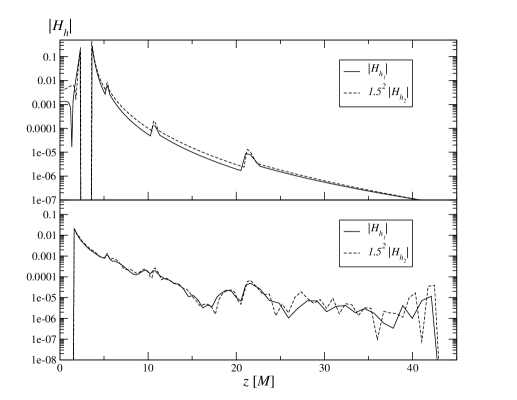
Figure 1: Convergence analysis of the Hamiltonian constraint along the $z$-axis at $t=0$ (upper panel) and $t=25.92\,M$ (lower panel).

In consequence, the constraint violations inherent to the HuMaSh construction are problematic only if they are significant relative to the limit set by finite grid resolutions in the course of the evolution. Furthermore, the constraint violations are reduced as we increase the initial separation of the black holes.

In order to estimate the significance of the constraint violations in the HuMaSh data relative to the numerical evolution errors, we have analyzed the convergence properties of the constraint violations in the course of the simulations. Because the initial data are not exactly constraint satisfying, we do not expect the values of the constraints to converge to zero at second order in the continuum limit. Let $\mathcal{H}_{0}$ denote the Hamiltonian constraint violation at the continuum level inherent to the HuMaSh data. $\mathcal{H}_{0}$ is thus independent of the grid resolution. For a second-order convergent evolution code, the numerical constraint violation $\mathcal{H}_{h}$ will be given by

$$\mathcal{H}_{h}=\mathcal{H}_{0}+c\,h^{2}\,,$$ (10)

where $h$ denotes the grid resolution and $c$ is a function of space and time, independent of $h$. We have carried out two head-on collisions with black holes separated by a coordinate distance $6\,M$. These runs have resolutions $h_{1}=0.135\,M$ and $h_{2}=h_{1}/1.5\,M$ on the finest refinement level respectively, with the grid spacing doubled in each of the three additional coarser levels. (These are the “coarse” and “medium” simulations in the convergence analysis of the waveforms in Sec. IV.2.) For a second-order convergent code we expect the constraint violations at the two resolutions to obey the relation

$$q\equiv\frac{\mathcal{H}_{h_{1}}}{\mathcal{H}_{h_{2}}}=\frac{\mathcal{H}_{0}+c\,h_{1}^{2}}{\mathcal{H}_{0}+c\,h_{2}^{2}}.$$ (11)

It is instructive to consider the following two limiting cases of this equation. First, if the contribution $\mathcal{H}_{0}$ due to the use of initially unsolved data dominates the total constraint violation, we obtain $q=1$ and should observe no convergence at all. On the other hand, if $\mathcal{H}_{0}$ is negligible, we expect second-order convergence and $q=1.5^{2}$.

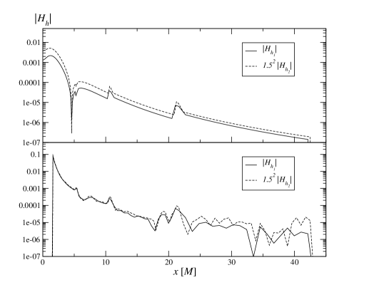
Figure 2: Convergence analysis of the Hamiltonian constraint along the $x$-axis at $t=0$ (upper panel) and $t=25.92\,M$ (lower panel).

In view of this result, we have investigated the point-wise convergence of both the Hamiltonian and the momentum constraints. Fig. 1 shows the Hamiltonian constraint violation $\mathcal{H}_{h}$ along the $z$-axis (collision axis) for both runs, with the medium resolution result ($h_{2}=h_{1}/1.5$) scaled by a factor of $1.5^{2}$. The upper panel shows $\mathcal{H}_{h}$ at $t=0$ and the lower panel at $t=25.92\,M$. It is clear from this figure that at $t=0$ second-order convergence is obtained in the strong field area close to the hole as well as in the far-field limit. At intermediate distances, on the other hand, the convergence deteriorates, in particular near $z=0$, the region between the two holes. In the course of the evolution, however, the convergence approaches second order everywhere except in the domain of influence of the outer boundary, as clearly demonstrated in the lower panel of Fig. 1. The constraint violations are second-order convergent out to about $z=22\,M$. We emphasize that these outer boundary effects are not related to the question of initial data and have also been observed, for example, in the puncture evolutions of Alcubierre et al. Alcubierre et al. (2004a). This viewpoint is further strengthened by the convergence analysis of the waveforms in Sec. IV.2 which also reveal the propagation of noise from the outer boundaries as the limiting factor.

In order to shed more light on the constraint violations at small $z$, we show in Fig. 2 the Hamiltonian constraint violations along the $x$-axis at the same times. Due to the axisymmetry in the problem, the results along the $y$-axis are identical. Clearly the initial data do not exhibit second-order convergence, in agreement with the results of Fig. 1 near $z=0$. In the course of the evolution, however, as the discretization error increases and dominates the total violations we do find second-order convergence of the Hamiltonian constraint except for the outer boundary effects mentioned above.

The results obtained for the momentum constraints show the same behavior, though they exhibit a stronger level of noise emanating from the refinement boundaries. We currently do not have an explanation for this discrepancy between Hamiltonian and momentum constraint but emphasize that the overall convergence of the momentum constraint is still close to second order up to the outer boundary effects.

Similar convergence properties are found for the $\ell_{2}$-norms of the Hamiltonian constraint $\mathcal{H}$, the momentum constraints $\mathcal{M}_{i}$ and the auxiliary constraint $\mathcal{G}^{i}\equiv\tilde{\Gamma}^{i}-\tilde{\gamma}^{jk}\tilde{\Gamma}^{i}_{jk}$. In Fig. 3 we show the resulting plots for the $x$-components $\mathcal{M}_{x}$ and $\mathcal{G}^{x}$. As before, the constraint violations obtained with fine resolution $h_{2}$ are scaled by the expected factor $1.5^{2}$. The results for the other components of the constraint variables are similar and overall we find convergence close to second order after a transition time of about $10\,M$. Outer boundary effects do not manifest themselves as clearly in the $\ell_{2}$-norms as in the point-wise convergence analysis. We attribute this feature to the fact that the norms are dominated by the large constraint violations near the black holes.

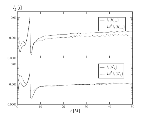
Figure 3: Convergence analysis of the $\ell_{2}$-norms as functions of time of the $x$-component of the momentum and auxiliary constraints.

In summary, our results confirm that the total constraint violation is indeed dominated by the numerical inaccuracies inevitably generated during time evolutions at currently available grid resolutions. This analysis generalizes the studies of Marronetti et al. Marronetti et al. (2000) to include the discretization errors arising from the time evolution; these lead to an extension of the allowed range of grid spacings from their limiting value of $M/4$ to about $M/8$ as used in this work. While constraint solving of the initial data will be desirable for future simulations with higher resolutions, its effect on the overall constraint violations encountered in our simulations would be marginal at most. We emphasize in this context that this is only the case because of the absence of exponentially growing constraint violating modes in our simulations.

III Numerical Evolution

From the operational point of view, it is convenient to divide a black hole head-on collision into pre-merger, merger and post-merger stages. In the pre-merger stage, the evolution contains two separate apparent horizons and therefore separate excision regions. The merger stage is signaled by the appearance of a single, highly distorted apparent horizon. Initially, these deformations of the horizon prevent the merger of the excision masks into a single spherical excision. The end of the merger stage is marked by the merger of excision masks when the deformations of the common apparent horizon have damped-out. The main constraint on the construction of the merged mask is that it must be completely inside the apparent horizon and fully contain the previous two disjoint excision regions. During the final stage (post-merger), the evolution consists of the settling or ring-down of the resulting black hole.

There are certain aspects besides the handling of the excision region, such as gauge conditions, that require a different treatment during each of these stages. Before we discuss these differences in detail, we address those ingredients of the numerical evolution that remain unchanged throughout the complete simulation.

The specific implementation of the 3+1 BSSN formulation and the black hole excision technique used in the Maya code have been described in detail in Paper 1. Here we provide a brief summary with particular regard to the changes necessary for working with fixed-mesh refinement.

We evolve the Einstein equations on a set of nested non-moving, uniform Cartesian grids with the resolution increasing by a factor of two for each additional refinement level. The Einstein field equations are evolved according to the BSSN 3+1 formulation Shibata and Nakamura (1995); Baumgarte and Shapiro (1999). The exact shape of the equations as implemented in the code is given by Eqs. (6)-(10) in Paper 1; in particular this includes the additional term in the evolution of $\hat{\Gamma}^{i}$ introduced by Yo et al. (2002) (the free parameter $\chi$ present in that term is set to $2/3$ for all simulations discussed in this paper). These equations are evolved in time with the iterated Crank-Nicholson scheme. Spatial discretization is second-order centered finite differencing with the exception of advection derivatives contained in the Lie derivatives; these are approximated with one-sided second-order stencils. With regard to the treatment of refinement boundaries, we follow the recipe of Schnetter et al. Schnetter et al. (2004) to avoid loss of convergence at these boundaries. For our code, this implies the use of a total of six buffer zones; two points (because of the one-sided derivatives mentioned above) for each of the three Crank-Nicholson iterations.

With the exception of gauge quantities specified algebraically as functions of the spacetime coordinates, we apply a Sommerfeld-like outgoing condition at the outer boundary Shoemaker et al. (2003). At the excision boundary, we extrapolate all evolution fields from the computational interior using quadratic or, when populating previously excised points, cubic polynomials. With regard to mesh refinement we note that the black hole excision is actively implemented on the finest level, only migrating to the coarser levels via the restriction of grid functions; consequently, we always require that the black holes remain within the range of the finest grid. In practice this is not a limitation since it is precisely the black hole neighborhood where steep gradients are present and high resolution is therefore required.

In Paper 1, the uni-grid version of this code has been shown to produce long-term-stable evolutions of single Schwarzschild black holes as well as evolutions of moving black holes lasting for about $130\,M$. In Sperhake et al. (2004) (referred to as Paper 2 from now on), we managed to extend the life times of these runs to at least $6000\,M$ by describing the slicing condition in terms of a densitized lapse function [cf. Eqs. (6)-(8) therein] and demonstrated second-order convergence of the code.

The remaining aspects of the numerical simulation are specific to the individual stages of the evolution and will now be discussed in turn. The main differences encountered here have to do with gauge and excision.

III.1 Pre-Merger Evolution

Pre-merger, our spacetime contains two apparent horizons. Within each apparent horizon, there is a curvature singularity, hidden from us by singularity excision. As the holes approach each other, the excised regions – or excision masks – are allowed to move also. The new locations of the excision masks must be found by somehow tracking the locations of the black hole singularities. One possibility is to track the singularities via an apparent horizon finder; we have found, however, that a simple Gaussian fit to the shape of the trace of the extrinsic curvature is equally effective for this purpose. As the excision regions move, grid points that were previously excised become part of the computational domain. These uncovered points must be supplied with valid data for all fields; this “re-population” of points is achieved through extrapolation onto the mask surface along coordinate normals to the surface. Both the Gaussian mask tracking and the re-population procedure have been treated in detail in Papers 1 and 2.

Besides the above, the current problem of evolving binary data raises new challenges. Primary among these is the question of gauge conditions. While substantial progress has been made in the recent past in deriving successful gauge conditions for evolutions that anchor black holes to a fixed coordinate location (see e. g. Bona et al. (1995); Alcubierre and Brügmann (2001); Alcubierre et al. (2001b); Yo et al. (2002); Alcubierre et al. (2003b, c); Brügmann et al. (2004)) the question as to suitable gauge conditions for strongly time varying scenarios, such as spacetimes with moving black holes, remains largely unanswered.

In view of the successful simulations of single moving black holes in Paper 2, we have decided to pursue a similar approach for the binary system at hand, namely analytic shift and densitized lapse. A key benefit of using a densitized version of the lapse is that it facilitates an algebraic specification of the slicing condition, in terms of an analytic function of the spacetime coordinates, while satisfying criteria for strong and symmetric hyperbolicity as derived in Gundlach and Martín-García (2004) or Sarbach et al. (2002). Using a densitized lapse thus leads to a well-posed Cauchy problem as defined in Nagy et al. (2004). In contrast to the single black hole simulations of Paper 2, where algebraic forms of the shift and densitized lapse were available from the analytic single black hole solution, gauge conditions for our head-on collisions, in which the black holes exhibit changes in their coordinate location, require a suitable guess. We must emphasize that any gauge condition we introduce should not in principle affect the physical content in the spacetime. In practice, we specify gauge conditions that facilitate the merger and achieve long-term-stable evolutions.

We require that the lapse function and shift vector resemble those of a single, boosted Kerr-Schild black hole in the vicinity of each singularity, namely Eqs. (3) and (4) respectively. Using these single, boosted black hole expressions, we construct the following gauge conditions:

$$Q = \gamma^{-1/2}\left(\,{}^{A}\alpha^{-2}+\,^{B}\alpha^{-2}-1\right)^{-\frac{1}{2}},$$ (12)

$$\beta^{i} = \gamma^{ij}\left(\,{}^{A}\beta_{j}+\,^{B}\beta_{j}\right).$$ (13)

Here $Q$ represents the densitized lapse, $\gamma_{ij}$ is the analytic three-metric given in Eq. (8), $\gamma$ its determinant and $\,{}^{A}\alpha$, $\,{}^{B}\alpha$, $\,{}^{A}\beta_{j}$, $\,{}^{B}\beta_{j}$ are the analytic lapse and covariant shift of holes $A$ and $B$. It is not difficult to show that the expressions (12) and (13) have a close limit. That is, at zero separation and boost velocity, they coincide with the densitized lapse and shift of a single, non-rotating, non-boosted Kerr-Schild hole of mass $M=2m$.

It is important to emphasize that the gauge conditions (12) and (13) require information about the coordinate location of the black hole singularities and boost velocities. Here, black hole coordinate location is not meant to be a formal statement about the precise location of the physical singularities, but it is merely used to represent the point with respect to which (12) and (13) are evaluated. Therefore, in order to use these gauge conditions, there remains the task of finding suitable trajectories for the black holes. We have found the following “Newtonian” trajectories adequate for this purpose:

$$\vec{r}(t)=\vec{r}_{0}+\vec{v}_{0}t+\frac{1}{2}\vec{a}_{0}t^{2}\,.$$ (14)

Here $\vec{r}_{0}$ and $\vec{v}_{0}$ are the initial singularity position and boost velocity, respectively. The value for $\vec{a}_{0}$ is obtained iteratively using a small number of preliminary runs to ensure the largest gradients of the gauge fields remain well covered by the excision mask. During the evolution, the boost velocity needed to compute (12) and (13) is obtained simply from $\vec{v}=d\vec{r}/dt$.

III.2 The Merger of Excision Masks

The key point during the merger stage is, once a common apparent horizon has formed and been identified, to replace the individual spherical excision masks with a single spherical one. The size of this new excision region is determined by the minimum sphere containing the original excision masks. However, special care must be taken with regard to the timing of this replacement. One must check that the new spherical mask is fully contained within the apparent horizon. Typically, when the common horizon forms, it has an elongated or prolate shape. Therefore, a delay in merging the mask allows the common apparent horizon to become more spherical, thus facilitating the creation of a spherical merged mask. On the other hand, there is a constraint on how long this delay can be. Because of the extrapolations involved in the excision, one cannot delay the merger of the masks until their surfaces touch each other. Even if the common apparent horizon is not completely spherical, the masks are merged if there are not enough grid-points between the individual masks to carry out excision extrapolations. Of course, in this case one still has to continue to satisfy the requirement that the merged mask is contained within the apparent horizon. For the head-on collisions under consideration, we find that the common apparent horizon becomes almost spherical before the separation of individual masks decreases to the point of preventing excision extrapolations.

Resolution also plays a factor during the mask merger. If the grid resolution in the vicinity of the black holes is too coarse, the minimum coordinate separation of the individual masks required by excision extrapolations will be too large. In consequence, it becomes more difficult to find a spherical merged mask that comfortably fits within the common apparent horizon. For the typical resolution used in our simulations, $h=0.135\,M$, two single-hole masks of radius $0.405\,M$ require a merged mask with radius of $1.1475\,M$. That is, single-hole masks with 40.5 % of the single-hole horizon radius mean the new excision radius is approximately 57 % of the common horizon radius.

III.3 Post-Merger Ring-Down

After the excision mask merger, the key change concerns the gauge conditions. Post-merger, the spacetime effectively represents a single ringing black hole, and the problem at hand is similar to that of evolving a single stationary hole. In Papers 1 and 2, we have demonstrated how this scenario can be simulated with long-term stability using either live gauge conditions or algebraic gauge using a densitized lapse. The same options apply to the post-merger stage of a black hole collision, and we have found that either approach provides long-term stability. For the extraction of wave forms, we find a similar situation: live and densitized algebraic gauge conditions generate waveforms that differ only within numerical errors. For simplicity, we use densitized algebraic gauge conditions (see Paper 1 and 2 for details).

There remains the question of how the transition from the superposed gauge (12) and (13) to a single black hole gauge takes place. As mentioned before, the gauge conditions (12) and (13) have the correct close limit (i.e. vanishing separation and boost velocities). Starting at the time when the masks are merged, we match the current “black hole positions” given by (14) to decelerating trajectories given by sixth-order polynomials in time. These new trajectory functions are such that the coordinate separation and boost velocities vanish within a time interval (typically $10\,M$). The order of the polynomial is fixed by requiring continuity of the boost velocity and acceleration.

IV Results

The spacetime of head-on collisions of non-spinning black holes is by construction axisymmetric. In the equal-mass case there is a further reflection symmetry across the plane perpendicular to the collision axis halfway between the holes. Although the simulations in this work are intrinsically 3D, we take advantage of these symmetries and evolve only one octant of the numerical domain. One of the primary goals of our work is to perform 3D-simulations of head-on collisions with initial separations never tried before. However, determining what constitutes a large separation has the following complication. Previous work on head-on collisions has used exclusively Misner or Brill-Lindquist initial data, as for example the recent long-term-stable simulations of Alcubierre et al. Alcubierre et al. (2003a, 2004a). To our knowledge, the only evolutions of binary Kerr-Schild (HuMaSh) data is the grazing collision of Brandt et al. Brandt et al. (2000), where the black holes had an initial coordinate separation of $5\,M$.

We must emphasize that there exists no unambiguous definition of a black hole separation; also, given that we are using HuMaSh initial data, direct comparison of our initial black hole coordinate separations with those from Misner or Brill-Lindquist initial data is not correct. An operational measure of higher physical significance is given by the horizon-to-horizon proper separation. That is, the proper 3D distance horizon-to-horizon computed along the collision axis within the hypersurface where the initial data resides. One should bear in mind that this proper separation is slicing-dependent. Additionally, our proper distance separation suffers from the effects due to constraint violations intrinsic to the HuMaSh data.

Table 1 gives the black hole coordinate ($D$) and proper ($L$) separations for the two sets of runs (labeled $D06$ and $D10$) performed in this work. In addition, the table gives the initial boost velocity ($v_{0}$) as well as the “acceleration” parameter ($a_{0}$) used to compute the trajectories required to construct the gauge variables [cf. Eq. (14)]. As a reference, the “Cook-Baumgarte” ISCO Baumgarte (2000); Cook (1994) corresponds to a proper separation between $4.8$ and $4.88\,M$. Similarly, the orbit simulation by Brügmann et al. Brügmann et al. (2004) started from a proper separation of about $9\,M$.

We evolve the initial data on a set of four nested refinement levels, with resolution and extent as given in Table 2. Except for the outermost level, grid spacing and extent always increase by a factor of two. We have found that a grid spacing significantly larger than $1.08\,M$ in the outer regions gives rise to substantial reflections of gravitational waves at the refinement boundary. For this reason we have pushed the outermost level to $140.4\,M$ without adding a further coarser level.

Table 1: Setup parameters for the runs. $D$ and $L$ are the coordinate and proper initial separations. $v_{0}$ is the boost velocity and $a_{0}$ the “acceleration” parameter to compute the gauge trajectories.

Run	$D\,[M]$	$L\,[M]$	$v_{0}$	$a_{0}\,[M^{-1}]$
$D06$	$6$	$5.49$	$0.289$	$0.040$
$D10$	$10$	$10.06$	$0.270$	$0.014$

Table 2: Grid parameters of the refinement levels used in the simulations. The number of grid points $N$ includes ghost, symmetry and outer boundary zones. $r_{\rm max}$ is the extent in the $x$, $y$ and $z$-directions.

ref-level	$h\,\,[M]$	$N$	$r_{\rm max}\,\,[M]$
1	$0.135$	$67^{3}$	$8.505$
2	$0.27$	$67^{3}$	$17.01$
3	$0.54$	$67^{3}$	$34.02$
4	$1.08$	$134^{3}$	$140.4$

Using the setup described above, we obtain long-term-stable evolutions. The three simulation stages described in Sec. III are illustrated in Fig. 4. This figure contains snapshots of the $D10$ run at times $t=0$, $10.8\,M$ and $14\,M$, including the marginally trapped surfaces as calculated by Thornburg’s AHFinderDirect code Thornburg (1996, 2004).

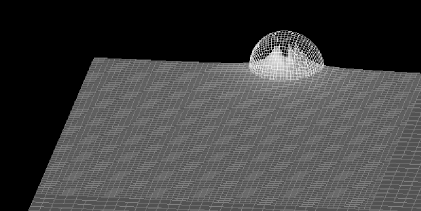
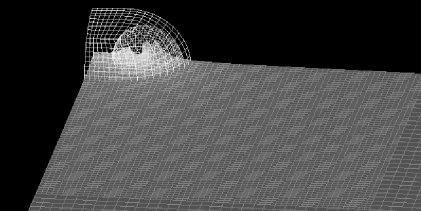
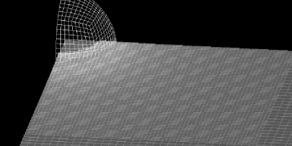
Figure 4: Snapshots of the $D10$ run taken at times $t=0$, $10.8$ and $14\,M$. From top to bottom the panels show the individual holes with distinct apparent horizons (only one hole is visible due to the octant symmetry), a common apparent horizon forming around the individual trapped surfaces and a single apparent horizon surrounding a single excision region.

The upper panel shows the initial configuration with holes present at $z=\pm 5\,M$. As mentioned above the computational domain only includes the hole at $5\,M$ due to symmetry. During this pre-merger stage each hole is surrounded by its own apparent horizon (AH). In the middle panel, the holes are sufficiently close to one another that a common AH has formed. However, as mentioned before, it is not possible yet to switch to a single excision region because of the elongated shape of the common apparent horizon. The lower panel shows the beginning of the post-merger stage.

IV.1 Waveforms

We extract waveforms at radii $12.5$, $20$, $25$ and $30\,M$ using the Zerilli-Moncrief formalism; details are given in App. A. In principle, it is desirable to extract gravitational waves at large radii so as to ensure that the assumptions inherent to the Zerilli-Moncrief extraction are satisfied. We observe two problems, however, which arise out of choosing excessively large radii. First, outer boundary effects require less time to propagate inward and reach the extraction radius. Second, the actual wave signal contained in the metric and curvature variables is weaker at larger radii and thus requires higher accuracy in the numerical evolution. In combination with the increasingly coarse resolution used in outer levels, this gives rise to a degree of distortion and noise in the extracted Zerilli function which is not present at smaller radii. We find the values used above to be a reasonable compromise for the post-merger stage of the head-on collision.

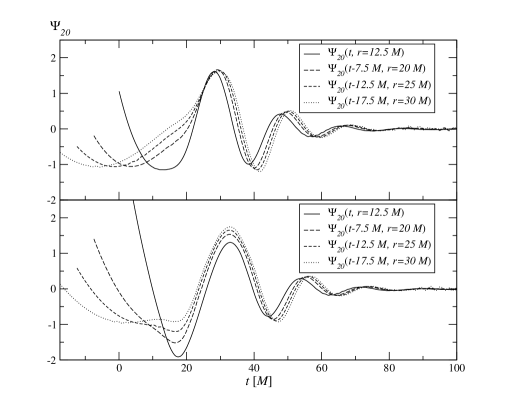
Figure 5: The $\ell=2,m=0$ Zerilli function extracted at different radii for the $D06$ (upper panel) and $D10$ (lower panel) runs. The curves have been shifted in time by the difference in propagation time of the wave signal between the different radii.

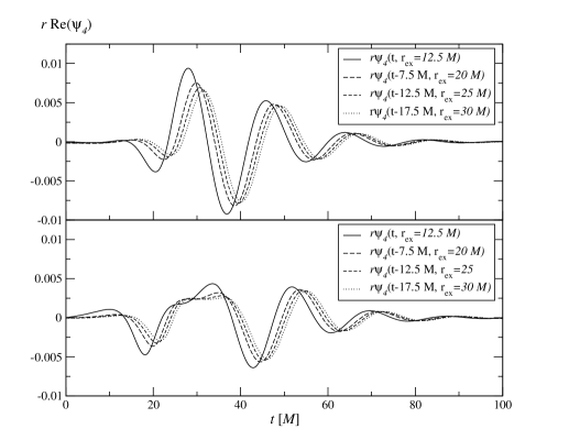
Figure 6: The $\ell=2$, $m=0$ component of the real part of the Newman-Penrose scalar $\psi_{4}$ extracted at different radii for the $D06$ (upper panel) and $D10$ (lower panel) runs. The curves have been shifted in time by the difference in propagation time of the wave signal between the different radii.

In Fig. 5 we show the resulting $\ell=2,m=0$ waveforms, each shifted in time by the amount required by the signal to travel from $r=12.5\,M$ to the corresponding extraction radius. All curves in the figure show a significant initial signal up to about $t\approx 10\,M$. We trace the origin of this signal to the fact that the two black holes are far apart in the early stages of the simulation and thus the assumption underlying the wave extraction technique, namely that the spacetime is that of a single black hole plus a perturbation, is not satisfied with sufficient accuracy during the pre-merger phase. This viewpoint is strengthened by the observation that the spurious signal is stronger for the larger black hole separation of case $D10$ in the lower panel of the figure. We further note in this context that the merger of the black holes occurs at $t=5.4\,M$ and $11.75\,M$ respectively for cases $D06$ and $D10$. It is at about these times that the shifted waveforms extracted at different radii start showing better agreement with each other in the figures, while the spurious signal present at earlier times converges away at larger extraction radii.

Because the Zerilli potential becomes zero in the limit of infinite extraction radii, one would expect the curves in the individual panels of Fig. 5 to overlap exactly in this limit. The figure shows that this criterion is satisfied with increasing accuracy at larger radii. Still there remain small effects of back-scattering of the wave signal at the finite radii used in the extraction. The figure also reveals some noise developing at late times at larger radii; an analysis of the timing of the noise demonstrates that these are boundary effects propagating inward. Below, we will see that these effects limit the convergence properties of our code and thus the reliability of the results after the onset of noise in the waveforms.

An alternative to the Zerilli-Moncrief approach to wave extraction is provided by the Newman-Penrose scalar $\psi_{4}$. Given the Weyl tensor $C_{abcd}$, and an appropriately chosen null tetrad $\{l,n,m,\bar{m}\}$, $\psi_{4}\equiv C_{abcd}\,\bar{m}^{a}\,n^{b}\,\bar{m}^{c}\,n^{d}$ represents a measure of the outgoing gravitational wave content. We calculate $C_{abcd}$ using the “electric-magnetic” decomposition Smarr (1975) as described in Gunnarsen et al. (1995). For spacetimes perturbatively close to Kerr, the appropriate choice of null tetrad is the Kinnersley tetrad Kinnersley (1969) In practice, the exact Kinnersley tetrad is not available in a numerical simulation. Even though recent work has suggested that it may be possible to identify unambiguously the Kinnersley null directions of the numerical spacetime Beetle et al. (2004), the resulting Weyl scalars would still differ from their Kinnersley values in polarization and scaling. For simplicity we use instead a symmetric null tetrad formed from an orthonormalized spherical coordinate tetrad:

$$l^{a}\equiv\frac{1}{\sqrt{2}}\,(u^{a}+e_{r}^{a})\,,\, n^{a}\equiv\frac{1}{\sqrt{2}}\,(u^{a}-e_{r}^{a})\,,$$ (15)

$$m^{a}\equiv\frac{1}{\sqrt{2}}\,(e_{\theta}^{a}+i\,e_{\phi}^{a})\,, \bar{m}^{a}\equiv\frac{1}{\sqrt{2}}(e_{\theta}^{a}-i\,e_{\phi}^{a}).$$

Here $u$ is the future-pointing unit hypersurface normal and the coordinate triad vectors were orthonormalized via a Gram-Schmidt process in the order $e_{r}$, $e_{\theta}$, $e_{\phi}$. A symmetric tetrad of this kind (though possibly orthonormalized in a different order) is a standard choice in approximately spherically symmetric spacetimes Smarr (1979); Zlochower et al. (2005); Fiske et al. (2005), and is the starting point of the Lazarus procedure Baker et al. (2002). While the numerical three-metric is used for orthonormalization, the tetrad requires no explicit knowledge of a background spacetime, and so the resulting expressions do not involve parameters such as a background mass and angular momentum. At large extraction radii, the leading difference between these tetrad components will be an overall (radius-dependent) scaling factor, which is not relevant for our purposes. Additionally, any coordinate distortion should be a first- order effect, and should not influence the waveforms to leading order. That said, we cannot quantify the relative strength at early times of the assumptions behind Weyl extraction of this type and Zerilli extraction as described earlier.

In Fig. 6 we plot the $\ell=2$, $m=0$ quadrupole moment of the real part of $r\psi_{4}$. The application of the factor $r$ is convenient because the resulting function will propagate in the limit of large radii in analogy to the Zerilli function. While the waveforms in Figs. 5, 6 exhibit good agreement during the merger and ring-down phase, differences are apparent during the early in-fall stage. In particular the Newman-Penrose waveform is less severely affected by the deviations from an approximately spherically symmetric spacetime. While a detailed comparison between the two methods of gravitational wave extraction is beyond the scope of this work, it will be interesting to analyze the observed discrepancies in more depth in future work. The same applies to the distortion visible in the Newman-Penrose waveform for the simulation $D10$ around $t=30\,M$.

In the remainder of this work we will restrict our analysis to the waveforms of Fig. 5 obtained with the Zerilli-Moncrief formalism. In order to estimate the quality of the waveforms, next we investigate their convergence properties.

IV.2 Convergence

The discretization of the BSSN-evolution equations in the Maya code is implemented with second-order accuracy in the grid spacing $h$. The wave extraction, as described in Appendix A, involves numerical approximations of higher-order accuracy, such as the interpolation of grid functions onto the sphere of extraction and the evaluation of the integrals over the spheres. The numerical error in the wave functions should therefore be dominated by the second-order accuracy of the evolution of the field equations, and we expect the wave forms to exhibit second-order convergence.

In order to verify this numerically, we focus our attention on the head-on collision case $D06$ and carry out two additional runs. Compared with the resolutions listed in Table 2, the two additional runs are finer by factors of $1/1.5$ and $1/1.5^{2}$. On the finest grid for each of the three runs, this leads to resolutions $h_{1}=0.135\,M$, $h_{2}=0.09\,M$ and $h_{3}=0.06\,M$, respectively. Because the coarsest mesh in $D06$ has an extent of $140.2\,M$, implementing the $1/1.5$ and $1/1.5^{2}$ refinements far exceeds the available memory of our hardware resources. For this reason, instead of using mesh-refinements with the sizes given in Table 2, we have performed the convergence analysis using for each run four refinement levels of extent $r_{\rm max}=5.4$, $10.8$, $21.6$ and $43.2\,M$. The key difference compared with the simulations discussed above is that outer boundary effects will reach the extraction radii at earlier times. To mitigate this effect we extract the Zerilli function at the smaller radius $r_{\rm ex}=7.5\,M$ for this analysis.

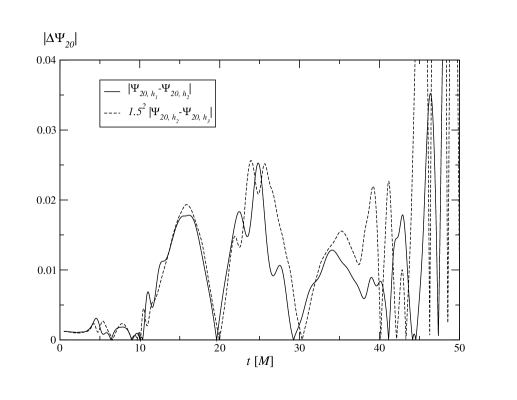
Figure 7: Three-level convergence analysis for the $\ell=2$, $m=0$ Zerilli function extracted at $r=7.5\,M$.

In Fig. 7 we show the difference in the $\ell=2$, $m=0$ Zerilli function obtained for the three different resolutions. The difference in $\Psi_{20}$ between the medium and high resolution runs has been amplified by the factor $1.5^{2}$ expected for second-order convergence. The resulting curve agrees reasonably well with the difference obtained from using the low and medium resolution until about $35\,M$, indicating second-order convergence. After that time, noise originating from the outer boundary at $43.2\,M$ has reached the extraction radius at $7.5\,M$ and spoils the convergence properties. This result is confirmed by analysis at larger radii where second-order convergence is observed for correspondingly shorter periods of time. We conclude that our code facilitates second-order convergent wave extraction until outer boundary effects have had the time to propagate inward toward the radius of wave extraction. For the simulations presented in the previous subsection, this result implies reliable waveforms up to a time of about $100-125\,M$ depending on the extraction radius.

In view of this result it appears desirable to achieve more satisfactory boundary treatments. Various alternatives have been suggested to this effect in the past. Conceptually the most elegant approach consists in the incorporation of null-infinity in the numerical domain via the so-called Cauchy-characteristic matching. The key feature of this technique is the matching of a “3+1” formulation in the interior regions containing the strong-field sources to a characteristic formulation of the exterior spacetime (see e. g. Bishop et al. (1996); d’Inverno and Vickers (1996); Winicour (2001)). This facilitates a straightforward compactification of the spacetime and, thus, the implementation of exact boundary conditions. An alternative matching technique has been suggested in Abrahams et al. (1998). Here the weak-field exterior spacetime is described in terms of non-spherical perturbations of a Schwarzschild background. A different strategy without matching involves the development of alternative boundary conditions which by construction preserve the constraint equations (see e. g. Frittelli and Gómez (2004); Gundlach and Martín-García (2004); Beyer and Sarbach (2004)). While the derivation of such boundary conditions has largely been motivated by stability issues, it would be interesting to see their effect on spurious reflections as observed in our simulations. The implementation of either of these alternative boundary treatments represents a considerable challenge, however, and is beyond the scope of this work. Instead we reduce the impact of boundary effects by placing the outer boundaries far from the strong field sources.

Finally we emphasize that in spite of the accuracy limitations arising from our implementation of the boundary conditions, we have not observed any sign of instabilities: all simulations presented in this work have continued for many hundreds or even thousands of $M$ gradually approaching a stationary spacetime containing a single black hole.

IV.3 Quasi-normal Ringing, Masses and Radiated Energy

Table 3: Quasi-normal ringing damping $\sigma$ and oscillation frequency $\omega$ measured from the extracted waveforms. The final column gives the percentage of the initial ADM mass radiated away in the form of gravitational waves as derived from Eq. 17

run	$r_{\rm ex}/M$	$\sigma M_{\rm ADM}$	$\omega M_{\rm ADM}$	$E_{\rm rad}\,[\%]$
$D06$	$12.5$	$0.0917$	$0.365$	$0.20$
$D06$	$20$	$0.0921$	$0.362$	$0.15$
$D06$	$25$	$0.0923$	$0.363$	$0.14$
$D06$	$30$	$0.0947$	$0.366$	$0.14$
$D10$	$12.5$	$0.0973$	$0.369$	$0.37$
$D10$	$20$	$0.0963$	$0.363$	$0.16$
$D10$	$25$	$0.0960$	$0.365$	$0.14$
$D10$	$30$	$0.0976$	$0.366$	$0.13$

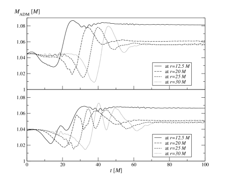
Figure 8: ADM mass as a function of time evaluated at various radii for the $D06$ (upper panel) and $D10$ (lower panel) simulation.

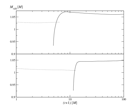
Figure 9: The apparent horizon mass as a function of time calculated for the $D06$ (upper panel) and $D10$ (lower panel) simulation.

Previous studies have shown that most of the gravitational radiation of a head-on collision is emitted in the post-merger ring-down phase, with the total radiated energy typically being less than a percent of the total initial mass Anninos et al. (1993); Price and Pullin (1994); Abrahams and Cook (1994); Anninos et al. (1995b). Furthermore, the quasi-normal ringing of the post-merger black hole is dominated by the $\ell=2$, $m=0$ mode with small contributions from the $\ell=4$, $m=0$ multipole. Our simulations represent the first head-on collisions with wave extraction using Kerr-Schild type data. They are in good agreement with the picture described above.

We first note that up to $\ell=3$ the only multipole with a notable wave signal is the $\ell=2$, $m=0$ quadrupole shown in Fig. 5. Second, we have performed least-square fits of the waveforms to

$$f(t)=A\,e^{-\sigma t}\cos\,(\omega t-\phi_{0}).$$ (16)

in order to calculate the ringing damping $\sigma$ and oscillation frequency $\omega$. The results are given in Table 3. The resulting damping and oscillation frequency values agree within about $10\,\%$. For comparison, the quasi-normal mode spectrum of the Schwarzschild black hole calculated by Chandrasekhar and Detweiler Chandrasekhar and Detweiler (1975) predicts $\sigma\mathcal{M}=0.0890$, $\omega\mathcal{M}=0.374$, where $\mathcal{M}$ denotes the mass associated with the black hole background spacetime. In Table  3, the results are reported in units of the total initial ADM mass $M_{\rm ADM}$. The differences between these two masses are the radiated energy and numerical errors.

In the course of the evolution we numerically approximate the ADM mass by evaluating the ADM integral at finite extraction radii. The result is shown in Fig. 8 for simulation $D06$ in the upper panel and $D10$ in the lower panel. The initial values agree well with the sum $\gamma M$ of the special relativistic masses of the two individual holes moving with the velocities given in Table 1, that is $M_{\rm ADM}=1.045\,M$ and $1.039\,M$ respectively. During the evolution the numerical ADM mass remains within a few percent of the initial value but in contrast to intuitive expectations it increases slightly rather than decreases after the gravitational waves have passed the extraction radius. Even though this increase becomes less pronounced at larger extraction radii we do not consider this calculation of the ADM mass sufficiently accurate to support a calculation of the total radiated gravitational wave energy from conservation arguments.

In Fig. 9, we plot the apparent horizon masses as calculated by AHFinderDirect for the two cases $D06$ (upper) and $D10$ (lower panel). During the pre-merger stage there is no common apparent horizon present and we plot instead the sum of the horizon masses associated with the individual holes (dotted curves). In contrast the solid curve represents the horizon mass of the single post-merger hole. In the early stages after merger the horizon mass shows a significant increase in time but quickly settles down in the final values of $1.06\,M$ and $1.05\,M$ respectively. These values show good agreement with the values $1.045\,M$ and $1.039\,M$ used for the black hole background mass for the wave extraction. Theoretically one would not expect the horizon mass to decrease as a function of time. We attribute the decrease by about one percent visible after the merger in the upper panel of Fig. 9 to numerical inaccuracies.

We estimate the total radiated energy from the Landau-Lifshitz formula (see e. g. Cunningham et al. (1980)) which gives the radiated power as

$$\rm P=\frac{1}{96\pi}\Psi_{,t}^{2},$$ (17)

where the constant factor arises from our definition of the Zerilli function in Eq. (23). Ideally this function needs to be evaluated at null infinity. As this is not possible in this type of computation, we approximate the exact result by calculating the radiated energy at various finite radii. For this purpose, we have evaluated the integral of ${\rm P}$ from $t=0$ to $t=140\,M-r_{\rm ex}$; that is, we have excluded late times when the extraction radius is causally connected to the outer boundary. The results are shown in the last column of Table 3 and show the impact at small extraction radii of the spurious signal in the Zerilli function at early times when the two holes are still far apart from each other. This feature leads to an overestimate of the radiated energy but quickly converges away if we extract at larger radii. A close investigation reveals that this spurious contribution drops to a few percent of the total radiated energy at $r_{\rm ex}=30\,M$ in the case $D10$ and even less in the case $D06$. Within these error bounds we thus find a radiated energy of about $0.14$ and $0.13$ percent of the total ADM mass of the system.

V Conclusions

We have presented the first long-term-stable binary black hole collisions with wave extraction using fixed mesh-refinement, Kerr-Schild type initial data and dynamical excision. While the success of our dynamical excision technique has been demonstrated in the past in the case of static and dynamic single black hole spacetimes, the results in the present work demonstrate the applicability of our dynamical excision to binary black hole systems with gravitational wave generation.

Our simulations start from initial data constructed via superposition of two single Kerr-Schild black holes, namely HuMaSh data. We have demonstrated by convergence analysis of the Hamiltonian and momentum constraints that the inherent constraint violations in the HuMaSh data is not significant compared with the level of accuracy allowed by current computational resources.

We have conceptually divided the evolutions into three stages: the initial in-fall, the merger and the post-merger ring-down of the resulting single black hole. In particular during the first two stages, special care must be taken to ensure that the excision region always be entirely contained inside the apparent horizon. For this purpose, we have calculated the apparent horizon at each time step and verified that no causal violation of the excision technique occurs.

We have extracted gravitational waves using the Zerilli-Moncrief approach applied to a black hole background spacetime in Kerr-Schild coordinates. Our results confirm previous findings. Wave emission is dominated by the quasi-normal ringing of the single post-merger black hole. Up to $\ell=3$ the only notable contribution is the $\ell=2$, $m=0$ quadrupole. Comparison of the damping and oscillation frequencies with analytic results shows good agreement. We do not find the accuracy in calculating the ADM or the apparent horizon mass sufficient, however, to support a calculation of the total radiated gravitational wave energy purely from conservation principles. Instead, we use the Landau-Lifshitz formula to calculate the radiated energy from the Zerilli function. We find this energy to be of the order of $0.1\,\%$ of the ADM mass. Our results demonstrate the need to extract gravitational radiation at sufficiently large radii in order to facilitate reasonable accuracy. In particular, we observe a spurious wave signal in the Zerilli function caused by a systematic deviation during the early pre-merger stage of the numerical spacetime from a perturbed single black hole spacetime. The wave contribution due to this spurious feature converges away as the extraction is carried out at larger radii.

We have also calculated the Newman-Penrose scalar $\psi_{4}$ as an alternative measure of the emitted gravitational radiation. While the results qualitatively confirm those obtained using the Zerilli approach during the merger and ring-down phase, differences are apparent during the early fall-in phase. In particular we find the Newman-Penrose waveforms to be less severely affected by the deviations from an approximately spherically symmetric spacetime at early stages. On the other hand the Newman-Penrose scalar $\psi_{4}$ shows some distortion in the case of larger initial separation of the holes. In future work we plan to investigate in more detail the causes of these distortions as well as compare the different wave extraction techniques and their discrepancies at early stages.

Appendix A Wave extraction using the Zerilli-Moncrief formalism

Our extraction of gravitational waves is based on the gauge invariant perturbation formalism of Moncrief Moncrief (1974). A more detailed description of how this facilitates the extraction of gravitational waves from numerical simulations is given in Abrahams and Evans (1990). Applications of this method can be found, for example, in Anninos et al. (1995b), Abrahams et al. (1992), Camarda and Seidel (1999) or Font et al. (2002).

The key idea is that at sufficiently large distance from a strong field source, the spacetime metric $g_{\mu\nu}$ can be viewed as a spherically symmetric background plus non-spherical perturbations which obey the Regge-Wheeler equation (odd) and the Zerilli equation (even parity perturbations) respectively. In our case the background will be given by that of a single, non-rotating black hole in Kerr-Schild coordinates. Strictly speaking, the coordinates are ingoing-Eddington-Finkelstein coordinates, namely Kerr-Schild coordinates in the case of a non-rotating black hole. The symmetry properties of an equal mass head-on collision imply that the odd perturbations vanish, so we will restrict our attention to the even parity case.

Given the Kerr-Schild background metric

$$g^{\rm B}_{\mu\nu}dx^{\mu}dx^{\nu} = -\left(1-\frac{2\mathcal{M}}{r}\right)dt^{2}+\frac{4\mathcal{M}}{r}dt\,dr$$ (18)

$$+\left(1+\frac{2\mathcal{M}}{r}\right)dr^{2}+r^{2}d\Omega\,,$$

the first-order metric perturbations, expanded in Regge-Wheeler tensor harmonics Regge and Wheeler (1957), can be written as

$$h_{\mu\nu}=\sum_{\ell m}h^{\ell m}_{\mu\nu},$$ (19)

where

$$h^{\ell m}_{\mu\nu}=\begin{pmatrix}H^{\ell m}_{0}Y_{\ell m}&H^{\ell m}_{1}Y_{\ell m}&h^{\ell m}_{0}\partial_{\theta}Y_{\ell m}&h^{\ell m}_{0}\partial_{\phi}Y_{\ell m}\\[10.0pt] {\rm Sym}&H^{\ell m}_{2}Y_{\ell m}&h_{1}^{\ell m}\partial_{\theta}Y_{\ell m}&h_{1}^{\ell m}\partial_{\phi}Y_{\ell m}\\[10.0pt] {\rm Sym}&{\rm Sym}&r^{2}\left(K^{\ell m}+G^{\ell m}\partial_{\theta\theta}\right)Y_{\ell m}&r^{2}G^{\ell m}\left(\partial_{\theta}-\cot\theta\right)\partial_{\phi}Y_{\ell m}\\[10.0pt] {\rm Sym}&{\rm Sym}&{\rm Sym}&r^{2}\sin^{2}\theta\left[K^{\ell m}+G^{\ell m}\left(\cot\theta\,\partial_{\theta}+\sin^{-2}\theta\,\partial_{\phi\phi}\right)\right]Y_{\ell m}\end{pmatrix}.$$ (20)

Here the spherical harmonics $Y_{\ell m}(\theta,\phi)$ form a complete orthonormal system and are eigenvectors of the operator $-\left[\partial_{\theta\theta}+\cot\theta\partial_{\theta}+\sin^{-2}\theta\partial_{\phi\phi}\right]$ with eigenvalue $\ell(\ell+1)$. A straightforward calculation shows that the following linear combinations of the perturbation functions are invariant under first-order coordinate transformations

$$q_{1}^{\ell m} = \frac{2\mathcal{M}r^{2}}{r-2\mathcal{M}}\partial_{t}K^{\ell m}+r\frac{r-3\mathcal{M}}{r-2\mathcal{M}}K^{\ell m}-\frac{4\mathcal{M}^{2}}{r-2\mathcal{M}}H^{\ell m}_{0}$$

$$+r^{2}\partial_{r}K^{\ell m}-(r-2\mathcal{M})H^{\ell m}_{2}-4\mathcal{M}H^{\ell m}_{1},$$

$$q_{2}^{\ell m} = 2h^{\ell m}_{1}+\frac{4\mathcal{M}}{r-2\mathcal{M}}h^{\ell m}_{0}-r^{2}\partial_{r}G^{\ell m}-\frac{2\mathcal{M}r^{2}}{r-2\mathcal{M}}\partial_{t}G^{\ell m}$$ (21)

$$-\frac{r^{2}}{r-2\mathcal{M}}K^{\ell m}.$$

The linearized Einstein field equations are then equivalent to two equations expressed in terms of these gauge invariant variables. The first of these equations is the constraint

$$\left(\partial_{r}+2\frac{\mathcal{M}}{r-2\mathcal{M}}\partial_{t}\right)\left[\left(1-\frac{2\mathcal{M}}{r}\right)(2q_{1}+\ell(\ell+1)q_{2})\right]=0.$$ (22)

The second equation is more conveniently written in terms of the Zerilli function defined in terms of the gauge invariant variables by

$$\Psi_{\ell m}=\frac{-2(r-2\mathcal{M})}{[\ell(\ell+1)-2]r+6\mathcal{M}}[2q^{\ell m}_{1}+\ell(\ell+1)q^{\ell m}_{2}],.$$ (23)

This function represents the dynamical degree of freedom of the polar perturbations of the black hole and obeys the second independent combination of the Einstein equations

$$\left(1+\frac{2\mathcal{M}}{r}\right)\partial_{tt}\Psi_{\ell m}-4\frac{\mathcal{M}}{r}\partial_{tr}\Psi_{\ell m}-\left(1-\frac{2\mathcal{M}}{r}\right)\partial_{rr}\Psi_{\ell m}+\frac{2\mathcal{M}}{r^{2}}(\partial_{t}\Psi_{\ell m}-\partial_{r}\Psi_{\ell m})+V_{\ell}\Psi_{\ell m}=0,$$ (24)

with the potential

$$V_{\ell}=\frac{\ell(\ell+1)[\ell(\ell+1)-2]^{2}r^{3}+6[\ell(\ell+1)-2]^{2}\mathcal{M}r^{2}+36[\ell(\ell+1)-2]\mathcal{M}^{2}r+72\mathcal{M}^{3}}{r^{3}\{[\ell(\ell+1)-2]r+6\mathcal{M}\}^{2}}.$$ (25)

This is the well known Zerilli equation written in Kerr-Schild background coordinates and represents a special case of the derivation of the Zerilli equation for arbitrary spherically symmetric spacetimes in Sarbach and Tiglio (2001) based on the gauge-invariant formalism of Gerlach and Sengupta Gerlach and Sengupta (1978). The more familiar form of the Zerilli equation (see e. g. the recent review Nagar and Rezzolla (2005))

$$\partial_{t_{*}t_{*}}\Psi_{\ell m}-\partial_{r_{*}r_{*}}\Psi_{\ell m}+\bar{V}_{\ell}\Psi_{\ell m}=0$$ (26)

using Schwarzschild time $t_{*}$ and the tortoise coordinate $r_{*}$ is directly obtained from the coordinate transformation

$$t_{*} = t-2\mathcal{M}\ln\frac{r-2\mathcal{M}}{D},$$

$$r_{*} = r+2\mathcal{M}\ln\frac{r-2\mathcal{M}}{2\mathcal{M}}.$$ (27)

Here $D$ is an arbitrary constant of dimension length and $\bar{V}_{\ell}=(1-2\mathcal{M}/r)V_{\ell}$.

The derivation of the Zerilli function for given values of $\ell$ and $m$ from a non-linear numerical simulation is performed as follows. We first calculate the physical 4-metric from the BSSN-variables and interpolate onto a sphere of constant extraction radius $r_{\rm ex}$. Next we transform from Cartesian to spherical metric components. The key step is to use the orthogonality relations of the tensor harmonics which enable us to separate the contributions of the individual multipole moments from the metric. A straightforward albeit lengthy calculation shows that the perturbation functions are related to the spherical 4-metric components by

$$H^{\ell m}_{0} = \int g_{tt}Y^{*}_{\ell m}d\Omega,$$

$$H^{\ell m}_{1} = \int g_{tr}Y^{*}_{\ell m}d\Omega,$$

$$H^{\ell m}_{2} = \int g_{rr}Y^{*}_{\ell m}d\Omega,$$

$$h^{\ell m}_{0} = \frac{1}{\ell(\ell+1)}\int g_{t\theta}\,\,\partial_{\theta}Y^{*}_{\ell m}+\frac{g_{t\phi}}{\sin^{2}\theta}\,\,\partial_{\phi}Y^{*}_{\ell m}d\Omega$$

$$h^{\ell m}_{1} = \frac{1}{\ell(\ell+1)}\int g_{r\theta}\,\,\partial_{\theta}Y^{*}_{\ell m}+\frac{g_{r\phi}}{\sin^{2}\theta}\,\,\partial_{\phi}Y^{*}_{\ell m}d\Omega$$

$$G^{\ell m} = \frac{1}{r^{2}\,\ell(\ell+1)[\ell(\ell+1)-2]}$$

$$\int\left(g_{\theta\theta}-\frac{g_{\phi\phi}}{\sin^{2}\theta}\right)\,W^{*}_{\ell m}+2\frac{g_{\theta\phi}}{\sin\theta}\frac{X^{*}_{\ell m}}{\sin\theta}d\Omega,$$

$$K^{\ell m} = \frac{\ell(\ell+1)}{2}G^{\ell m}$$ (28)

$$+\frac{1}{2r^{2}}\int\left(g_{\theta\theta}+\frac{g_{\phi\phi}}{\sin^{2}\theta}\right)Y^{*}_{\ell m}d\Omega,$$

where a superscript ^∗ denotes the complex conjugate,

$$X_{\ell m} = 2(\partial_{\theta}-\cot\theta)\partial_{\phi}Y_{\ell m}$$ (29)

$$W_{\ell m} = \left(\partial_{\theta\theta}-\cot\theta\partial_{\theta}-\frac{1}{\sin^{2}\theta}\partial_{\phi\phi}\right)Y_{\ell m},$$ (30)

and the integration is performed over the sphere of constant extraction radius. In order to also calculate the derivatives in Eq. (21), we extract the perturbation functions at radii $r_{\rm ex}-dr$, $r_{\rm ex}$ and $r_{\rm ex}+dr$ on every time slice which contains the corresponding refinement level. The Zerilli function then follows directly from Eqs. (21), (23).

We have tested the wave extraction with the analytic solution of Teukolsky Teukolsky (1982), which describes a quadrupole wave in linearized general relativity. The background is the Minkowski metric in this case which corresponds to the limit $\mathcal{M}=0$ in the relations of this section. Because the quadrupole $\ell=2$, $m=0$ is the dominant multipole for all simulations discussed in this

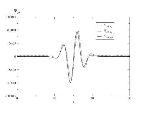
Figure 10: The numerically calculated waveforms (dashed and dotted curve) for the $\ell=2$, $m=0$ Teukolsky wave are compared with the analytic result (solid curve).

work, we also choose the Teukolsky wave with $m=0$. In prescribing the free function $F$ [cf. Eq. (6) in Teukolsky (1982)], we follow the suggestion by Eppley Eppley (1979) and superpose an ingoing and an outgoing wave packet. This packet is of Gaussian-like shape

$$F(x)=axe^{(-x/\sigma)^{2}},$$ (31)

with $x=t\mp r$. The resulting analytic expression for the Zerilli function $\Psi_{20}$ is rather lengthy but calculated straightforwardly. We evolve these data for $a=10^{-5}$ and $\sigma=1$ in octant symmetry on a numerical domain of size $20^{3}$ with two refinement levels, the fine level having half the extent and twice the resolution of the coarse. In Fig. 10 we compare the numerically computed $\Psi_{20}$ for resolutions $h_{1}=0.25$ (dashed) and $h_{2}=0.125$ (dotted curve) in the finer refinement level. We have also doubled the number of points on the extraction sphere from $80\times 40$ to $160\times 80$ in the $\theta$ and $\phi$ direction. In comparison the solid line represents the analytic result and demonstrates the convergence of the wave-forms. A quantitative evaluation shows that the convergence is fourth order in the early and late stages of this simulation and about third order in between when the wave pulse reaches the extraction radius $r_{\rm ex}=15$. This behavior is compatible with the fact that we use a fourth-order integration scheme for the integration on the sphere and the main evolution code is second-order convergent.

References

- Shibata et al. (2003) M. Shibata, K. Taniguchi, and K. Uryū, Phys. Rev. D 68, 084020 (2003), gr-qc/0310030.
- Marronetti et al. (2004) P. Marronetti, M. D. Duez, S. L. Shapiro, and T. Baumgarte, Phys. Rev. Lett. 92, 141101 (2004), gr-qc/0312036.
- Miller et al. (2004) M. Miller, P. Gressman, and W.-M. Suen, Phys. Rev. D 69, 064026 (2004), gr-qc/0312030.
- Brügmann et al. (2004) B. Brügmann, W. Tichy, and N. Jansen, Phys. Rev. Lett. 92, 211101 (2004), gr-qc/0312112.
- Miller (2005) M. Miller, Phys. Rev. D accepted (2005), gr-qc/0502087.
- Eppley (1975) K. R. Eppley, Ph.D. thesis, Princeton University (1975).
- Smarr et al. (1976) L. Smarr, A. Čadež, B. DeWitt, and K. Eppley, Phys. Rev. D 14, 2443 (1976).
- Smarr (1979) L. Smarr, in Sources of Gravitational Radiation, edited by L. Smarr (Cambridge University Press, Cambridge, 1979), pp. 245–274.
- Shibata and Nakamura (1995) M. Shibata and T. Nakamura, Phys. Rev. D 52, 5428 (1995).
- Friedrich (1996) H. Friedrich, Class. Quantum Gravit. 13, 1451 (1996).
- Frittelli and Reula (1996) S. Frittelli and O. A. Reula, Phys. Rev. Lett. 76, 4667 (1996), gr-qc/9605005.
- Anderson and York (1999) A. Anderson and J. W. York, Jr., Phys. Rev. Lett. 82, 4384 (1999), gr-qc/9901021.
- Baumgarte and Shapiro (1999) T. W. Baumgarte and S. L. Shapiro, Phys. Rev. D 59, 024007 (1999), gr-qc/9810065.
- Alcubierre et al. (2000) M. Alcubierre, G. Allen, B. Brügmann, E. Seidel, and W.-M. Suen, Phys. Rev. D 62, 124011 (2000), gr-qc/9908079.
- Kidder et al. (2001) L. E. Kidder, M. A. Scheel, and S. A. Teukolsky, Phys. Rev. D 64, 064017 (2001), gr-qc/0105031.
- Yoneda and Shinkai (2002) G. Yoneda and H.-A. Shinkai, Phys. Rev. D 66, 124003 (2002), gr-qc/0204002.
- Sarbach and Tiglio (2002) O. Sarbach and M. Tiglio, Phys. Rev. D 66, 064023 (2002), gr-qc/0205086.
- Bona et al. (2003) C. Bona, T. Ledvinka, C. Palenzuela, and M. Žáček, Phys. Rev. D 67, 104005 (2003), gr-qc/0302083.
- Alcubierre and Brügmann (2001) M. Alcubierre and B. Brügmann, Phys. Rev. D 63, 104006 (2001), gr-qc/0008067.
- Yo et al. (2002) H.-J. Yo, T. W. Baumgarte, and S. L. Shapiro, Phys. Rev. D 66, 084026 (2002), gr-qc/0209066.
- Alcubierre et al. (2003a) M. Alcubierre, B. Brügmann, P. Diener, M. Koppitz, D. Pollney, E. Seidel, and R. Takahashi, Phys. Rev. D 67, 084023 (2003a), gr-qc/0206072.
- Sperhake et al. (2004) U. Sperhake, K. L. Smith, B. Kelly, P. Laguna, and D. Shoemaker, Phys. Rev. D 69, 024012 (2004), gr-qc/0307015.
- Brandt et al. (2000) S. Brandt, R. Correll, R. Gómez, M. Huq, P. Laguna, L. Lehner, P. Maronetti, R. A. Matzner, D. Neilsen, J. Pullin, et al., Phys. Rev. Lett. 85, 5496 (2000), gr-qc/0009047.
- Alcubierre et al. (2004a) M. Alcubierre, B. Brügmann, P. Diener, F. Herrmann, D. Pollney, E. Seidel, and R. Takahashi (2004a), gr-qc/0411137.
- Alcubierre et al. (2004b) M. Alcubierre, B. Brügmann, P. Diener, F. S. Guzmán, I. Hawke, S. Hawley, F. Herrmann, M. Koppitz, D. Pollney, E. Seidel, et al. (2004b), AEI-2004-115, gr-qc/0411149.
- Anninos et al. (1993) P. Anninos, D. Hobill, E. Seidel, L. Smarr, and W.-M. Suen, Phys. Rev. Lett. 71, 2851 (1993), gr-qc/9309016.
- Anninos et al. (1995a) P. Anninos, D. Hobill, E. Seidel, L. Smarr, and W.-M. Suen, Phys. Rev. D 52, 2044 (1995a).
- Anninos et al. (1995b) P. Anninos, R. H. Price, J. Pullin, E. Seidel, and W.-M. Suen, Phys. Rev. D 52, 4462 (1995b), gr-qc/9505042.
- Baker et al. (1997) J. Baker, A. Abrahams, P. Anninos, S. Brandt, R. Price, J. Pullin, and E. Seidel, Phys. Rev. D 55, 829 (1997), gr-qc/9608064.
- Anninos and Brandt (1998) P. Anninos and S. Brandt, Phys. Rev. Lett. 81, 508 (1998), gr-qc/9806031.
- Price and Pullin (1994) R. H. Price and J. Pullin, Phys. Rev. Lett. 72, 3297 (1994), gr-qc/9402039.
- Abrahams and Cook (1994) A. M. Abrahams and G. B. Cook, Phys. Rev. D 50, R2364 (1994), gr-qc/9405051.
- Gleiser et al. (1996) R. J. Gleiser, C. O. Nicasio, R. H. Price, and J. Pullin, Phys. Rev. Lett. 77, 4483 (1996), gr-qc/9609022.
- Simone et al. (1995) L. E. Simone, E. Poisson, and C. M. Will, Phys. Rev. D 52, 4481 (1995), gr-qc/9506080.
- Baker et al. (2000) J. Baker, B. Brügmann, and M. Campanelli, Class. Quantum Grav. 17, L149 (2000), gr-qc/0003027.
- Brügmann (1999) B. Brügmann, Int. J. Mod. Phys. 8, 85 (1999), gr-qc/9708035.
- Alcubierre et al. (2001a) M. Alcubierre, W. Benger, B. Bügmann, G. Lanfermann, and L. Nerger, Phys. Rev. Lett. 87, 271103 (2001a), gr-qc/0012079.
- Fiske et al. (2005) D. R. Fiske, J. G. Baker, J. R. van Meter, D.-I. Choi, and J. M. Centrella (2005), gr-qc/0503100.
- Zlochower et al. (2005) Y. Zlochower, J. G. Baker, M. Campanelli, and C. O. Lousto (2005), gr-qc/0505055.
- Shoemaker et al. (2003) D. Shoemaker, K. Smith, U. Sperhake, P. Laguna, E. Schnetter, and D. Fiske, Class. Quantum Grav. 20, 3729 (2003), gr-qc/0301111.
- Schnetter et al. (2004) E. Schnetter, S. H. Hawley, and I. Hawke, Class. Quant. Grav. 21, 1465 (2004), gr-qc/0310042.
- Cook (2000) G. B. Cook, Living Rev. Relativity 2000-5 (2000), [Online Article] cited on 30 Sep 2004, http://relativity.livingreviews.org/Articles/lrr-2000-5.
- Matzner et al. (1998) R. A. Matzner, M. F. Huq, and D. Shoemaker, Phys. Rev. D 59, 024015 (1998), gr-qc/9805023.
- Marronetti et al. (2000) P. Marronetti, M. Huq, P. Laguna, L. Lehner, R. Matzner, and D. Shoemaker, Phys. Rev. D 62, 024017 (2000), gr-qc/0001077.
- Bonning et al. (2003) E. Bonning, P. Marronetti, D. Neilsen, and R. A. Matzner, Phys. Rev. D 68, 044019 (2003), gr-qc/0305071.
- York (1979) J. W. York, Jr., in Sources of Gravitational Radiation, edited by L. Smarr (Cambridge University Press, Cambridge, 1979), pp. 83–126.
- Bona et al. (1995) C. Bona, J. Massó, E. Seidel, and J. Stela, Phys. Rev. Lett. 75, 600 (1995), gr-qc/9412071.
- Alcubierre et al. (2001b) M. Alcubierre, B. Brügmann, D. Pollney, E. Seidel, and R. Takanashi, Phys. Rev. D 64, 061501 (2001b), AEI-2001-021, gr-qc/0104020.
- Alcubierre et al. (2003b) M. Alcubierre, A. Corichi, J. A. Gonzáles, D. Núñez, and M. Salgado (2003b), gr-qc/0303086.
- Alcubierre et al. (2003c) M. Alcubierre, A. Corichi, J. González, D. Núñez, and M. Salgado, Class. Quantum Grav. 20, 3951 (2003c), gr-qc/0303069.
- Gundlach and Martín-García (2004) C. Gundlach and J. M. Martín-García, Phys. Rev. D 70, 044032 (2004), gr-qc/0403019.
- Sarbach et al. (2002) O. Sarbach, G. Calabrese, J. Pullin, and M. Tiglio, Phys. Rev. D 66, 064002 (2002), gr-qc/0205064.
- Nagy et al. (2004) G. Nagy, O. E. Ortiz, and O. A. Reula, Phys. Rev. D 70, 044012 (2004).
- Baumgarte (2000) T. W. Baumgarte, Phys. Rev. D 62, 024018 (2000), gr-qc/0004050.
- Cook (1994) G. B. Cook, Phys. Rev. D 50, 5025 (1994), gr-qc/9404043.
- Thornburg (1996) J. Thornburg, Phys. Rev. D 54, 4899 (1996), gr-qc/9508014.
- Thornburg (2004) J. Thornburg, Class. Quantum Grav. 21, 743 (2004), gr-qc/0306056.
- Smarr (1975) L. Smarr, Ph.D. thesis, University of Texas at Austin (1975).
- Gunnarsen et al. (1995) L. Gunnarsen, H.-A. Shinkai, and K.-I. Maeda, Class. Quant. Grav. 12, 133 (1995), gr-qc/9406003.
- Kinnersley (1969) W. Kinnersley, J. Math. Phys. 10, 1195 (1969).
- Beetle et al. (2004) C. Beetle, M. Bruni, L. M. Burko, and A. Nerozzi (2004), gr-qc/0407012.
- Baker et al. (2002) J. Baker, M. Campanelli, and C. Lousto, Phys. Rev. D 65, 044001 (2002), gr-qc/0104063.
- Bishop et al. (1996) N. T. Bishop, R. Gómez, P. R. Holvorcem, R. A. Matzner, P. Papadopoulos, and J. Winicour, Phys. Rev. Lett. 76, 4303 (1996).
- d’Inverno and Vickers (1996) R. A. d’Inverno and J. A. Vickers, Phys. Rev. D 54, 4919 (1996).
- Winicour (2001) J. Winicour, Living Rev. Relativity 2001-3 (2001), [Article in Online Journal] cited on 23 Feb 2001, http://www.livingreviews.org/Articles/Volume4/2001-3winicour.
- Abrahams et al. (1998) A. M. Abrahams, L. Rezzolla, M. E. Rupright, A. Anderson, P. Anninos, T. W. Baumgarte, N. T. Bishop, S. R. Brandt, J. C. Browne, K. Camarda, et al., Phys. Rev. Lett. 80, 1812 (1998).
- Frittelli and Gómez (2004) S. Frittelli and R. Gómez, Phys. Rev. D 69, 124020 (2004), gr-qc/0404070.
- Beyer and Sarbach (2004) H. Beyer and O. Sarbach, Phys. Rev. D 70, 104004 (2004), gr-qc/0406003.
- Chandrasekhar and Detweiler (1975) S. Chandrasekhar and S. Detweiler, Proc. R. Soc. Lond. A. 344, 441 (1975).
- Cunningham et al. (1980) C. T. Cunningham, R. H. Price, and V. Moncrief, ApJ 236, 674 (1980).
- Moncrief (1974) V. Moncrief, Ann. Phys. 88, 323 (1974).
- Abrahams and Evans (1990) A. M. Abrahams and C. R. Evans, Phys. Rev. D 42, 2585 (1990).
- Abrahams et al. (1992) A. Abrahams, D. Bernstein, D. Hobill, E. Seidel, and L. Smarr, Phys. Rev. D 45, 3544 (1992).
- Camarda and Seidel (1999) K. Camarda and E. Seidel, Phys. Rev. D 59, 064019 (1999), gr-qc/9805099.
- Font et al. (2002) J. A. Font, T. Goodale, S. Iyer, M. Miller, L. Rezzolla, E. Seidel, N. Stergioulas, W.-M. Suen, and M. Tobias, Phys. Rev. D 65, 084024 (2002), gr-qc/0110047.
- Regge and Wheeler (1957) T. Regge and J. A. Wheeler, Phys. Rev. 108, 1063 (1957).
- Sarbach and Tiglio (2001) O. Sarbach and M. Tiglio, Phys. Rev. D 64, 084016 (2001).
- Gerlach and Sengupta (1978) U. H. Gerlach and U. K. Sengupta, Phys. Rev. D 19, 2268 (1978).
- Nagar and Rezzolla (2005) A. Nagar and L. Rezzolla (2005), gr-qc/0502064.
- Teukolsky (1982) S. A. Teukolsky, Phys. Rev. D 26, 745 (1982).
- Eppley (1979) K. Eppley, in Sources of Gravitational Radiation, edited by L. L. Smarr (Cambridge University Press, Cambridge, 1979), pp. 275–291.