On the Twin Paradox in a Universe with a Compact Dimension

Abstract

We consider the twin paradox of special relativity in a universe with a compact spatial dimension. Such topology allows two twin observers to remain inertial yet meet periodically. The paradox is resolved by considering the relationship of each twin to a preferred inertial reference frame which exists in such a universe because global Lorentz invariance is broken. The twins can perform “global” experiments to determine their velocities with respect to the preferred reference frame (by sending light signals around the cylinder, for instance). Here we discuss the possibility of doing so with local experiments. Since one spatial dimension is compact, the electrostatic field of a point charge deviates from $1/r^{2}$. We show that although the functional form of the force law is the same for all inertial observers, as required by local Lorentz invariance, the deviation from $1/r^{2}$ is observer-dependent. In particular, the preferred observer measures the largest field strength for fixed distance from the charge.

1 Introduction

In the classic presentation of the twin paradox, [1], two observers each witness the other receding at constant velocity and returning at the same velocity at a later time. Each observer will claim he was stationary and, by time dilation, that the other should be younger upon meeting. The resolution is that one observer turned around at some point during the journey and, consequently, was not inertial for the entire duration of the trip. This kinematic asymmetry allows both twins to unambiguously determine which of them aged more during the journey: the twin who remained inertial throughout.

In a space-time with one spatial dimension compactified, $S^{1}\times\mathbb{R}^{2,1}$, this kinematic solution no longer works. Both twins can remain inertial for the entire journey if they confine their motion to the compact dimension (see Fig. 1). In this case, the resolution lies in recognizing that compactifying a spatial dimension breaks global Lorentz invariance, [2]. In particular, there is now a preferred inertial reference frame, [2, 3, 4], namely that for which the circle is purely spatial (i.e., the observer whose worldline does not wind around the circle, [5]). The relationship of each observer to this reference frame establishes the asymmetry required to resolve the paradox: the observer in the preferred frame is essentially at rest with respect to the universe and ages more than the moving observer during the journey.

It is well known that observers can determine whether or not they are in the preferred rest frame by sending light beams in opposite directions along the compact dimension, [2, 4]. After waiting for the light beams to traverse the entire compact dimension, only the observer in the preferred frame will receive both signals simultaneously. Moreover, the time interval between the two signals is related to the velocity of the observer relative to the preferred frame.

Such a global experiment is of little practical use if the size of the circle is on the order of cosmological scales since an observer would have to wait about a Hubble time before receiving his signals. Here we present a local experiment that either twin can perform to determine his relationship to the preferred frame based on measuring deviations from the $1/r^{2}$ force law. The electric (or gravitational) field in a universe with a compact dimension is not exactly $1/r^{2}$ but depends on the size $L$ of the compact dimension because field lines are confined in this direction. Since local Lorentz invariance still holds, the functional form of the field is the same for all inertial observers, but the parameters which appear in the force law, which can be thought of as effective fine-structure (or Newton’s) constants, do depend on the observer. This can be understood qualitatively because the size of the compact dimension is not invariant under boosts. A boosted observer sees a larger effective circle (segment, actually) and thus a weaker field. Conversely, an observer in the preferred frame measures the strongest field at fixed distance from the source. Hence by making measurements of the electric field of a point charge stationary in their frame, observers may determine the effective length of the compact dimension in their frame, $L_{eff}$. Comparing $L_{eff}$ with $L$, the length of the compact dimension in the preferred frame, precisely specifies the relationship of the observer to the preferred frame and resolves the paradox: the boosted observer ages less during the paradox by a factor $\gamma=L_{eff}/L$.

2 Analysis of the Paradox and a Global Resolution

2.1 Description of the Space-time

The manifold we are considering in this problem is the cylinder, $S^{1}\times\mathbb{R}^{2,1}$, with the Minkowski metric, $ds^{2}=-dt^{2}+dx^{2}+dy^{2}+dz^{2}$. It can be constructed from $\mathbb{R}^{2,1}$ by imposing the equivalence relation

$$(t,x,y,z)\sim(t,x+nL,y,z)$$ (1)

where $L$ is the circumference of the compact dimension and $n$ is an integer. Each equivalence class of points $\left[(t,x+nL,y,z)\right]$ in $\mathbb{R}^{3,1}$ is represented by a single point $(t,x,y,z)$ on the cylinder, chosen such that $0\leq x<L$.

We thus have two equivalent pictures of the manifold $S^{1}\times\mathbb{R}^{2,1}$: the “wrapped” picture, Fig. 1, where each point is a unique event, and the “unwrapped” picture in the covering space, Fig. 1, where an infinity of points represents the same event. We can consider the latter picture as an infinite sheet of paper which we “wrap” into a cylinder to construct the former picture. It will prove useful to be able to switch back and forth between these two pictures.

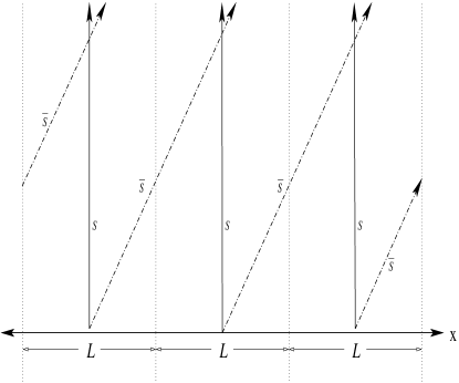
Figure 1: The worldlines of the preferred observer ($S$) and the non-preferred observer ($\overline{S}$) in the wrapped picture (a) and the unwrapped picture (b).

Lorentz invariance is broken globally since one dimension is compact, which leads to the existence of a preferred rest frame. To see this, consider that the equivalence relation (1) is manifestly dependent on coordinates and so is itself defined in a particular frame, call it $S$. In this frame, a point $p=(t_{0},x_{0},y_{0},z_{0})$ in the wrapped picture corresponds to an infinity of points $p_{n}=(t_{0},x_{0}+nL,y_{0},z_{0})$ in the unwrapped picture. These points are all simultaneous in $S$ and they differ from each other only by spatial translations. What about $\overline{S}$, a frame moving with respect to $S$ at some velocity $\beta=v/c$? In this frame, the point $p$ has coordinates $p=(\overline{t_{0}},\overline{x_{0}},\overline{y_{0}},\overline{z_{0}})=(\gamma t_{0}-\beta\gamma x_{0},\gamma x_{0}-\beta\gamma t_{0},y_{0},z_{0})$, where $\gamma=(1-\beta^{2})^{1/2}$. In the unwrapped picture, this point corresponds to the points $p_{n}=(\gamma t_{0}-\beta\gamma x_{0}-\beta\gamma nL,\gamma x_{0}+\gamma nL-\beta\gamma t_{0},y_{0},z_{0})=(\overline{t_{0}}-\beta\gamma nL,\overline{x_{0}}+\gamma nL,y_{0},z_{0})$. We see that the equivalence relation (1) in an arbitrary inertial frame $\overline{S}$ becomes

$$(\overline{t},\overline{x},\overline{y},\overline{z})\sim(\overline{t}-n\beta\gamma L,\overline{x}+n\gamma L,\overline{y},\overline{z})$$ (2)

Thus, the image points simultaneous in frame $\overline{S}$ are not only translated through space, but through time as well. This is a recognition of the fact that lines of equal time for observers with $\beta\neq 0$ do not close on themselves but spiral around the cylinder. There is only one observer, characterized by $\beta=0$, whose line of equal time closes on itself, and for whom the identification (2) is a purely spatial one. We refer to the frame of this observer as the preferred rest frame.

It should be noted that the effective size of the compact dimension in a frame $\overline{S}$ is $\gamma L$, as can be seen directly from (2). We thus define the effective length of the compact dimension:

$$L_{eff}\equiv\gamma L$$ (3)

The preferred observer measures the smallest value of $L_{eff}$, namely $L$.

2.2 Minkowski Diagrams and Transition Functions

The essential problem with the twin paradox in this space-time is that both twins can draw Minkowski diagrams which depict the other twin winding around the circle and coming back. Hence each twin will predict that the other is younger. We can resolve this contradiction by noting that, for the preferred observer, the images of the fundamental domain $(0,L)$ are simply translated spatially by (2). For a non-preferred observer, however, these images are also translated in time. This implies that a diagram like Fig.1 is not valid in a non-preferred frame, and that a non-preferred observer cannot naively draw Minkowski diagrams. Instead, the non-preferred observer must take into account certain transition functions.

Because one dimension is compact, observers in our space-time have a problem with multi-valued coordinates. In Sec. 2.1 we glossed over this point and implicitly treated all lengths in the $x$-dimension modulo $L$. To be more precise, we should really cover the manifold $S^{1}\times\mathbb{R}^{2,1}$ with two single-valued coordinate patches and glue them together with appropriate transition functions.

In some coordinate system $S$, let patch $A$ cover the entirety of the $t$, $y$, and $z$ dimensions and cover an open interval $(0,L_{eff})$ of the compact $x$-dimension. Likewise, let patch $B$ cover the entirety of the uncompact dimensions and cover an interval $(-\epsilon,\epsilon)$ in the $x$-dimension. As an analogy, one may think of patch $A$ as a piece of paper wrapped around the cylinder and patch $B$ as a strip of tape applied on the seam of patch $A$.

Figure 2: We require two patches, $A$ and $B$, to cover the manifold $S^{1}\times\mathbb{R}^{2,1}$

As we pass from patch $A$ to patch $B$, we wind around the cylinder or, equivalently, move to another image patch in the unwrapped picture, Fig. 1. The index $n$ can thus be thought of as winding number, [5]. If observers keep track of the winding number of light signals, etc., Eq. (2) describes how to relabel paths as their winding number changes. Since a change in winding number corresponds to leaving patch $A$, crossing through patch $B$, and returning to patch $A$, Eq. (2) is recognized to be exactly the transition function we need:

$$f_{\pm}(t,x,y,z)=(t\pm\beta\gamma L,x\mp\gamma L,y,z)\,,$$ (4)

where $f_{+}$ and $f_{-}$ are the transition functions used when winding around in the positive and negative $x$-directions, respectively.

When a given observer attempts to describe the physics within a single patch, say patch $A$, he must keep track of how to adjust the coordinates he assigns to objects as they exit and then re-enter the patch. For observer $S$, in the preferred frame, $\beta=0$, and there is no translation in time as objects wind around the universe. This is why he can naively draw diagrams like Fig. 1. For observer $\overline{S}$, however, $\beta\neq 0$, and the transition functions involve translations in time. In this frame, a diagram like Fig. 1 would simply be incorrect. Figure 3 properly depicts the situation in both frames using the appropriate transition functions. No contradiction ensues.

Figure 3: Minkowski diagrams depicting the twin paradox from the preferred frame (a) and a non-preferred frame moving with $\beta=0.5$ (b). The thick lines represent the worldlines of the twins and the dotted lines, labeled by $+$ and $-$, represent two light signals which wrap around the circle in the positive and negative $x$-directions, respectively. Note that the preferred observer ($S$) receives both $+$ and $-$ light signals at the same point ($P$) while the non-preferred observer ($\overline{S}$) receives them at two different points ($P_{+}$ and $P_{-}$).

If both twins know their velocity with respect to the preferred frame, then, by Eq. (4), they can find their transition functions and use them to draw correct diagrams. By using the transition functions, both observers in the twin paradox come to the conclusion that the twin in the non-preferred frame ages less during the journey by a factor of $\gamma$.

2.3 Einstein Synchronization on the Cylinder

We have thus far used two coordinate patches for the purely mathematical reason of avoiding multi-valued coordinates. The need for multiple patches can, of course, be understood from a physical point of view by considering the synchronization of clocks in this space-time.

The usual method for synchronizing clocks is Einstein synchronization: if an observer is midway between two clocks and receives light signals from each clock with the same reading simultaneously then the two clocks are said to be Einstein synchronized. Usually, Einstein synchronization is a transitive process: if clock $A$ is synchronized with clock $B$, and clock $B$ is synchronized with clock $C$, then clock $A$ is synchronized with clock $C$.

Einstein synchronization immediately fails on a compact dimension because there are two midpoints between any pair of clocks. We can circumvent this problem by choosing a “left-most” and a “right-most” clock. These clocks will demarcate the edges of what will become a coordinate patch. We can synchronize clocks by using the midpoint in between these two boundary clocks, the midpoint in the coordinate patch we are constructing. Transitivity is preserved because we confine all our procedures to this single patch which, without global data, is indistinguishable from an uncompact space.

A problem occurs when we let the left-most and right-most clocks approach each other, letting our coordinate patch encircle the entire compact dimension. As soon as they overlap, that is, as soon as the left-most clock and the right-most clock are the same clock, we will have constructed a global rest frame and, in a non-preferred frame, this clock will have to read one time to be synchronized with the clock on its left and another time to be synchronized with the clock on its right. This is easily seen by considering lines of equal time in the wrapped picture. For the preferred observer, such lines close on themselves and form circles. For a non-preferred observer, however, they do not close but instead spiral endlessly around the cylinder. The non-preferred observer’s coordinate system corresponds to a segment of such a spiral. If this is to span the cylinder, then the segment of the spiral must also span the cylinder. However, if we require each clock to only read one time, this implies that it must be discontinuous at a point. The transition functions (4) are a reflection of this fact. Therefore, while it is possible for the boosted observer to synchronize clocks in this way, evidently this comes at the expense of homogeneity. Indeed, it introduces a special line on the cylinder where time jumps.

In fact, there is a perspicuous analogy between the use of transition functions and patches on this space-time and a more familiar phenomenon: the time zones on the Earth. Imagine a person standing on the equator keeping time by the Sun. In his reference frame, fixed at a point on the Earth’s surface, the Sun revolves about the Earth once per day. He attempts to label points on the equator with their distance from him and with a particular time based on the position of the Sun as seen from that point. At a particular moment, let him declare that it is high noon at his own position. Points on the equator east of him will be assigned later times, while points west will be assigned earlier times. As long as his reference frame is local and doesn’t span the equator, nothing goes wrong in his scheme. As soon as it does, however, the point diametrically opposite him on the equator demands to be labeled by two points in time, one to coincide with the points immediately east of it and another for the points immediately west. His solution is to draw an international date line through that point – a transition function or discontinuity in his coordinate system.

2.4 Global Experiment to Distinguish Twin Observers

To determine his velocity with respect to the preferred frame, an observer can send out light signals in opposite directions along the compact $x$-dimension, [2]. From Fig. 3 it is clear that the preferred observer, whose transition function does not involve translations in time, will receive the signals at the same time (at the event labeled by $P$). A non-preferred observer, however, will measure a time-delay in the reception of the two signals (the events $P_{+}$ and $P_{-}$). A simple calculation yields

$$\beta=\frac{\tau(P_{+})-\tau(P_{-})}{\tau(P_{+})+\tau(P_{-})}\,,$$ (5)

where $\tau(P)$ is the proper time at which event $P$ occurs. This expression can be used to determine the velocity with respect to the preferred frame. For the preferred observer, one has $\beta=0$ and indeed $\tau(P_{+})=\tau(P_{-})$. Once an observer knows his velocity with respect to the preferred frame, he can easily calculate the transition functions (4) and draw appropriate Minkowski diagrams.

3 Electromagnetism and a Local Resolution

The experiment described above would take a prohibitively long time in a universe of any realistic size, as light signals have to encircle the entire compact dimension! Furthermore, this global solution does not seem as satisfying as the local solution to the twin paradox in standard space-time $\mathbb{R}^{3,1}$. In the standard space-time, each observer may easily conduct local experiments to determine whether or not he is the accelerated twin – he could hang a pendulum, for example, and watch for any deviations in its path during the journey.

It seems that any local kinematic experiment would not serve to resolve the paradox because there are no local kinematic differences between the two observers which might be exploited to distinguish them. The global solution already presented works precisely because it is global - the light beams traverse the entire compact dimension, cross between coordinate patches, and thus force the observers to use transition functions, which encode the relationship between the observer and the preferred rest frame. Here we propose to exploit the local consequences of global phenomena such as electric or gravitational fields. A field permeates all of space and thus “knows” about the global topology. This global knowledge can be extracted by making measurements of the field at a few points.

3.1 Electromagnetism on $S^{1}\times\mathbb{R}^{2,1}$

Consider the electromagnetic field of a point charge $q$ at rest at the origin of the preferred rest frame. One expects that the formula for the electromagnetic field of this point charge should deviate from the usual $1/r^{2}$ since the field lines cannot spread as much in the compact direction. Moreover, such deviations should depend on the size of the circle, $L$.

Figure 4: A single image charge stationary at the origin of the preferred frame may be considered as an infinite number of image charges in the unwrapped picture (a). A charge moving at constant velocity in the preferred frame (b) may be considered as a charge stationary at the origin of a boosted, non-preferred frame. In this frame, we may again consider the single charge as an infinite number of image charges (c).

To calculate the field, it is easiest to work in the unwrapped picture and consider each image charge as a source for the electromagnetic field at the field point (see Fig. 4). There is no magnetic field, of course, since the point charge and hence all its image charges are at rest in this frame. We find

$$\vec{E}_{S}(x,y,z)=\frac{q}{4\pi\epsilon_{0}}\sum_{n=-\infty}^{\infty}\frac{(x+nL)\hat{x}+y\hat{y}+z\hat{z}}{\left[(x+nL)^{2}+y^{2}+z^{2}\right]^{\frac{3}{2}}}\,,$$ (6)

which depends on $L$, as expected. It is easy to see that one recovers the usual Coulomb law in the limit $L\to\infty$.

What about the electric field of a point charge stationary in a non-preferred frame? Because Lorentz invariance is locally valid in this space-time, the field measured by a non-preferred observer should have the same functional form as Eq. (6) – it can only differ in the values of some parameters. The only parameter to be found in Eq. (6) is the length of the compact dimension, $L$. Thus we expect $L$ to be replaced with $L_{eff}$, the effective length of the compact dimension as measured by an observer in a non-preferred frame.

This answer is most easily obtained by noting that a point charge stationary in a non-preferred frame is of course moving at some constant velocity with respect to the preferred observer. From the preferred frame, we can boost directly into the rest frame of the charge and find that we have reproduced the situation we started with prior to deriving Eq. (6): a stationary point charge and an infinite series of image charges, each separated by the effective length of the compact dimension in that frame, $L_{eff}$. This is illustrated in Fig. 4. Thus, we have

$$\vec{E}_{\overline{S}}(x,y,z)=\frac{q}{4\pi\epsilon_{0}}\sum_{n=-\infty}^{\infty}\frac{(x+nL_{eff})\hat{x}+y\hat{y}+z\hat{z}}{\left[(x+nL_{eff})^{2}+y^{2}+z^{2}\right]^{\frac{3}{2}}}$$ (7)

for an arbitrary frame $\overline{S}$. The only change from Eq. (6) is a substitution $L\to L_{eff}$. The field measured by any observer in this universe thus has a dependence on the parameter $L_{eff}$, the effective length of the universe in the frame of the observer.

A local experiment immediately suggests itself. If we presume observers in this space-time know the value of $L$, then measuring the electric field of a stationary point charge at a few points is enough to determine $L_{eff}$, from which one can determine $\beta$ and resolve the twin paradox.

Restricting our attention to points on the $x$-axis, the infinite sum in Eq. (7) can be written in closed form using residue theorems and then expanded in powers of $x/L^{2}$:

$$\vec{E}_{\overline{S}}(x,0,0) = \frac{q}{4\pi\epsilon_{0}}\sum_{n=-\infty}^{\infty}\frac{\hat{x}}{(x+nL_{eff})^{2}}$$ (8)

$$= \frac{q}{4\pi\epsilon_{0}}\frac{\pi^{2}}{L_{eff}^{2}}\csc^{2}\left(\frac{\pi x}{L_{eff}}\right)\hat{x}$$

$$= \frac{q}{4\pi\epsilon_{0}}\left[\frac{1}{x^{2}}+\frac{\pi^{2}}{3L_{eff}^{2}}+\mathcal{O}\left(\frac{x^{2}}{L_{eff}^{4}}\right)\right]\hat{x}\,.$$

It is intriguing to note that the first order correction to the electric field (along the $x$-axis) in this topology is constant, with the fractional difference from the usual Coulomb field given by

$$\frac{\Delta E}{E}\approx\frac{\pi^{2}}{3}\left(\frac{x}{L}\right)^{2}.$$ (9)

As expected, the difference increases with decreasing $L$.

If this experiment is to be practical, however, then the ratio $\Delta E/E$ must not be vanishingly small. The smallest allowed $L$ is $L=24$ Gpc from cosmic microwave background analysis, [7] (though this figure may require revision, see, [8]). Unfortunately, for any realistic $x$, this ratio is unmeasurably small. Moreover, it is easily seen that the difference in magnitude between the fields measured in the preferred frame and a non-preferred frame is further suppressed by a factor of $\beta^{2}$ in the non-relativistic limit.

There are two points to be made about the above derivation. First of all, Eq. (8) assumes that the charge has been at rest for sufficiently long so that our expression for the electrostatic field applies. The analysis of a moving charge would require taking into account the self-interactions with radiated photons that circle around the compact dimension and hit the charge back. Secondly, we have completely neglected cosmic expansion and approximated our universe as static. Modeling the paradox on an expanding cylinder (or any compact Friedmann-Robertson-Walker universe) introduces many subtleties, [9, 10].

4 Acknowledgements

The authors would like to thank Justin Khoury for his supervision during this work. We would also like to thank Allan Blaer, Brian Greene, Dan Kabat, Janna Levin, Maulik Parikh, and Amanda Weltman for helpful discussions. This work was supported by the VIGRE program of the Columbia University Departments of Mathematics and Physics.

References

- [1] E.F. Taylor and J.A. Wheeler, Spacetime Physics, New York, 1963.
- [2] C.H. Brans and D.R. Stewart, Phys. Rev. D8, 1662 (1973).
- [3] J.D. Barrow and J. Levin, gr-qc/0101014.
- [4] P.C. Peters, Am. J. Phys. 51, 791 (1983).
- [5] J.P. Uzan, R. Lehoucq, J.P. Luminet and P. Peter, Eur. J. Phys. 23, 277 (2002).
- [6] C.L. Bennett et al., Ap.J. Suppl, 148, 1 (2003).
- [7] N.J. Cornish, D.N. Spergel, G.D. Starkman, and E. Komatsu, astro-ph/0310233.
- [8] J. Levin, astro-ph/0403036.
- [9] J. Levin and M.K. Parikh, private communication.
- [10] P.C. Peters, Am. J. Phys. 54, 334 (1986).