Braneworld Cosmology

Abstract

We present a general formalism for studying an inflationary scenario in the two-brane system. We explain the gradient expansion method and obtain the 4-dimensional effective action. Based on this effective action, we give a basic equations for the background homogeneous universe and the cosmological perturbations. As an application, we propose a born-again braneworld scenario.

Keywords: cosmology, low-energy, gradient expansion, born-again-braneworld

1 Introduction

It is widely believed that the initial singularity problem in the conventional standard cosmology can be resolved by the quantum theory of gravity. It is also known that the most promising candidate for the quantum theory of gravity is the superstring theory. Remarkably, the superstring theory precisely predicts the existence of extra-dimensions. As our universe can be recognized as the 4-dimensional Lorentzian manifold by experience, the necessity for reconciling the prediction of the superstring theory with our experience is apparent.

The solution to this problem was proposed by Kaluza and Klein a long time ago. Their idea is simply that the extra-dimensions are too tiny to see them. In fact, in order to fit our real world, the sizes of the internal dimensions are constrained to be the Planck length. This beautiful answer has been considered to be a unique one for a long time. However, the recent discovery of Dp-brane solutions has changed the situation. The Dp-brane is a kind of soliton solution with the p-dimensional spatial and 1-dimensional temporal extension on which the boundary of open strings can be attached. While closed strings can freely propagate in the whole 10-dimensional spacetime. Since the open string contains the standard matter and the closed string contains the graviton, the D-brane solution yields the idea of the braneworld where the standard matters are confined to the 4-dimensional braneworld, while the gravitons can propagate in the 10-dimensional bulk spacetime. Interestingly, in the case of the braneworld, the constraint on the sizes of the internal dimensions is not so stringent compared with the case of Kaluza-Klein mechanism. Indeed, the accelerator experiments in the laboratory can not give the strong constraints because the standard matters are confined to the 4-dimensional braneworld. Moreover, the experiment of the Newtonian force is rather poor at scales smaller than 0.1 mm. Hence, the sizes of the extra-dimensions could be 0.1 mm in this braneworld picture.

Because of the possibility of the large extra-dimensions in the braneworld models, the early universe must be studied with careful considerations of the effects of the bulk geometry. In this sense, the extra-dimensions can be regarded as the new elements of the universe.

To be more precise, what we want to explore is the effects of the bulk geometry on the generation and the evolution of the cosmological fluctuations. In the conventional 4-dimensional cosmological models, curvature fluctuations with the flat spectrum are generated from the quantum fluctuations during the inflationary expansion. Then, its amplitude is freezed till the wavelength crosses the horizon again. Now, this curvature fluctuations can be observed through the cosmic microwave background radiation. There are various possible sources to alter this standard scenario in the braneworld models. The most obvious possibility is the collision between different braneworlds. In related to this case, there may be the effect of the radion, namely the distance between two braneworlds. Moreover, there are effects due to gravitational waves propagating in the bulk, this is often called as Kaluza-Klein (KK) effects.

There are many braneworld models. As a representative, here we will concentrate on the simplest Randall-Sundrum two-brane model [1]. In this paper, using the gradient expansion method, we formulate the general scheme to investigate effects of the bulk geometry. As an application, we propose the born-again braneworld scenario and discuss its resemblance to the pre-big-bang model [2]. We also make observational predictions on the spectrum of the primordial gravitational waves which turns out to be very blue.

2 Inflation on braneworld

Let us start with the effective Friedmann equation

$$H^{2}={\kappa^{4}\mu^{2}\over 12}-{3\over\ell^{2}}+{\kappa^{2}\over\ell}\rho+\kappa^{4}\rho^{2}+{{\cal C}\over\alpha^{4}}\ ,$$ (1)

where $H$, $\alpha$ and $\rho$ are, respectively, the Hubble parameter, the scale factor and the total energy density of each brane. The Newton’s constant can be identified as $8\pi G_{N}=\kappa^{2}/\ell$. Here, ${\cal C}$ is a constant of integration associated with the mass of a black hole in the bulk. This constant ${\cal C}$ is referred to as the dark radiation in which the effect of the bulk is encoded. The effective cosmological constant for the braneworld becomes

$$\Lambda_{\rm eff}={\kappa^{4}\mu^{2}\over 12}-{3\over\ell^{2}}\ ,$$ (2)

where $\mu$ and $\ell$ are the tension of the brane and the curvature scale in the bulk which is determined by the bulk vacuum energy, respectively. For $\kappa^{2}\mu=6/\ell$, we have Minkowski spacetime as a solution. In order to obtain the inflationary universe, we need the positive effective cosmological constant. In the brane world model, there are two possibilities. One is to increase the brane tension and the other is to increase $\ell$. The brane tension can be controled by the scalar field on the brane. The bulk curvature scale $\ell$ can be controled by the bulk scalar field. The former case is a natural extension of the 4-dimensional inflationary scenario [3]. The latter possibility is a novel one peculiar to the brane model. Recall that, in the superstring theory, scalar fields are ubiquitous. Indeed, the dilaton and moduli exists in the bulk generically, because they arise as the modes associated with the closed string. Moreover, when the supersymmetry is spontaneously broken, they may have the non-trivial potential. Hence, it is natural to consider the inflationary scenario driven by these fields [4]. Now, we develop the formalism to investigate these inflating braneworlds.

3 Gradient Expansion Method

In this section, for simplicity, we explain the gradient expansion method using the single-brane model. We use the Gaussian normal coordinate system

$$ds^{2}=dy^{2}+g_{\mu\nu}(y,x)dx^{\mu}dx^{\nu}$$ (3)

to describe the geometry of the brane world. Note that the brane is located at $y=0$ in this coordinate system. Decomposing the extrinsic curvature $K_{\mu\nu}=-g_{\mu\nu,y}/2$ into the traceless and the trace part $K_{\mu\nu}=\Sigma_{\mu\nu}+{1\over 4}g_{\mu\nu}K\ ,$ we obtain the basic equations which hold in the bulk;

$$\Sigma^{\mu}{}_{\nu,y}-K\Sigma^{\mu}{}_{\nu}=-\left[\overset{(4)}{R}{}^{\mu}{}_{\nu}-{1\over 4}\delta^{\mu}_{\nu}\overset{(4)}{R}\right]\ ,$$ (4)

$${3\over 4}K^{2}-\Sigma^{\alpha}{}_{\beta}\Sigma^{\beta}{}_{\alpha}=\left[~{}\overset{(4)}{R}~{}\right]+{12\over\ell^{2}}\ ,$$ (5)

$$\nabla_{\lambda}\Sigma_{\mu}{}^{\lambda}-{3\over 4}\nabla_{\mu}K=0\ ,$$ (6)

where $\nabla_{\mu}$ denotes the covariant derivative with respect to the metric $g_{\mu\nu}$ and $\overset{(4)}{R}{}^{\mu}{}_{\nu}$ is the curvature associated with it. One also have the junction condition

$$\left[K^{\mu}{}_{\nu}-\delta^{\mu}_{\nu}K\right]\Big{|}_{y=0}={\kappa^{2}\over 2}\left(-\mu\delta^{\mu}_{\nu}+T^{\mu}{}_{\nu}\right)\ ,$$ (7)

where $T_{\mu\nu}$ is the energy momentum tensor of the matter. Recall that we are considering the $Z_{2}$ symmetric spacetime.

The problem now is separated into two parts. First, we will solve the bulk equations of motion with the Dirichlet boundary condition at the brane, $g_{\mu\nu}(y=0,x^{\mu})=h_{\mu\nu}(x^{\mu})$. After that, the junction condition will be imposed at the brane. As it is the condition for the induced metric $h_{\mu\nu}$, it is naturally interpreted as the effective equations of motion for gravity on the brane.

In this paper, we will consider the low energy regime in the sense that the energy density of matter, $\rho$, on the brane is smaller than the brane tension, ı.e., $\epsilon\equiv\rho/\mu\ll 1$. In this regime, we can use the gradient expansion method where the above ratio $\epsilon$ is the expansion parameter [5].

At zeroth order, we can neglect the curvature term. Anisotropic term must vanish in order to satisfy the junction condition. Now, it is easy to solve the remaining equations. The result is $\overset{(0)}{K}={4\over\ell}\ .$ Using the definition of the extrinsic curvature, we get the zeroth order metric as

$$ds^{2}=dy^{2}+a^{2}(y)h_{\mu\nu}(x^{\mu})dx^{\mu}dx^{\nu}\ ,\quad a(y)=e^{-2{y\over\ell}}\ ,$$ (8)

where the tensor $h_{\mu\nu}$ is the induced metric on the brane. From the zeroth order junction condition, we obtain the well known relation $\kappa^{2}\mu=6/\ell$. Hereafter, we will assume that this relation holds exactly.

The iteration scheme consists in writing the metric $g_{\mu\nu}$ as a sum of local tensors built out of the induced metric on the brane, the number of gradients increasing with the order. Hence, we will seek the metric as a perturbative series

$$g_{\mu\nu}(y,x^{\mu})=a^{2}(y)\left[h_{\mu\nu}(x^{\mu})+\overset{(1)}{g}{}_{\mu\nu}(y,x^{\mu})+\overset{(2)}{g}{}_{\mu\nu}(y,x^{\mu})+\cdots\right]\ ,$$ (9)

where $a^{2}(y)$ is extracted and we put the Dirichlet boundary condition $\overset{(i)}{g}{}_{\mu\nu}(y=0,x^{\mu})=0\ ,$ so that $g_{\mu\nu}(y=0,x)=h_{\mu\nu}(x)$ holds at the brane. Other quantities can be also expanded as

$$K^{\mu}{}_{\nu} = {1\over\ell}\delta^{\mu}_{\nu}+\overset{(1)}{K}{}^{\mu}{}_{\nu}+\overset{(2)}{K}{}^{\mu}{}_{\nu}+\cdots$$

$$\Sigma^{\mu}{}_{\nu} = \qquad+\overset{(1)}{\Sigma}{}^{\mu}{}_{\nu}+\overset{(2)}{\Sigma}{}^{\mu}{}_{\nu}+\cdots\ .$$ (10)

The next order solutions are obtained by taking into account the terms neglected at zeroth order. Substituting the zeroth order metric into $\overset{(4)}{R}(g)$, we obtain

$$\overset{(1)}{K}={\ell\over 6a^{2}}R(h)\ .$$ (11)

Hereafter, we omit the argument of the curvature for simplicity. Simple integration of Eq. (4) also gives the traceless part of the extrinsic curvature as

$$\overset{(1)}{\Sigma}{}^{\mu}{}_{\nu}={\ell\over 2a^{2}}(R^{\mu}{}_{\nu}-{1\over 4}\delta^{\mu}_{\nu}R)+{\chi^{\mu}{}_{\nu}(x)\over a^{4}}\ ,$$ (12)

where the homogeneous solution satisfies the constraints $\chi^{\mu}{}_{\mu}=0\ ,\ \chi^{\mu}{}_{\nu|\mu}=0\ .$ This term corresponds to dark radiation at this order.

At this order, the junction condition can be written as

$$\left[~{}\overset{(1)}{K}{}^{\mu}{}_{\nu}-\delta^{\mu}_{\nu}\overset{(1)}{K}~{}\right]\Bigg{|}_{y=0}={\ell\over 2}\left(R^{\mu}{}_{\nu}-{1\over 2}\delta^{\mu}_{\nu}R\right)+\chi^{\mu}{}_{\nu}={\kappa^{2}\over 2}T^{\mu}{}_{\nu}\ .$$ (13)

Thus, we have obtained the effective equation on the brane.

4 Effective Action for Two-brane System

We consider the two-brane system in this section. Without matter on the branes, we have the relation between the induced metrics, $g^{\ominus\hbox{-}\rm brane}_{\mu\nu}=e^{-2d/\ell}g^{\oplus\hbox{-}\rm brane}\equiv\Omega^{2}g^{\oplus\hbox{-}\rm brane}$ where $d$ is the distance between the two branes. Here, $\oplus$ and $\ominus$ represent the positive and the negative tension branes, respectively. Although $\Omega$ is constant for vacuum branes, it becomes the function of the 4-dimensional coordinates if we put the matter on the brane.

Adding the energy momentum tensor to each of the two branes, and allowing deviations from the pure AdS₅ bulk, the effective (non-local) Einstein equations on the branes at low energies take the form [6],

$$G^{\mu}{}_{\nu}(h) = {\kappa^{2}\over\ell}\overset{\oplus}{T}{}^{\mu}{}_{\nu}-{2\over\ell}\chi^{\mu}{}_{\nu}\,,$$ (14)

$$G^{\mu}{}_{\nu}(f) = -{\kappa^{2}\over\ell}\overset{\ominus}{T}{}^{\mu}{}_{\nu}-{2\over\ell}{\chi^{\mu}{}_{\nu}\over\Omega^{4}}\ .$$ (15)

where $h_{\mu\nu}=g^{\oplus\hbox{-}{\rm brane}}_{\mu\nu}$, $f_{\mu\nu}=g^{\ominus\hbox{-}{\rm brane}}_{\mu\nu}=\Omega^{2}h_{\mu\nu}$ and the terms proportional to $\chi_{\mu\nu}$ are 5-dimensional Weyl tensor contributions which describe the non-local 5-dimensional effect. Although Eqs. (14) and (15) are non-local individually, with undetermined $\chi_{\mu\nu}$, one can combine both equations to reduce them to local equations for each brane. Since $\chi_{\mu\nu}$ appears only algebraically, one can easily eliminate $\chi_{\mu\nu}$ from Eqs. (14) and (15). Defining a new field $\Psi=1-\Omega^{2}$, we find

$$G^{\mu}{}_{\nu}(h) = {\kappa^{2}\over\ell\Psi}\overset{\oplus}{T}{}^{\mu}{}_{\nu}+{\kappa^{2}(1-\Psi)^{2}\over\ell\Psi}\overset{\ominus}{T}{}^{\mu}{}_{\nu}$$ (16)

$$+{1\over\Psi}\left(\Psi^{|\mu}{}_{|\nu}-\delta^{\mu}_{\nu}\Psi^{|\alpha}{}_{|\alpha}\right)+{3\over 2\Psi(1-\Psi)}\left(\Psi^{|\mu}\Psi_{|\nu}-{1\over 2}\delta^{\mu}_{\nu}\Psi^{|\alpha}\Psi_{|\alpha}\right)\ ,$$

where $|$ denotes the covariant derivative with respect to the metric $h_{\mu\nu}$. Since $\Omega$ (or equivalently $\Psi$) contains the information of the distance between the two branes, we call $\Omega$ (or $\Psi$) the radion. We can also determine $\chi^{\mu}{}_{\nu}$ by eliminating $G^{\mu}{}_{\nu}$ from Eqs. (14) and (15). Then,

$$\chi^{\mu}{}_{\nu} = -{\kappa^{2}(1-\Psi)\over 2\Psi}\left(\overset{\oplus}{T}{}^{\mu}{}_{\nu}+(1-\Psi)\overset{\ominus}{T}{}^{\mu}{}_{\nu}\right)$$ (17)

$$-{\ell\over 2\Psi}\left[\left(\Psi^{|\mu}{}_{|\nu}-\delta^{\mu}_{\nu}\Psi^{|\alpha}{}_{|\alpha}\right)+{3\over 2(1-\Psi)}\left(\Psi^{|\mu}\Psi_{|\nu}-{1\over 2}\delta^{\mu}_{\nu}\Psi^{|\alpha}\Psi_{|\alpha}\right)\right]\ .$$

Note that the index of $\overset{\ominus}{T}{}^{\mu}{}_{\nu}$ is to be raised or lowered by the induced metric on the $\ominus$-brane, $f_{\mu\nu}$. The condition $\chi^{\mu}{}_{\mu}=0$ yields

$$\Box\Psi = {\kappa^{2}\over 3\ell}(1-\Psi)\left\{\overset{\oplus}{T}+(1-\Psi)\overset{\ominus}{T}\right\}-{1\over 2(1-\Psi)}\Psi^{|\mu}\Psi_{|\mu}\ .$$ (18)

The effective action for the $\oplus$-brane which gives Eqs. (16) and (18) is

$$S_{\oplus} = {\ell\over 2\kappa^{2}}\int d^{4}x\sqrt{-h}\left[\Psi R-{3\over 2(1-\Psi)}\Psi^{|\alpha}\Psi_{|\alpha}\right]$$ (19)

$$\!\!\!\!\!\!\!\!\!\!+\int d^{4}x\sqrt{-h}{\cal L}^{\oplus}+\int d^{4}x\sqrt{-h}\left(1-\Psi\right)^{2}{\cal L}^{\ominus}\ .$$

We now extend the analysis to the two-brane system with the bulk scalar field $\phi$ coupled to the brane tension $\sigma(\phi)$ but not to the matter ${\cal L}_{\rm matter}$ on the brane. The action reads

$$S = {1\over 2\kappa^{2}}\int d^{5}x\sqrt{-g}{\cal R}-\int d^{5}x\left[{1\over 2}g^{AB}\partial_{A}\phi\partial_{B}\phi+U(\phi)\right]$$ (20)

$$-\sum_{i=\oplus,\ominus}\int d^{4}x\sqrt{-g^{i-{\rm brane}}}\mu_{i}(\phi)+\sum_{i=\oplus,\ominus}\int d^{4}x\sqrt{-g^{i-{\rm brane}}}{\cal L}_{\rm matter}^{i}\ ,$$

where $\kappa^{2}$, ${\cal R}$ and $h_{\mu\nu}$ are the gravitational constant, the scalar curvature in 5-dimensions constructed from the metric $g_{AB}$ and the induced metric on the brane, respectively. We assume the potential $U(\phi)$ for the bulk scalar field takes the form

$$U(\phi) = -\frac{6}{\kappa^{2}\ell^{2}}+V(\phi)\ ,$$ (21)

where the first term is regarded as a 5-dimensional cosmological constant and the second term is an arbitrary potential function. The brane tension is also assumed to take the form $\mu_{i}(\phi)=\mu_{i0}+\tilde{\mu}_{i}(\phi)\ .$ The constant part of the brane tension, $\mu_{i0}$ is tuned so that the effective cosmological constant on the brane vanishes. The above setup realizes a flat braneworld after inflation ends and the field $\phi$ reaches the minimum of its potential.

Most interesting phenomena occur at low energy in the sense that the additional energy due to the bulk scalar field is small, $\kappa^{2}\ell^{2}V(\phi)\ll 1$, and the curvature on the brane $R$ is also small, $R\ell^{2}\ll 1$. Here, again, we can use the gradient expansion method explained above. The effective action can be deduced as [5]

$$S = {\ell\over 2\kappa^{2}}\int d^{4}x\sqrt{-h}\left[\Psi R-\frac{3}{2(1-\Psi)}\partial^{\alpha}\Psi\partial_{\alpha}\Psi-\kappa^{2}\Psi\left(\partial^{\alpha}\eta\partial_{\alpha}\eta+2V_{\rm eff}\right)\right]$$ (22)

$$+\int d^{4}x\sqrt{-h}~{}\overset{\oplus}{\cal L}+\int d^{4}x\sqrt{-h}~{}(1-\Psi)^{2}\overset{\ominus}{\cal L}\ ,$$

where the boundary field $\eta=\phi(y=0,x)$ is defined and the effective potential takes the form

$$V_{\rm eff}=\frac{1}{\ell}\left[~{}\frac{1}{\Psi}{d\tilde{\mu}_{\oplus}\over d\eta}+\frac{(1-\Psi)^{2}}{\Psi}{d\tilde{\mu}_{\ominus}\over d\eta}~{}\right]+\frac{2-\Psi}{2}V(\eta)\ .$$ (23)

As this is a closed system, we can analyze a primordial spectrum to predict the cosmic background fluctuation spectrum.

In the Einstein frame $g_{\mu\nu}=\Psi h_{\mu\nu}$ with $\Psi=1/\cosh^{2}{\kappa\over\sqrt{6\ell}}\rho$, the above action becomes

$$S = {\ell\over 2\kappa^{2}}\int d^{4}x\sqrt{-g}R-\int d^{4}x\sqrt{-g}\left[\frac{1}{2}\partial^{\alpha}\varphi\partial_{\alpha}\varphi+\frac{1}{2}\partial^{\alpha}\eta\partial_{\alpha}\eta+V^{\rm E}_{\rm eff}\right]$$ (24)

$$+\int d^{4}x\sqrt{-g}\cosh^{4}{\kappa\over\sqrt{6\ell}}\varphi\ \overset{\oplus}{\cal L}+\int d^{4}x\sqrt{-g}\sinh^{4}{\kappa\over\sqrt{6\ell}}\varphi\ \overset{\ominus}{\cal L}\ ,$$

where

$$V^{\rm E}_{\rm eff}={d\tilde{\mu}_{\oplus}\over d\eta}\cosh^{4}{\kappa\over\sqrt{6\ell}}\varphi+{d\tilde{\mu}_{\ominus}\over d\eta}\sinh^{4}{\kappa\over\sqrt{6\ell}}\varphi+\ell\left(\cosh^{2}{\kappa\over\sqrt{6\ell}}\varphi-{1\over 2}\right)V(\eta)\ .$$ (25)

5 Cosmological Evolution

In order to study the cosmological evolution of the background spacetime and the fluctuations, typically, one needs to analyze the following action

$$S={1\over 2\kappa^{2}}\int d^{4}x\sqrt{-g}R+\int d^{4}x\sqrt{-g}\left[-{1\over 2}\partial^{\mu}\varphi\partial_{\mu}\varphi-{1\over 2}e^{2b(\varphi)}\partial^{\mu}\chi\partial_{\mu}\chi-V(\varphi,\chi)\right]\ ,$$ (26)

where $e^{b}$ is chosen as 1 for the bulk inflation model and $\cosh^{2}{\kappa\over\sqrt{6\ell}}\varphi$ for the brane inflation model. Taking the metric

$$ds^{2}=\alpha^{2}(\tau)\left[-d\tau^{2}+\delta_{ij}dx^{i}dx^{j}\right]\ ,$$ (27)

we have the equations of motion for the background fields

$$\varphi^{\prime\prime}+2{\cal H}\varphi^{\prime}+a^{2}V_{\varphi}=b_{\varphi}e^{2b}\chi^{\prime 2}$$ (28)

$$\chi^{\prime\prime}+2\left({\cal H}+b_{\varphi}\varphi^{\prime}\right)\chi^{\prime}+e^{-2b}a^{2}V_{\chi}=0$$ (29)

$${\cal H}^{2}={\kappa^{2}\over 3}\left[{1\over 2}\varphi^{\prime 2}+{1\over 2}e^{2b}\chi^{\prime 2}+a^{2}V\right]$$ (30)

$${\cal H}^{\prime}-{\cal H}^{2}=-{\kappa^{2}\over 2}\left[\varphi^{\prime 2}+e^{2b}\chi^{\prime 2}\right]\ ,$$ (31)

where ${\cal H}=\alpha^{\prime}/\alpha$ and the prime represents the derivative with respect to the conformal time $\tau$. Here, the suffix of the functions $b,V$ means the derivative. The trajectory of the classical solution is parametrized by the proper length $\sigma$ in the superspace $(\varphi,\chi)$, namely

$$\sigma^{\prime}=\cos\theta\varphi^{\prime}+\sin\theta e^{b}\chi^{\prime}\ .$$ (32)

Here, $\theta$ is defined by

$$\cos\theta={\varphi^{\prime}\over\sqrt{\varphi^{\prime 2}+e^{2b}\chi^{\prime 2}}}\ ,\quad\sin\theta={e^{b}\chi^{\prime}\over\sqrt{\varphi^{\prime 2}+e^{2b}\chi^{\prime 2}}}\ .$$ (33)

In terms of this variable, one obtain

$$\sigma^{\prime\prime}+2{\cal H}\sigma^{\prime}+a^{2}V_{\sigma}=0$$ (34)

where $V_{\sigma}=\cos\theta V_{\varphi}+e^{-b}\sin\theta V_{\chi}\ .$ This is nothing but the equations of motion for the single scalar field if $V_{\sigma}$ depends only on $\sigma$. Thus, the perturbation of the field $\sigma$ must be adiabatic and that of the orthogonal field $s$ must be entropy perturbation. Note that the following formula is useful for later calculation:

$$\theta^{\prime}=-{a^{2}V_{s}\over\sigma^{\prime}}-\sigma^{\prime}b_{\varphi}\sin\theta\ ,$$ (35)

where we have defined $V_{s}=e^{-b}\cos\theta V_{\varphi}-\sin\theta V_{\chi}\ .$

6 Cosmological Perturbations

Now we consider the cosmological perturbations. As the action must be written by the gauge invariant quantities, we calculate the action in a completely gauge fixed manner. It is convenient to start with the longitudinal gauge

$$ds^{2}=a^{2}(\eta)\left[-(1+2A)d\eta^{2}+(1-2\psi)\delta_{ij}dx^{i}dx^{j}\right]\ .$$ (36)

We also consider the fluctuation of the scalar fields

$$\varphi\rightarrow\varphi+\delta\varphi\ ,\quad\chi\rightarrow\chi+\delta\chi\ .$$ (37)

By the simple substitution of the metric and the scalar fields into the action (26), we obtain the second order action

$$S = {1\over 2\kappa^{2}}\int d^{4}xa^{2}\left[-6\psi^{\prime 2}-4A_{|i}\psi^{|i}+2\psi_{|i}\psi^{|i}\right.$$ (38)

$$\left.\qquad+6{\cal H}(A+\psi)(A^{\prime}-\psi^{\prime})+3({\cal H}-{\cal H}^{2})(A+\psi)^{2}\right]$$

$$+\int d^{4}xa^{2}\left[{1\over 2}\left(\delta\varphi^{\prime 2}-\delta\varphi_{|i}\delta\varphi^{|i}\right)+{1\over 2}e^{2b}\left(\delta\chi^{\prime 2}-\delta\chi_{|i}\delta\chi^{|i}\right)\right.$$

$$\qquad\quad\left.-{a^{2}\over 2}\left(V_{\varphi\varphi}\delta\varphi^{2}+2V_{\varphi\chi}\delta\varphi\delta\chi+V_{\chi\chi}\delta\chi^{2}\right)-\left(A+3\psi\right)\left(\varphi^{\prime}\delta\varphi^{\prime}+e^{2b}\chi^{\prime}\delta\chi^{\prime}\right)\right.$$

$$\qquad\qquad\left.-\left(A-3\psi\right)a^{2}\left(V_{\varphi}\delta\varphi+V_{\chi}\delta\chi\right)+A\left(A+3\psi\right)\left(\varphi^{\prime 2}+e^{2b}\chi^{\prime 2}\right)\right.$$

$$\qquad\left.+\left({1\over 2}\varphi^{\prime 2}+{1\over 2}e^{2b}\chi^{\prime 2}\right)\left(-{1\over 2}A^{2}-3A\psi+{3\over 2}\psi^{2}\right)+2b_{\varphi}e^{2b}\delta\varphi\chi^{\prime}\delta\chi^{\prime}\right.$$

$$\qquad\left.-b_{\varphi}e^{2b}\chi^{\prime 2}\delta\varphi\left(A+3\psi\right)+{1\over 2}e^{2b}\chi^{\prime 2}\left(b_{\varphi\varphi}+2b_{\varphi}^{2}\right)\delta\varphi^{2}\right]\ .$$

To simplify the action, we introduce the adiabatic and the entropy perturbations defined by

$$\delta\sigma=\cos\theta\delta\varphi+e^{b}\sin\theta\delta\chi\ ,\quad\delta s=e^{b}\cos\theta\delta\chi-\sin\theta\delta\varphi\ ,$$ (39)

respectively. Using these variables, we can rewrite the action as

$$2\kappa^{2}S = \int d^{4}xa^{2}\left[-6\psi^{\prime 2}-4A_{|i}\psi^{|i}+2\psi_{|i}\psi^{|i}-12{\cal H}A\psi^{\prime}-2\left({\cal H}^{\prime}+2{\cal H}^{2}\right)A^{2}\right.$$ (40)

$$\left.+\kappa^{2}\delta\sigma^{\prime 2}+\kappa^{2}\delta s^{\prime 2}+\kappa^{2}\theta^{\prime 2}\delta s^{2}+\kappa^{2}\theta^{\prime 2}\delta\sigma^{2}\right.$$

$$\left.-\kappa^{2}\left(\delta\sigma_{|i}\delta\sigma^{|i}+\delta s_{|i}\delta s^{|i}+a^{2}V_{\sigma\sigma}\delta\sigma^{2}+a^{2}V_{ss}\delta s^{2}\right)-4\kappa^{2}a^{2}V_{s}A\delta s\right.$$

$$\left.+\left\{\kappa^{2}\sigma^{\prime 2}\left(1+2\sin^{2}\theta\right)\cos^{2}\theta+\kappa^{2}\sigma^{\prime 2}b_{\varphi\varphi}+2\kappa^{2}\sigma^{\prime}b_{\varphi}\cos^{2}\theta\sin\theta\right.\right.$$

$$\left.\left.\!\!\!\!-\kappa^{2}b_{\varphi}\left(1+\sin^{2}\theta\right)a^{2}\left(V_{\sigma}\cos\theta+V_{s}\sin\theta\right)\right\}\delta s^{2}\right.$$

$$\left.-2\kappa^{2}a^{2}V_{\sigma}A\delta s-2\kappa^{2}\sigma^{\prime}A\delta\sigma^{\prime}+6\kappa^{2}\sigma^{\prime}\psi^{\prime}\delta\sigma+4\kappa^{2}{a^{2}V_{s}\over\sigma^{\prime}}\delta\sigma^{\prime}\delta s\right.$$

$$\left.+12\kappa^{2}{\cal H}{a^{2}V_{s}\over\sigma^{\prime}}\delta\sigma\delta s+4\kappa^{2}{a^{2}V_{\sigma}V_{s}\over\sigma^{\prime 2}}\delta\sigma\delta s-\kappa^{2}\sigma^{\prime 2}b_{\varphi}^{2}\sin^{2}\theta\delta\sigma^{2}\right.$$

$$\left.+\kappa^{2}b_{\varphi}a^{2}V_{\sigma}\sin^{2}\theta\cos\theta\delta\sigma^{2}-\kappa^{2}b_{\varphi}\sin^{3}\theta a^{2}V_{s}\delta\sigma^{2}\right]\ ,$$

where

$$V_{\sigma\sigma} = V_{\varphi}\cos^{2}\theta+e^{-b}V_{\varphi\chi}\sin 2\theta+V_{\chi\chi}\sin^{2}\theta\ ,$$ (41)

$$V_{ss} = V_{\varphi}\sin^{2}\theta-e^{-b}V_{\varphi\chi}\sin 2\theta+V_{\chi\chi}\cos^{2}\theta\ .$$ (42)

However, to simplify the action, it is necessary to move on to the uniform adiabatic gauge. Hence, we perform the gauge transformation

$$A_{L}=A_{U}+B_{U}^{\prime}+{\cal H}B_{U}\ ,\quad\psi_{L}=\psi_{U}-{\cal H}B_{U}\ ,\quad\delta\sigma_{L}=\sigma^{\prime}B_{U}\ .$$ (43)

Notice that the entropy field is gauge invariant. Using the relation

$$V_{\sigma}^{\prime}=\theta^{\prime}V_{s}-b_{\varphi}\sigma^{\prime}\cos\theta\sin\theta e^{-b}V_{\chi}+\sigma^{\prime}V_{\sigma\sigma}$$ (44)

we get

$$2\kappa^{2}S = \int d^{4}xa^{2}\left[-6\psi^{\prime 2}-12{\cal H}A\psi^{\prime}-2\left({\cal H}+2{\cal H}^{2}\right)A^{2}\right.$$ (45)

$$\left.-4\kappa^{2}a^{2}V_{s}A\delta s-2\psi_{|i}\left(2A-\psi\right)^{|i}-4\triangle B\left(\psi^{\prime}+{\cal H}A\right)\right.$$

$$\left.+\kappa^{2}\delta s^{\prime 2}-\kappa^{2}\delta s_{|i}\delta s^{|i}+\kappa^{2}\theta^{\prime 2}\delta s^{2}-\kappa^{2}a^{2}V_{ss}\delta s^{2}\right.$$

$$\left.+\left\{\kappa^{2}\sigma^{\prime 2}\left(1+2\sin^{2}\theta\right)\cos^{2}\theta+\kappa^{2}\sigma^{\prime 2}b_{\varphi\varphi}+2\kappa^{2}\sigma^{\prime}b_{\varphi}\cos^{2}\theta\sin\theta\right.\right.$$

$$\left.\left.\!\!\!\!-\kappa^{2}b_{\varphi}\left(1+\sin^{2}\theta\right)a^{2}\left(V_{\sigma}\cos\theta+V_{s}\sin\theta\right)\right\}\delta s^{2}\right]\ ,$$

where we omitted the suffix for simplicity. Now, we can obtain the reduced action by eliminating the unphysical degrees of freedom. Taking the variation with respect to $B$, we have

$$A=-{\psi^{\prime}\over{\cal H}}\ .$$ (46)

Substituting this into Eq.(45), we obtain our main result:

$$2\kappa^{2}S = \int d^{4}xa^{2}\left[2\left(1-{{\cal H}^{\prime}\over{\cal H}^{2}}\right)\left(\psi^{\prime 2}-\psi_{|i}\psi^{|i}\right)+4\kappa^{2}{a^{2}V_{s}\over{\cal H}}\psi^{\prime}\delta s\right.$$ (47)

$$\left.+\kappa^{2}\delta s^{\prime 2}-\kappa^{2}\delta s_{|i}\delta s^{|i}-\kappa^{2}{\cal M}_{s}^{2}\delta s^{2}\right]\ ,$$

where

$${\cal M}_{s}^{2} = a^{2}V_{ss}-\theta^{\prime 2}-\sigma^{\prime 2}\left(1+2\sin^{2}\theta\right)\cos^{2}\theta-\sigma^{\prime 2}b_{\varphi\varphi}$$ (48)

$$-2\sigma^{\prime}b_{\varphi}\cos^{2}\theta\sin\theta+b_{\varphi}\left(1+\sin^{2}\theta\right)a^{2}\left(V_{\sigma}\cos\theta+V_{s}\sin\theta\right)\ .$$

Defining the new variable

$${\cal U}=z\psi\ ,\quad z={a\sigma^{\prime}\over{\cal H}}\ ,$$ (49)

we finally obtain the canonically normalized action

$$S = \int d^{4}x\left[{1\over 2}\left({\cal U}^{\prime 2}-{\cal U}_{|i}{\cal U}^{|i}+{z^{\prime\prime}\over z}{\cal U}^{2}\right)+2{a^{2}V_{s}\over{\cal H}}\left({{\cal U}\over z}\right)^{\prime}\delta s\right.$$ (50)

$$\left.+{1\over 2}a^{2}\delta s^{\prime 2}-{1\over 2}a^{2}\delta s_{|i}\delta s^{|i}-{1\over 2}{\cal M}_{s}^{2}a^{2}\delta s^{2}\right]\ .$$

The above action clearly shows the non-trivial coupling between the adiabatic and the entropy perturbations.

7 Born-again braneworld

In this section, as an application, we present the born-again braneworld scenario [7]. For simplicity, here, we we do not consider the bulk scalar field. When we consider only the vacuum energy on each brane, the effective potential for the radion takes the form depicted in Fig.1. The unstable extrema corresponds to the deSitter two-brane system.

Figure 1: Effective Potential for the radion.

Our model has the features of both inflationary and pre-big-bang scenarios (see Fig.2). In the original frame, which we call the Jordan frame since gravity on the brane is described by a scalar-tensor type theory, the brane universe is assumed to be inflating due to an inflaton potential. While, the radion, which represents the distance between the branes and acts as a gravitational scalar on the branes, has non-trivial dynamics and theses vacuum branes can collide and pass through smoothly. After collision, it is found that the positive tension and the negative tension branes exchange their role. Then, they move away from each other, and the radion becomes trivial after a sufficient lapse of time. The gravity on the originally negative tension brane (whose tension becomes positive after collision) will then approach the conventional Einstein theory except for tiny Kaluza-Klein corrections.

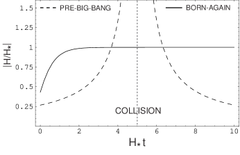
Figure 2: The evolution of the Hubble constant in the Jordan frame. The de-Sitter spacetime is an attractor of the solution. We also ploted the pre-big-bang solution in the Einstein frame.

One can also consider the cosmological evolution of the branes in the Einstein frame. Note that the two frames are indistinguishable at present if our universe is on the positive tension brane after collision. In the Einstein frame, the brane universe is contracting before the collision and one encounters a singularity at the collision point. This resembles the pre-big-bang scenario. Thus our scenario may be regarded as a non-singular realization of the pre-big-bang scenario in the braneworld context.

7.1 Gravitational waves

Now, we shall discuss the observational consequences of the scenario. The universe rapidly converges to the de-Sitter regime in the Jordan frame. As the metric couples with the radion, the non-trivial evolution of the radion field affects the tensor perturbations. This possibility descriminates our model from the usual inflationary scenario. Let us consider the tensor perturbations in the Einstein frame:

$$ds^{2}=\alpha^{2}(\tau)\left[-d\tau^{2}+(\delta_{ij}+h_{ij})dx^{i}dx^{j}\right]$$ (51)

where $\alpha$ is the scale factor and $h_{ij}$ satisfy the transverse-traceless conditions, $h_{ij}^{,j}=h^{i}_{i}=0$. As for the gravitational tensor perturbations, we have

$$h_{k}^{\prime\prime}+2{\cal H}h_{k}^{\prime}+k^{2}h_{k}=0\ ,$$ (52)

where $h_{k}$ is the amplitude of $h_{ij}$ and ${\cal H}=\alpha^{\prime}/\alpha$. Since ${\cal H}\sim(2\tau)^{-1}$ near the collision point, $h_{k}$ has the spectral index $n=4$ for the gravitational waves (with the spectral index defined by $P_{h}(k)\propto k^{n-4}$ as in the case of scalar curvature perturbation; for the tensor perturbation, the conventional definition is $n_{T}=n-1$). Provided that inflation ends right after collision, this gives a sufficiently blue spectrum that can amplify the density parameter $\Omega_{g}$ by several order of magnitudes or more on small scales as compared to conventional inflation models. Thus, there arises a possibility that it may be detected by a space laser interferometer for low frequency gravitational waves such as LISA.

7.2 Inflaton perturbation

On the other hand, the inflaton does not couple directly with the radion field. Hence, the inflaton fluctuations are expected to give adiabatic fluctuations with a flat spectrum. To calculate the inflaton perturbation rigorously, one needs to introduce an inflaton field explicitly and consider a system of equations fully coupled with the radion and the metric perturbation. According to the estimation of the effect of the metric perturbation induced by radion fluctuations on the inflaton perturbation, the inflaton fluctuations are not much affected by the radion fluctuations [7]. Thus, the inflaton fluctuations will have a standard scale-invariant spectrum.

8 Conclusion

The general formalism for studying an inflationary scenario in the two-brane system is presented. The gradient expansion method played a central role. In particular, the second order action for the cosmological perturbations has been derived. This result should be useful when we discuss the quantization of the cosmological fluctuations. As an application, we have proposed a born-again braneworld scenario. As our braneworld is inflating and the inflaton has essentially no coupling with the radion field, the adiabatic density perturbation with a flat spectrum is naturally realized. While, as the collision of branes mimics the pre-big-bang scenario [2], the primordial background gravitational waves with a very blue spectrum may be produced. This brings up the possibility that we may be able to see the collision epoch by a future gravitational wave detector such as LISA.

References

• [1] L. Randall and R. Sundrum, Phys. Rev. Lett.  83, 3370 (1999) [arXiv:hep-ph/9905221].
• [2] M. Gasperini and G. Veneziano, Astropart. Phys.  1, 317 (1993) [arXiv:hep-th/9211021].
• [3] R. Maartens, D. Wands, B. A. Bassett and I. Heard, Phys. Rev. D 62, 041301 (2000) [arXiv:hep-ph/9912464].
• [4] S. Kobayashi, K. Koyama and J. Soda, Phys. Lett. B 501, 157 (2001) [arXiv:hep-th/0009160]; Y. Himemoto and M. Sasaki, Phys. Rev. D 63, 044015 (2001) [arXiv:gr-qc/0010035].
• [5] S. Kanno and J. Soda, Phys. Rev. D 66, 043526 (2002) [arXiv:hep-th/0205188]; S. Kanno and J. Soda, Phys. Rev. D 66, 083506 (2002) [arXiv:hep-th/0207029]; S. Kanno and J. Soda, Gen. Rel. Grav.  36, 689 (2004) [arXiv:hep-th/0303203]; S. Kanno and J. Soda, Phys. Lett. B 588, 203 (2004) [arXiv:hep-th/0312106].
• [6] S. Kanno and J. Soda, Astrophys. Space Sci.  283, 481 (2003) [arXiv:gr-qc/0209087]; J. Soda and S. Kanno, Astrophys. Space Sci.  283, 639 (2003) [arXiv:gr-qc/0209086]; T. Wiseman, Class. Quant. Grav.  19, 3083 (2002) [arXiv:hep-th/0201127]; T. Shiromizu and K. Koyama, Phys. Rev. D 67, 084022 (2003) [arXiv:hep-th/0210066].
• [7] S. Kanno, M. Sasaki and J. Soda, Prog. Theor. Phys.  109, 357 (2003) [arXiv:hep-th/0210250].