Full causal bulk viscous LRS Bianchi I with time varying constants

Abstract

In this paper we study the evolution of a LRS Bianchi I Universe, filled with a bulk viscous cosmological fluid in the presence of time varying constants “but” taking into account the effects of a c-variable into the curvature tensor. We find that the only physical models are those which “constants” $G$ and $c$ are growing functions on time $t$, while the cosmological constant $\Lambda$ is a negative decreasing function. In such solutions the energy density obeys the ultrastiff matter equation of state i.e. $\omega=1$.

I Introduction

In a recent paper (Tony1 )we have studied the behaviour of the constants $G,c$ and $\Lambda$ within the framework of a flat FRW cosmological model where we consider the effects of a c-variable into the curvature tensor. The study was restricted to the perfect fluid case. In such paper we arrived to the conclusion that we have only two physical solutions and furthermore both solutions follow a power-law time dependence of the physical quantities on the cosmological time while in the previous works, where we have not taken into account the effects of a c-variable into the curvature tensor, we were capable of obtaining more solutions. We would like to emphasize that in such study we obtained as integration condition that both “constants”, in spite of considering that they vary, verify the relationship $G/c^{2}=const.$ for all equation of state. Nevertheless we have not been able to find any physical restriction in the parameters to determine if the “constants” are growing or decreasing functions on time $t,$ since both cases are permissible. We would like to point out this fact, since “traditionally” until now all the solutions obtained for both “constants” (when they vary simultaneously) are decreasing on time $t.$ In such works it was not considered the possible effects of a c-variable into the curvature tensor in such a way that the traditional FRW equations remain unalterable.

In the present paper we try to generalize the study begun in (Tony1 ) considering a cosmological model with symmetries LRS Bianchi I with variable constants and which momentum-energy tensor is modeled by a bulk viscous fluid (full causal theory) in such a way and expecting that the thermodynamics help us to restrict the parameters to find physical solutions. Furthermore bulk viscosity is expected to play an important role in the early evolution of the Universe, when also the dynamics of the “constants” $G,c$ and $\Lambda$ could be different. We shall consider the possible effects of a c-variable into the curvature tensor in such a way that we shall outlined a new field equations and we shall study the Krestchmann invariants as well as the expansion and the shear. Once the field equations have been outlined we will need to make simplifying hypotheses in order to try to obtain a complete solution to the field equations.

Under the assumed hypotheses we will study three different models finding that the physically reasonable models (decreasing temperature, increasing entropy, negative viscous pressure etc…) are those with $G$ and $c$ as growing function on time $t$ and in particular such models have an equation of the state $\omega=1$ that is to say, ultrastiff matter, and the viscous parameter is $\gamma=1/2$, the usual one. In such solutions the cosmological “constant” is a negative decreasing function. The models which have decreasing functions $G$ and $c$ result without any physical sense i.e. positive viscous pressure, decreasing entropy etc…. We end the paper summarizing all these results.

II The model and the hypotheses

A locally rotationally symmetric (LRS) Bianchi I (Ha ; Prad ) spacetime with metric

$$ds^{2}=-c^{2}(t)dt^{2}+X^{2}(t)dx^{2}+Y^{2}(t)\left(dy^{2}+dz^{2}\right),$$ (1)

filled with a bulk viscous cosmological fluid with the following energy-momentum tensor Ma95 ; Ma96 :

$$T_{i}^{k}=\left(\rho+p+\Pi\right)u_{i}u^{k}-\left(p+\Pi\right)\delta_{i}^{k},$$ (2)

where $\rho$ is the energy density, $p$ the thermodynamic pressure, $\Pi$ is the bulk viscous pressure and $u_{i}$ is the four velocity satisfying the condition $u_{i}u^{i}=-1$. The number $4-$flux and the entropy $4-$flux take the form:

$$N^{i} =nu^{i},$$ (3)

$$S^{i} =sN^{i}-\left(\frac{\tau\Pi^{2}}{2\xi T}\right)u^{i},$$ (4)

where $n$ is the number density, $s$ the specific entropy, $T\geq 0$ the temperature, $\xi$ the bulk viscosity coefficient and $\tau\geq 0$ the relaxation coefficient for transient bulk viscous effect (i.e. the relaxation time).

The fundamental thermodynamic tensors (2-4) are subject to the dynamical laws of energy-momentum conservation, number conservation and the Gibb’s equation:

$$T_{i;k}^{k} =0,$$ (5)

$$N_{\text{ };i}^{i} =0,$$ (6)

$$Tds =d\left(\frac{\rho}{n}\right)+pd\left(\frac{1}{n}\right).$$ (7)

The equations (2-4) and (5-7) imply:

$$TS_{;i}^{i}=-\Pi\left(3H+\frac{\dot{\tau}}{\xi}\dot{\Pi}+\frac{1}{2}T\Pi\left(\frac{\tau}{\xi T}u^{i}\right)_{;i}\right),$$ (8)

(where $3H=u_{;i}^{i})$ by equations (5-7) and (8), the simplest way (linear in $\Pi)$ to satisfy the $H$-theorem (i.e. for the entropy production to be non-negative, $S_{;i}^{i}=\frac{\Pi^{2}}{\xi T}\geq 0$ $)$ leads to the causal evolution equation for bulk viscosity given by Ma95

$$\tau\dot{\Pi}+\Pi=-3\xi H-\frac{\epsilon}{2}\tau\Pi\left(3H+\frac{\dot{\tau}}{\tau}-\frac{\dot{\xi}}{\xi}-\frac{\dot{T}}{T}\right),$$ (9)

In eq.(9), $\epsilon=0$ gives  the truncated theory (the truncated theory implies a drastic condition on the temperature), while $\epsilon=1$ gives the full theory. The non-causal theory has $\tau=0$.

The growth of the total commoving entropy $\Sigma=snV$ over a proper time interval $\left(t_{0},t\right)$ is given by Ma95 :

$$\Sigma(t)-\Sigma\left(t_{0}\right)=-\frac{3}{k_{B}}\int_{t_{0}}^{t}\frac{\Pi HV}{T}dt,$$ (10)

where $k_{B}$ is the Boltzmann’s constant, and $V=\left(XY^{2}\right)$ is the proper volume.

The Einstein gravitational field equations with variable $G$, $c$ and $\Lambda$ are:

$$R_{ik}-\frac{1}{2}g_{ik}R=\frac{8\pi G(t)}{c^{4}\left(t\right)}T_{ik}+\Lambda(t)g_{ik}.$$ (11)

Applying the covariance divergence to the second member of equation (11) we get:

$$div\left(\frac{G}{c^{4}}T_{i}^{j}+\delta_{i}^{j}\Lambda\right)=0,$$ (12)

$$T_{i;j}^{j}=\left(\frac{4c_{,j}}{c}-\frac{G_{,j}}{G}\right)T_{i}^{j}-\frac{c^{4}\delta_{i}^{j}\Lambda_{,j}}{8\pi G},$$ (13)

that simplifies to:

$$\dot{\rho}+3\left(\rho+p\right)H+3H\Pi=-\frac{\overset{\cdot}{\Lambda}c^{4}}{8\pi G}-\rho\frac{\dot{G}}{G}-4\rho\frac{\dot{c}}{c},$$ (14)

Therefore, our model (with LRS BI symmetries) is described by the following equations:

$$2\frac{\dot{X}}{X}\frac{\dot{Y}}{Y}+\frac{\dot{Y}^{2}}{Y^{2}} =\frac{8\pi G}{c^{2}}\rho+\Lambda c^{2},$$ (15)

$$2\frac{\ddot{Y}}{Y}+\frac{\dot{Y}^{2}}{Y^{2}}-2\frac{\dot{Y}}{Y}\frac{\dot{c}}{c} =-\frac{8\pi G}{c^{2}}\left(p+\Pi\right)+\Lambda c^{2},$$ (16)

$$\frac{\ddot{Y}}{Y}+\frac{\dot{X}}{X}\frac{\dot{Y}}{Y}+\frac{\ddot{X}}{X}-\left(\frac{\dot{X}}{X}+\frac{\dot{Y}}{Y}\right)\frac{\dot{c}}{c} =-\frac{8\pi G}{c^{2}}\left(p+\Pi\right)+\Lambda c^{2},$$ (17)

$$\dot{\rho}+\left(\rho+p+\Pi\right)\left(\frac{\dot{X}}{X}+2\frac{\dot{Y}}{Y}\right) =-\frac{\dot{\Lambda}c^{4}}{8\pi G}-\rho\frac{\dot{G}}{G}+4\rho\frac{\dot{c}}{c},$$ (18)

$$\tau\dot{\Pi}+\Pi+\xi\left(\frac{\dot{X}}{X}+2\frac{\dot{Y}}{Y}\right) =-\frac{\epsilon}{2}\tau\Pi\left(\left(\frac{\dot{X}}{X}+2\frac{\dot{Y}}{Y}\right)+\frac{\dot{\tau}}{\tau}-\frac{\dot{\xi}}{\xi}-\frac{\dot{T}}{T}\right).$$ (19)

In order to close the system of equations (15-19) we have to give the equation of state for $p$ and specify $T$, $\xi$ and $\tau$. As usual, we assume the following phenomenological (ad hoc) laws Ma95 :

$$p =\omega\rho,$$ (20)

$$\xi =k_{\gamma}\rho^{\gamma},$$ (21)

$$T =D_{\delta}\rho^{\delta},$$ (22)

$$\tau =\xi\rho^{-1}=k_{\gamma}\rho^{\gamma-1},$$ (23)

where $0\leq\omega\leq 1$, and $k_{\gamma}\geq 0$, $D_{\delta}\geq 0$ are dimensional constants, $\gamma\geq 0$ and $\delta\geq 0$ are numerical constants. Eqs. (20) are standard in cosmological models whereas the equation for $\tau$ is a simple procedure to ensure that the speed of viscous pulses does not exceed the speed of light. These are without sufficient thermodynamical motivation, but, in absence of better alternatives, we use these equations and expect that they will at least provide an indication of the range of possibilities. For the temperature law, we take, $T=D_{\delta}\rho^{\delta}$, which is the simplest law guaranteeing positive heat capacity.

In the context of irreversible thermodynamics $p$, $\rho$, $T$ and the particle number density $n$ are equilibrium magnitudes which are related by equations of state of the form $\rho=\rho(T,n)$ and $p=p(T,n)$. From the requirement that the entropy is a state function, we obtain the equation

$$\left(\frac{\partial\rho}{\partial n}\right)_{T}=\frac{p+\rho}{n}-\frac{T}{n}\left(\frac{\partial p}{\partial T}\right)_{n}.$$ (24)

For the equations of state (20-23) this relation imposes the constraint $\delta=\frac{\omega}{\omega+1}$ so that $0\leq\delta\leq 1/2$ for $0\leq\omega\leq 1$, a range of values which is usually considered in the physical literature .

The Israel-Stewart-Hiscock theory is derived under the assumption that the thermodynamical state of the fluid is close to equilibrium, that is, the non-equilibrium bulk viscous pressure should be small when compared to the local equilibrium pressure $\left|\Pi\right|<<p=\omega\rho$ . If this condition is violated then one is effectively assuming that the linear theory holds also in the nonlinear regime far from equilibrium. For a fluid description of the matter, this condition should be satisfied.

Therefore, with all these assumptions and taking into account the conservation principle, i.e., $div(T_{i}^{j})=0$, the resulting field equations are as follows:

$$2\frac{\dot{X}}{X}\frac{\dot{Y}}{Y}+\frac{\dot{Y}^{2}}{Y^{2}} =\frac{8\pi G}{c^{2}}\rho+\Lambda c^{2},$$ (25)

$$2\frac{\ddot{Y}}{Y}+\frac{\dot{Y}^{2}}{Y^{2}}-2\frac{\dot{Y}}{Y}\frac{\dot{c}}{c} =-\frac{8\pi G}{c^{2}}\left(p+\Pi\right)+\Lambda c^{2},$$ (26)

$$\frac{\ddot{Y}}{Y}+\frac{\dot{X}}{X}\frac{\dot{Y}}{Y}+\frac{\ddot{X}}{X}-\left(\frac{\dot{X}}{X}+\frac{\dot{Y}}{Y}\right)\frac{\dot{c}}{c} =-\frac{8\pi G}{c^{2}}\left(p+\Pi\right)+\Lambda c^{2},$$ (27)

$$\dot{\rho}+\left(\omega+1\right)\rho\left(\frac{\dot{X}}{X}+2\frac{\dot{Y}}{Y}\right) =-\left(\frac{\dot{X}}{X}+2\frac{\dot{Y}}{Y}\right)\Pi,$$ (28)

$$\frac{\dot{\Lambda}c^{4}}{8\pi G}+\rho\frac{\dot{G}}{G}-4\rho\frac{\dot{c}}{c} =0,$$ (29)

$$\dot{\Pi}+\frac{\Pi}{k_{\gamma}\rho^{\gamma-1}}+\rho\left(\frac{\dot{X}}{X}+2\frac{\dot{Y}}{Y}\right) =-\frac{1}{2}\Pi\left(\left(\frac{\dot{X}}{X}+2\frac{\dot{Y}}{Y}\right)-W\frac{\dot{\rho}}{\rho}\right),$$ (30)

where $W=\left(\frac{2\omega+1}{\omega+1}\right)$.

Since we have defined the $4-$velocity as:

$$u^{i}=\left(\frac{1}{c(t)},0,0,0\right)\text{ \ \ \ \ \ \ \ / \ \ \ \ \ \ \ }u^{i}u_{j}=-1$$ (31)

then the expansion is defined as follows

$$\theta:=u_{\,;\,i}^{i}\text{, \ \ \ \ \ \ \ \ \ }\theta=\frac{1}{c(t)}\left(\frac{\dot{X}}{X}+2\frac{\dot{Y}}{Y}\right)$$ (32)

and the shear is

$$\sigma^{2}=\frac{1}{2}\sigma_{ij}\sigma^{ij},\text{ \ \ \ \ \ \ }\sigma=\frac{\sqrt{3}}{3c(t)}\left(\frac{\dot{X}}{X}-\frac{\dot{Y}}{Y}\right)$$ (33)

Curvature is described by the tensor field $R_{jkl}^{i}.$ It is well know that if one uses the singular behaviour of the tensor components  or its derivates as a criterion for singularities, one gets into trouble since the singular behaviour of the coordinates or the tetrad basis rather than the curvature tensor. To avoid this problem, one should examine the scalars formed out of the curvature. The invariants $K_{1}$ and $K_{2}$ (the Kretschmann scalars) are very useful for the study of the singular behaviour:

$$K_{1} : =R_{ijkl}R^{ijkl}=\frac{4}{c^{4}}\left[\left(\frac{\ddot{X}}{X}\right)^{2}-2\frac{\ddot{X}}{X}^{2}\frac{\dot{c}\dot{X}}{cX}+\frac{\dot{c}^{2}\dot{X}^{2}}{c^{2}X^{2}}+2\left(\frac{\ddot{Y}}{Y}\right)^{2}-\right.$$ (35)

$$\left.-4\frac{\ddot{Y}}{Y}\frac{\dot{Y}}{Y}\frac{\dot{c}}{c}+\left(\frac{\dot{Y}\dot{c}}{Yc}\right)^{2}+2\left(\frac{\dot{X}}{X}\frac{\dot{Y}}{Y}\right)^{2}+\left(\frac{\dot{Y}}{Y}\right)^{4}\right]$$

$$K_{2} : =R_{ij}R^{ij}=\frac{2}{c^{4}}\left[\left(\frac{\ddot{X}}{X}\right)^{2}+\left(\frac{\dot{c}\dot{X}}{cX}\right)^{2}-2\frac{\ddot{X}}{X}^{2}\frac{\dot{c}\dot{X}}{cX}+3\left(\frac{\dot{X}}{X}\frac{\dot{Y}}{Y}\right)^{2}+\left(\frac{\dot{Y}}{Y}\right)^{4}+3\left(\frac{\ddot{Y}}{Y}\right)^{2}\right.$$ (39)

$$+3\left(\frac{\dot{Y}}{Y}\frac{\dot{c}}{c}\right)^{2}-6\frac{\ddot{Y}}{Y}\frac{\dot{Y}}{Y}\frac{\dot{c}}{c}+2\frac{\ddot{X}}{X}\frac{\ddot{Y}}{Y}-2\frac{\ddot{X}}{X}\frac{\dot{Y}}{Y}\frac{\dot{c}}{c}-2\frac{\ddot{Y}}{Y}\frac{\dot{c}\dot{X}}{cX}+2\frac{\dot{X}}{X}\frac{\dot{Y}}{Y}\left(\frac{\dot{c}}{c}\right)^{2}+$$

$$+2\frac{\dot{X}}{X}\frac{\dot{Y}}{Y}\frac{\ddot{X}}{X}-2\left(\frac{\dot{X}}{X}\right)^{2}\frac{\dot{Y}}{Y}\frac{\dot{c}}{c}+2\frac{\ddot{Y}}{Y}\left(\frac{\dot{Y}}{Y}\right)^{2}+2\frac{\ddot{Y}}{Y}\frac{\dot{Y}}{Y}\frac{\dot{X}}{X}-2\frac{\dot{X}}{X}\left(\frac{\dot{Y}}{Y}\right)^{2}\frac{\dot{c}}{c}-$$

$$\left.-2\left(\frac{\dot{Y}}{Y}\right)^{3}\frac{\dot{c}}{c}+2\left(\frac{\dot{Y}}{Y}\right)^{3}\frac{\dot{X}}{X}\right]$$

II.1 Simplifying hypotheses

In order to solve these equations we will need to make the following simplifying hypotheses:

1. We assume a relationship between the spatial directions

   $$X\thickapprox Y^{n}$$ (40)

   with $n\neq 1,$ and we will impose that the bulk viscous pressure follows a similar behavior as the energy density i.e.

   $$\Pi\thickapprox\rho,$$ (41)

   since $\left[\Pi\right]=\left[\rho\right].$

   The bulk viscous pressure and the energy density of the cosmological fluid are proportional to each other and hence, the general evolution of $\Pi$ is qualitatively similar to the evolution of the thermodynamic pressure $p$, both obeying a similar equation of state. In fact, by defining an effective coefficient $\omega_{eff}=\omega-\varkappa$, the equation of state of the cosmological fluid can be formally written as $p_{eff}=p+\Pi=\left(\omega_{eff}-1\right)\rho$. However, since the bulk viscous pressure of the cosmological fluid must also satisfy the evolution equation (30), the resulting time evolution depends not only on $\omega_{eff}$, but also, via the coefficients $\delta$ and $\gamma$, on the equations of state of the bulk viscosity coefficient, $\xi=\xi\left(\rho\right)$ and of the temperature, $T=T\left(\rho\right)$. Therefore, even that formally one can introduce an effective pressure (including both $p$ and $\Pi$), obeying a $\omega$-law equation of state, due to the extra-constraints imposed by the requirements of the causal bulk evolution, the general dynamics of the present model cannot be reduced to a perfect fluid model evolution.

2. As in previous works Ha ; M , but here, with the difference of considering a c-variable, we see from the equations (26) and (27) that it is obtained

   $$\frac{\ddot{Y}}{Y}+\frac{\dot{Y}^{2}}{Y^{2}}+\left(\frac{\dot{X}}{X}-\frac{\dot{Y}}{Y}\right)\frac{\dot{c}}{c}-\frac{\dot{X}}{X}\frac{\dot{Y}}{Y}-\frac{\ddot{X}}{X}=0$$ (42)

   1. then we can make the next hypothesis: we impose that (as in the above case)

      $$X\thickapprox Y^{n},$$ (43)

      therefore equation (42) yields

      $$\ddot{Y}=\left(\frac{n^{2}-1}{1-n}\right)\frac{\dot{Y}^{2}}{Y}+\dot{Y}\frac{\dot{c}}{c}$$ (44)

      obtaining a trivial solution

      $$Y=\left(C_{2}(n+2)+C_{1}(n+2)\int c(t)dt\right)^{\frac{1}{(n+2)}}$$ (45)

      then we will need to make a hypothesis about the behaviour of $c(t)$ in order to obtain a complete solution.

   2. if we make the next assumption

      $$c(t)=c_{0}Y^{n}$$ (46)

      then eq. (42) has the following solution:

      $$Y=X\left(C_{2}\left(n-2\right)\int X^{n-3}dt+C_{1}(2-n)\right)^{\frac{1}{2-n}}$$ (47)

      then we will need to make a hypothesis about the behaviour of $X(t)$ in order to obtain a complete solution.

In the subsequent sections we shall study three different models which correspond to each one of the hypotheses.

III Solutions

III.1 Model 1. Hypotheses 1.

We formalize this relationship in the following way, $\Pi=\varkappa\rho$, and under physical considerations we take $\varkappa\in\mathbb{R}^{-}$ and $\left|\varkappa\right|\ll 1$ Zi96 ; Zi04 .

In this section, we integrate the field equations with these assumptions and taking into account the conservation principle. This leads us to the following relationship, since

$$X\thickapprox Y^{n}\Longrightarrow\dot{\rho}+\left(\omega+1+\varkappa\right)\rho(n+2)\left(\frac{\dot{Y}}{Y}\right)=0.$$ (48)

This trivially lead us to the well known relationship between the energy density $\rho$ and the scale factor $Y$

$$\rho=A_{\omega}Y^{-\left(\omega+1+\varkappa\right)(n+2)}\text{ \ \ \ or \ \ \ \ \ }\rho=A_{\omega}Y^{-\alpha},$$ (49)

where $\alpha=\left(\omega+1+\varkappa\right)(n+2).$ It is observed that if $n=1$, we recover the standard FRW model.

Now, taking into account the eq. (30)  and simplifying it, we obtain,

$$\varkappa\dot{\rho}+\frac{\varkappa\rho}{k_{\gamma}\rho^{\gamma-1}}=\frac{\left(n+2\right)}{\alpha}\dot{\rho}-\frac{1}{2}\varkappa\dot{\rho}\left(-\frac{\left(n+2\right)}{\alpha}-W\right),$$ (50)

thereby obtaining $\rho=\rho(t).$ On simplifying further, we obtain,

$$\frac{\dot{\rho}}{\rho^{2-\gamma}}=\frac{K}{k_{\gamma}}\text{ \ \ \ }\Longrightarrow\text{ \ \ \ }\rho=dk_{\gamma}^{-b}t^{b},$$ (51)

where

$$\text{\ \ \ }K=\left(\frac{\varkappa}{\frac{\left(n+2\right)}{\alpha}+\frac{\left(n+2\right)\varkappa}{2\alpha}+\frac{W\varkappa}{2}-\varkappa}\right),\text{ \ }d=\left(\gamma-1\right)K^{b}\text{\ and \ \ \ \ }b=\frac{1}{\gamma-1}.$$ (52)

From equation (49) we obtain:

$$Y=\left(\frac{A_{\omega}}{d}k_{\gamma}^{b}t^{-b}\right)^{1/\alpha},\text{ \ \ i.e. \ \ }Y\propto t^{\frac{-1}{\left(\omega+1+\varkappa\right)\left(\gamma-1\right)\left(n+2\right)}}.$$ (53)

An important observational quantity is the deceleration parameter $q=\frac{d}{dt}\left(\frac{1}{H}\right)-1$, where $H=\frac{1}{3}\sum_{i}\frac{\dot{a}_{i}}{a_{i}}=\frac{1}{3}\left(\frac{\dot{X}}{X}+2\frac{\dot{Y}}{Y}\right),$ in this case $H=\frac{n+2}{3}\frac{\dot{Y}}{Y}.$ The sign of the deceleration parameter indicates whether the model inflates or not. The positive sign of $q$ corresponds to “standard” decelerating models whereas the negative sign indicates inflation. In our model, the deceleration parameter behaves as:

$$q=-1-\frac{3\alpha}{b(n+2)}.$$ (54)

Thus, for the parameters $\gamma,\omega$ and $\varkappa$, the deceleration parameter indicates an inflationary behaviour when 3$\alpha/b(n+2)>0$ and a non-inflationary behaviour for $\alpha/b(n+2)<-1$.

We proceed with the calculation of the other physical quantities as under:

$$\xi =k_{\gamma}\rho^{\gamma}\propto k_{\gamma}\left(dk_{\gamma}^{-b}t^{b}\right)^{\gamma}=d^{\gamma}k_{\gamma}^{1-b\gamma}t^{\gamma b},$$ (55)

$$T =D_{\delta}\rho^{\delta}=D_{\delta}\left(dk_{\gamma}^{-b}t^{b}\right)^{\delta}\text{ \ \ \ with \ \ }\delta=\frac{\omega}{\omega+1},$$ (56)

$$\tau =\xi\rho^{-1}=k_{\gamma}\left(dk_{\gamma}^{-b}t^{b}\right)^{\left(\gamma-1\right)},\text{ i.e. }\tau=d^{\gamma-1}t.$$ (57)

We see from $\tau=d^{\gamma-1}t$ that this result is in agreement with the theoretical result obtained in Ma95 . For viscous expansion to be non-thermalizing, we should have $\tau<t,$ or otherwise the basic interaction rate for viscous effects should be sufficiently rapid to restore the equilibrium as the fluid expands.

The comoving entropy is taking into account the relationship

$$\Sigma(t)-\Sigma\left(t_{0}\right)=\frac{\varkappa(n+2)}{d^{\frac{(n+2)b}{\alpha}+\delta-1}}\frac{A_{\omega}^{(n+2)/\alpha}}{\alpha k_{B}D_{\delta}}\frac{k_{\gamma}^{b(\delta+\frac{n+2}{\alpha}-1)}}{(1-\frac{n+2}{\alpha}-\delta)}\left[\tilde{t}^{b(1-\frac{n+2}{\alpha}-\delta)}\right]_{t_{0}}^{t},$$ (58)

$$\Sigma(t)-\Sigma\left(t_{0}\right)=\Sigma_{0}\left[\tilde{t}^{b(1-\frac{n+2}{\alpha}-\delta)}\right]_{t_{0}}^{t}$$ (59)

We notice that the parameter $\varkappa$ weakly perturbs the perfect fluid FRW Universe. When $\varkappa=0$, the comoving entropy assumes a constant value and we recover the perfect fluid case. Finally, we will use the equations

$$\left(2n+1\right)\frac{\dot{Y}^{2}}{Y^{2}} =\frac{8\pi G}{c^{2}}\rho+\Lambda c^{2},$$ (60)

$$\frac{\dot{\Lambda}c^{4}}{8\pi G\rho}+\frac{\dot{G}}{G}-4\frac{\dot{c}}{c} =0,$$ (61)

to obtain the behaviour of the “constants” $G,c$ and $\Lambda.$ From (60), we obtain $\dot{\Lambda}$ and using it in eq. (61) we obtain

$$\frac{\left(2n+1\right)\beta^{2}}{4\pi d}\frac{c^{2}t^{-2-b}}{Gk_{\gamma}^{-b}}\left[\frac{\dot{c}}{c}+\frac{1}{t}\right]+\frac{b}{t}=0,$$ (62)

where $\beta=-b/\alpha.$ This is a Bernouilli ode and its solution is:

$$c(t)^{2}=-\frac{1}{t^{2}}\frac{2bk_{\gamma}^{-b}}{\left(2n+1\right)A}\int G(t)t^{3+b}dt$$ (63)

with $A=\frac{\beta^{2}}{4\pi d}.$ We can see that the above equation verifies the relationship

$$\frac{k_{\gamma}^{b}c^{2}}{G}=gt^{b+2}\text{ \ \ \ \ \ therefore \ }G=gk_{\gamma}^{b}c^{2}t^{-b-2},$$ (64)

$g$ being a numerical constant. It is observed that if $b=-2$ i.e. $\gamma=1/2$, we obtain $G/c^{2}=B$. We use this relation in eq.(62) obtaining

$$\frac{\dot{c}}{c}=\left(-1-\frac{b}{K_{c}}\right)t^{-1},$$ (65)

where $K_{c}=\frac{\left(2n+1\right)\beta^{2}}{4\pi dg}$, and therefore,

$$c=\tilde{K}_{c}t^{\kappa},$$ (66)

where $\tilde{K}_{c}$ is an integration constant and $\kappa=\left(-1-\frac{b}{K_{c}}\right).$

Therefore the expansion and the shear yield

$$\theta:=\frac{1}{c(t)}\left(\frac{\dot{X}}{X}+2\frac{\dot{Y}}{Y}\right)=-\frac{b\left(n+2\right)}{\tilde{K}_{c}\alpha t^{\kappa+1}}$$ (67)

and

$$\sigma=\frac{\sqrt{3}}{3c(t)}\left(\frac{\dot{X}}{X}-\frac{\dot{Y}}{Y}\right)=-\frac{\sqrt{3}}{3}\frac{b\left(n-1\right)}{\tilde{K}_{c}\alpha t^{\kappa+1}}$$ (68)

while the Kretschmann scalars are:

$$K_{1}\thickapprox C_{1}t^{-4\left(\kappa+1\right)},\text{ \ \ \ \ \ \ \ \ \ }K_{2}\thickapprox C_{2}t^{-4\left(\kappa+1\right)}$$ (69)

we have omitted all the tedious calculations.

If we impose a new assumption (which is supported by observational considerations of $\Lambda$ decaying with time and assuming a small but non-zero value) as

$$\Lambda=\frac{l}{c^{2}(t)t^{2}}\text{ }\Longrightarrow\text{ \ }\dot{\Lambda}=-\frac{2l}{c^{2}t^{2}}\left(\frac{\dot{c}}{c}+\frac{1}{t}\right),$$ (70)

we can see from eq. (60) that

$$\frac{G}{c^{2}}=\left[\frac{3\beta^{2}-l}{8\pi d}\right]k_{\gamma}^{b}t^{-b-2}=Bk_{\gamma}^{b}t^{-b-2}.$$ (71)

Taking all these relations into consideration, we use in eq.(61) to obtain

$$-\frac{l}{4\pi B}\left(\frac{\dot{c}}{c}+\frac{1}{t}\right)-2\frac{\dot{c}}{c}-\frac{b+2}{t}=0,$$ (72)

whose trivial solution is

$$c=\mathfrak{K}_{c}t^{-\mu},$$ (73)

where $\mathfrak{K}_{c}$ is an integration constant and $\mu=\left(\frac{l+4\pi K(b+2)}{l+8\pi K}\right).$

III.1.1 Conclusions for this model.

We have solved this model under the assumptions: $div(T)=0,$ $\Pi=\varkappa\rho$, with $\varkappa\in\mathbb{R}^{-}$ and valid for $\forall\gamma.$ It is observed that if $\gamma=1/2$ we obtain $G/c^{2}=const.$ as obtained as integration condition in our previous paper Tony1 .

In the considered model the evolution of the Universe starts from a singular state, as the Krestchmann scalars show us, with the energy density, bulk viscosity coefficient and cosmological constant tending to infinity. At the initial moment $t=0$ the relaxation time is $\tau=0$. Generally the behavior of the gravitational constant shows a strong dependence on the coefficient $\gamma$ entering in the equation of state of the bulk viscosity coefficient. For $\gamma=1/2$, $G/c^{2}$ is a constant during the cosmological evolution. From the singular initial state the Universe starts to expand, with the scale factors $X$ and $Y$ as a $\gamma$-dependent functions. Depending on the value of the constants in the equations of state, the cosmological evolution is non-inflationary ($q>0$ for $H_{0}<-1$) or inflationary ($q<0$ for $H_{0}>1$). Due to the proportionality between bulk viscous pressure and energy density, both inflationary and non-inflationary models are thermodynamically consistent, with the ratio of $\Pi$ and $p$ also much smaller than $1$ in the inflationary era. Generally, the cosmological constant is a decreasing function of time.

We also notice that the $\varkappa-$parameter, i.e. the causal bulk viscous effect, weakly perturbs the FRW perfect fluid solution in such a way that the comoving entropy varies with $t,$ while in the perfect fluid case, i.e. $\varkappa=0$, the comoving entropy is constant. The same considerations could be taken into account for the scale factor $Y(t)=Y_{0}t^{\frac{1}{3\left(1-\gamma\right)\left(\omega+1+\varkappa\right)\left(n+2\right)}},$ which is perturbed weakly for the bulk viscous parameter as we can see in the special case of $\gamma=1/2$, and for the $n-$parameter. The solutions obtained for the scale factor, energy density, entropy, etc. are similar “but different” to those obtained for a perfect fluid model where the $\varkappa-$parameter vanishes. We would like to point out that our model is thermodynamically consistent for the usual matter equations of state and valid for all $\gamma-$parameter, i.e. $\forall\gamma\in\left(0,1\right).$ In the same way, we can see that the viscous parameter helps us to get rid of the so-called entropy problem since in this model entropy varies with $t.$

III.2 Model 2. Hypotheses 2a.

If we follow the hypothesis $2a$ then it is observed that

$$Y=\left(C_{2}(n+2)+C_{1}(n+2)\int c(t)dt\right)^{\frac{1}{(n+2)}}$$ (74)

and making

$$c(t)=c_{0}t^{a}$$ (75)

with $a\in\mathbb{R},$ therefore

$$Y=\left(C_{2}(n+2)+C_{1}\frac{(n+2)}{a+1}t^{a+1}\right)^{\frac{1}{(n+2)}},\text{ \ \ \ \ }\Longrightarrow\text{\ \ \ }X=\left(C_{2}(n+2)+C_{1}\frac{(n+2)}{a+1}t^{a+1}\right)^{\frac{n}{(n+2)}}$$ (76)

defining

$$H=\left(\frac{\dot{X}}{X}+2\frac{\dot{Y}}{Y}\right)=\frac{\left(a+1\right)C_{1}t^{a}}{\left(C_{2}\left(a+1\right)+C_{1}t^{a+1}\right)}$$ (77)

we can calculate the deceleration parameter $q$

$$q=\frac{d}{dt}\left(\frac{3}{H}\right)-1=3\left(-a\frac{C_{2}}{C_{1}}t^{-a-1}+\frac{1}{a+1}\right)-1$$ (78)

as we can see this expression only has sense if $C_{2}=0,$ therefore

$$q=\frac{2-a}{a+1}$$ (79)

Now taking into account the expression

$$\dot{\rho}+\left(\rho+p+\Pi\right)H=0,$$ (80)

we take $\Pi$ as

$$\Pi=-\alpha\rho-\frac{\dot{\rho}}{H}$$ (81)

$\alpha=\left(\omega+1\right),$ now simplify this expression into

$$\dot{\Pi}+\frac{\Pi}{k_{\gamma}\rho^{\gamma-1}}+\rho H=-\frac{1}{2}\Pi\left(H+W\frac{\dot{\rho}}{\rho}\right)$$ (82)

with $W=\left(\frac{2\omega+1}{\omega+1}\right),$ we obtain a second order ode for $\rho(t).$

$$\ddot{\rho}=\left(\frac{\dot{H}}{H}-\frac{\rho^{1-\gamma}}{k_{\gamma}}-AH\right)\dot{\rho}-BH^{2}\rho+CH\rho^{2-\gamma}+D\frac{\dot{\rho}^{2}}{\rho}$$ (83)

where $A=\left(\frac{1}{2}+\frac{\alpha W}{2}+\alpha\right),$ $B=\left(1-\frac{\alpha}{2}\right),$ $C=\left(\frac{\alpha}{k_{\gamma}}\right),$ $D=\frac{W}{2},$ simplifying it is obtained:

$$\ddot{\rho}=\left(\frac{a}{t}-\left(A+1\right)H-\frac{\rho^{s}}{k_{\gamma}}\right)\dot{\rho}-BH^{2}\rho+CH\rho^{s+1}+D\frac{\dot{\rho}^{2}}{\rho}$$ (84)

(where $s=1-\gamma)$ which is a second order differential equation with linear symmetries.

Taking into account the standard Lie procedure 59 ; 62 to obtaining the symmetries of this ode we see that (84) only admits the following symmetry

$$\xi=-st,\text{ \ \ \ \ }\eta=\rho$$ (85)

iff $C_{2}=0,$ (as we already know) obtaining in this way the following invariant solution:

$$\frac{dt}{\left(\gamma-1\right)\left(t\right)}=\frac{d\rho}{\rho}\Longrightarrow\rho=d_{0}t^{b},\text{ \ \ \ \ \ \ \ \ \ }b=\frac{1}{\gamma-1}$$ (86)

therefore

$$\Pi=-\alpha\rho-\frac{\dot{\rho}}{H}\Longrightarrow\Pi=\Pi_{0}t^{b},\text{ \ \ \ \ \ \ \ \ }\Pi_{0}=d_{0}k_{\gamma}^{-b}\left(-\alpha-\frac{b}{a+1}\right)$$ (87)

it is observed that we have obtained the same behaviour (in order of magnitude) than the energy density, showing in this way that our first hypothesis at least has mathematical meaning. We observe that this solution only has physical sense if $a>0,$ since $\Pi<0.$

The entropy is

$$\Sigma(t)-\Sigma\left(t_{0}\right)=\Sigma_{0}\left[\tilde{t}^{b(1-\delta)+(a+1)}\right]_{t_{0}}^{t}$$ (88)

if $a>0,$ then $\Sigma$ is a growing function on time $t.$ With these restriction we find that $q$ behaves as:

$$q=\frac{2-a}{a+1}<0\text{ \ \ }\Longleftrightarrow\text{\ \ \ \ }a>2,$$ (89)

finding that this universe accelerates.

Now from eq.

$$\left(2n+1\right)\frac{\dot{Y}^{2}}{Y^{2}}=\frac{8\pi G}{c^{2}}\rho+\Lambda c^{2},$$ (90)

and defining

$$\left(2n+1\right)\frac{\dot{Y}^{2}}{Y^{2}}=f(t)$$ (91)

we obtain $\Lambda$

$$\left(f(t)-\frac{8\pi G}{c^{2}}\rho(t)\right)\frac{1}{c^{2}(t)}=\Lambda$$ (92)

and substituting this expression into

$$\frac{\dot{\Lambda}c^{4}}{8\pi G\rho}+\frac{\dot{G}}{G}-4\frac{\dot{c}}{c}=0.$$ (93)

we end obtaining the behaviour of the “constant” $G$ as:

$$G=\frac{c^{2}f}{8\pi\dot{\rho}}\left(\frac{\dot{f}}{f}-2\frac{\dot{c}}{c}\right)$$ (94)

therefore it yields

$$G=G_{0}t^{2(a-1)-b}$$ (95)

it is observed that we have again the relationship

$$\frac{G}{c^{2}}\thickapprox t^{-2-b},\text{ \ \ \ \ \ \ \ \ }\frac{G}{c^{2}}=const.\Longleftrightarrow b=-2\Longleftrightarrow\gamma=1/2.$$ (96)

Once it has been obtained $G$ then we back to eq. (92) obtaining in this way the behaviour of $\Lambda:$

$$\Lambda=\Lambda_{0}t^{-2(a+1)}$$ (97)

The behaviour of

$$K_{1}\thickapprox t^{-4(a+1)},\text{ \ \ \ \ \ \ \ \ \ \ \ }K_{2}\thickapprox t^{-4(a+1)},$$ (98)

while the expansion and the shear behaves as:

$$\theta=\frac{a+1}{K}t^{-(a+1)},$$ (99)

$$\sigma=\frac{\sqrt{3}}{3}\frac{\left(n-1\right)}{\left(n+2\right)}\left(a+1\right)t^{-(a+1)}.$$ (100)

III.2.1 Conclusion for this model. Numerical values and graphics for the main quantities.

In the first place we begin studying the behaviour of the radius of our model. For this purpose we need to fix some numerical constants as well as consider different equations of state.

In the rest of this section we shall consider the following values for the numerical constants

$$C_{1}=1,\quad C_{2}=0,\quad c_{0}=1,\quad d_{0}=1,\quad b=-2\Longleftrightarrow\gamma=\frac{1}{2}$$

and

$$\begin{array}[]{c|c|c|c}a&n&\omega&color\\ \hline\cr\frac{1}{2}&\frac{3}{2}&1&red\\ \hline\cr\frac{1}{3}&\frac{1}{2}&\frac{1}{3}&blue\\ \hline\cr 1&\frac{1}{3}&0&magenta\\ \hline\cr\frac{-1}{2}&\frac{1}{2}&1&black\end{array}$$

we have chosen the last values (black color) as pathological.

With these numerical values we can see in fig. (1) the different behaviour of our scale factors. In all the studied cases we can see that these scale factors are growing functions on time $t$. These solutions are singular as the Krestchmann invariants show us.

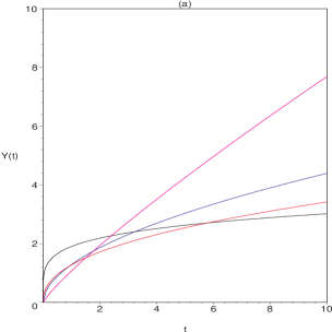
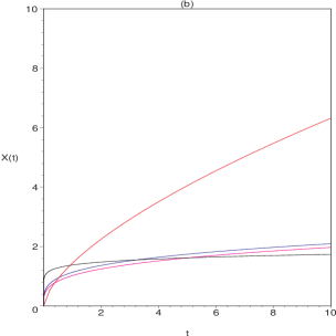
Figure 1: In the figure (a) it is plotted the radius $Y(t)$ while in figure (b) it is plotted the variation of the radius $X(t)$. Both radius have a singular start and are growing functions on time.

With regard to the energy density and the bulk viscous pressure (see fig. (2)) we can see that all the solutions have no physical meaning except the case $a=\frac{1}{2},n=\frac{3}{2}$ and $\omega=1$ (ultrastiff matter) which correspond to the red plot, since this is the only solution that verifies the condition $\Pi<0$ for all time interval and for all values of the parameters. It is observed that for $\omega=0$ (magenta line) $\Pi=0,$ i.e. $\Pi$ vanishes. Since we have only been able to obtain a particular solution (invariant solution) to the differential equation (84) for the energy density then this quantity shows the same behaviour for the chosen numerical constants.

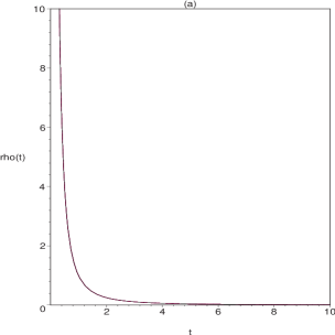
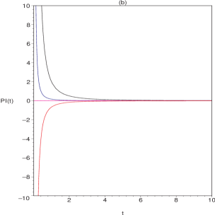
Figure 2: Figure (a) shows the variation of the energy density $\rho(t)$. Figure (b) shows the variation of the bulk viscous pressure $\Pi(t)$.

The behaviour of the thermodynamical quantities is showed in fig. (3). Even though all the studied cases show a decreasing temperature except the case $\omega=0$, magenta line, which correspond to $T(t)=const.,$ as it is expected, figure (a) shows us that only the red solution has physical sense as already we know from the last picture of the viscous pressure. This case corresponds to a growing entropy.

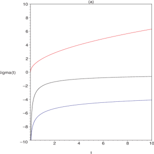
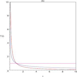
Figure 3: Figure (a) shows the variation of the entropy $\Sigma(t)$ while figure (b) shows the variation of the temperature $T(t)$.

The variation of the “constants” $G$ and $c$ as well as the relationship $G/c^{2}$ is shown in fig. (4). This figures show us that both “constants” are growing functions on time $t$ except in the case (black line) $n=-1/2$ where $G$ and $c$ are a decreasing functions on time $t$. We would like to emphasize that only for the case $\gamma=1/2$ we have that it is verified the relationship $G/c^{2}=const.$ It is a very plausible hypothesis that these effects were much stronger in the early Universe, when dissipative effects also played an important role in the dynamics of the cosmological fluid. Hence the solution obtained (red line) could give an appropriate description of the early period of our Universe.

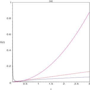
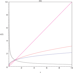
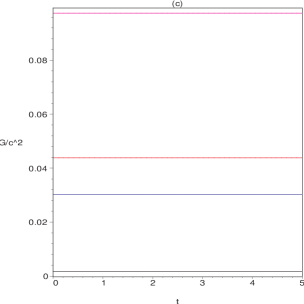
Figure 4: In the figure (a) we show the variation of “constant” $G(t)$. In the figure (b) we show the variation of the “constant” $c(t)$ and in the figure (c) it is plotted the relationship $G/c^{2}$.

With regard to the cosmological “constant”, see fig. (5), it is observed that all the solutions are decreasing but negative except for the black line ($n=-1/2).$ Maybe this fact tells us that we may consider $\Lambda(t)$ as a true ghost energy density.

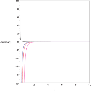
Figure 5: The variation of the cosmological “constant” $\Lambda(t)$.

The expansion and the shear behave as follows, see fig. (6). As we can see all the models studied show a decreasing expansion and the only model that has a positive shear is the plotted with the red color. The shear and expansion scalars calculated above indicate that the Universe is shearing and expanding with time. For the red color solution, the shear, which is a degree of anisotropy in the Universe, decreases monotonically with time. This indicates the fact that the initially anisotropic Universe gradually tends to an isotropic Universe at late time (present epoch) which is in agreement with the recent observations of a negligible amount of anisotropy present in the CMBR.

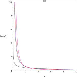
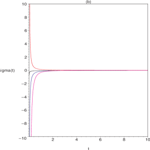
Figure 6: In figure (a) it is plotted the expansion $\theta(t)$, while in figure (b) it is plotted the shear $\sigma(t)$.

Other solutions can be studied changing the numerical values of the constants as well as taking into account different equations of state. We have found at least a physical solution (red line) which equations of state are $\omega=1$ (ultrastiff  matter) and $\gamma=1/2$ (the standard value for the viscous parameter).

III.3 Model 3. Hypotheses 2b.

If we follow the hypothesis $2b$ then it is observed that if we make the next assumption

$$c(t)=c_{0}Y^{n}$$ (101)

then eq. (42) has the following solution:

$$Y=X\left(C_{2}\left(n-2\right)\int X^{n-3}dt+C_{1}(2-n)\right)^{\frac{1}{2-n}}$$ (102)

then we will need to make a hypothesis about the behaviour of $X(t)$ in order to obtain a complete solution. Now if we assume that

$$X=Y^{m}$$ (103)

then

$$Y=\left(C_{1}\left(m-n+2\right)t+C_{2}\left(m-n+2\right)\right)^{\frac{1}{\left(m-n+2\right)}}$$ (104)

defining

$$H=\left(\frac{\dot{X}}{X}+2\frac{\dot{Y}}{Y}\right)=\frac{\left(m+2\right)C_{1}}{\left(m-n+2\right)\left(C_{1}t+C_{2}\right)}$$ (105)

we can calculate the deceleration parameter $q$

$$q=\frac{d}{dt}\left(\frac{3}{H}\right)-1=3-\frac{3n}{m+2}.$$ (106)

Now taking into account the expression

$$\dot{\rho}+\left(\rho+p+\Pi\right)H=0,$$ (107)

we take $\Pi$ as

$$\Pi=-\alpha\rho-\frac{\dot{\rho}}{H}$$ (108)

$\alpha=\left(\omega+1\right),$ now simplify this expression into

$$\dot{\Pi}+\frac{\Pi}{k_{\gamma}\rho^{\gamma-1}}+\rho H=-\frac{1}{2}\Pi\left(H+W\frac{\dot{\rho}}{\rho}\right)$$ (109)

with $W=\left(\frac{2\omega+1}{\omega+1}\right),$ we obtain a second order ode for $\rho(t).$

$$\ddot{\rho}=\left(\frac{\dot{H}}{H}-\frac{\rho^{1-\gamma}}{k_{\gamma}}-AH\right)\dot{\rho}-BH^{2}\rho+CH\rho^{2-\gamma}+D\frac{\dot{\rho}^{2}}{\rho}$$ (110)

where $A=\left(\frac{1}{2}+\frac{\alpha W}{2}+\alpha\right),$ $B=\left(1-\frac{\alpha}{2}\right),$ $C=\left(\frac{\alpha}{k_{\gamma}}\right),$ $D=\frac{W}{2},$ simplifying it is obtained:

$$\ddot{\rho}=-\left(\frac{C_{1}}{C_{1}t+C_{2}}+AH+\frac{\rho^{s}}{k_{\gamma}}\right)\dot{\rho}-BH^{2}\rho+CH\rho^{s+1}+D\frac{\dot{\rho}^{2}}{\rho}$$ (111)

(where $s=1-\gamma)$ which is a second order differential equation with linear symmetries.

Taking into account the standard Lie procedure 59 ; 62 to obtaining the symmetries of this ode we see that (111) only admits the following symmetry

$$\xi=-s\left(C_{1}t+C_{2}\right),\text{ \ \ \ \ }\eta=\rho$$ (112)

obtaining in this way the following invariant solution:

$$\frac{dt}{\left(\gamma-1\right)\left(C_{1}t+C_{2}\right)}=\frac{d\rho}{\rho}\Longrightarrow\rho=d_{0}\left(C_{1}t+C_{2}\right)^{b}$$ (113)

therefore

$$\Pi=-\alpha\rho-\frac{\dot{\rho}}{H}\Longrightarrow\Pi=\Pi_{0}\left(C_{1}t+C_{2}\right)^{b}$$ (114)

where $\Pi_{0}=-d_{0}\left(\alpha+b\left(1-\frac{n}{m+2}\right)\right).$ It is observed  the we have obtained the same behaviour (in order of magnitude) than the energy density.

The entropy is

$$\Sigma(t)-\Sigma\left(t_{0}\right)=\Sigma_{0}\left[\left(C_{1}\tilde{t}+C_{2}\right)^{b(1-\delta)+(\frac{m+2}{m-n+2})}\right]_{t_{0}}^{t}$$ (115)

Now from

$$\left(2n+1\right)\frac{\dot{Y}^{2}}{Y^{2}}=\frac{8\pi G}{c^{2}}\rho+\Lambda c^{2},$$ (116)

where

$$\left(2n+1\right)\frac{\dot{Y}^{2}}{Y^{2}}=f(t)$$ (117)

we obtain $\Lambda$

$$\left(f(t)-\frac{8\pi G}{c^{2}}\rho(t)\right)\frac{1}{c^{2}(t)}=\Lambda$$ (118)

and substituting this expression into

$$\frac{\dot{\Lambda}c^{4}}{8\pi G\rho}+\frac{\dot{G}}{G}-4\frac{\dot{c}}{c}=0.$$ (119)

we end obtaining the behaviour of the “constants”.

$$\frac{c^{2}f}{8\pi G\rho}\left(\frac{\dot{f}}{f}-2\frac{\dot{c}}{c}\right)-\frac{\dot{\rho}}{\rho}=0$$ (120)

$$G=\frac{c^{2}f}{8\pi\dot{\rho}}\left(\frac{\dot{f}}{f}-2\frac{\dot{c}}{c}\right)=G_{0}\left(C_{1}t+C_{2}\right)^{-2-b+\frac{2n}{m-n+2}}$$ (121)

with $G_{0}>0.$ It is observed that we have again the relationship

$$\frac{G}{c^{2}}\thickapprox t^{-2-b},\text{ \ \ \ \ \ \ \ \ }\frac{G}{c^{2}}=const.\Longleftrightarrow b=-2\Longleftrightarrow\gamma=1/2.$$ (122)

Once it has been obtained $G$ then we back to eq. (118) obtaining in this way the behaviour of $\Lambda:$

$$\Lambda=\Lambda_{0}\left(C_{1}t+C_{2}\right)^{\frac{-2(m+2)}{m-n+2}}$$ (123)

with $\Lambda_{0}=const.$

The behaviour of the Krestchmann scalars are:

$$K_{1}\thickapprox\left(C_{1}t+C_{2}\right)^{-\frac{4\left(n+1\right)}{m-n+2}},\text{ \ \ \ \ \ \ \ \ \ \ \ }K_{2}\thickapprox\left(C_{1}t+C_{2}\right)^{-\frac{4\left(n+1\right)}{m-n+2}},$$ (124)

while the expansion and the shear behaves as:

$$\theta=C_{1}(m+2)\left(C_{1}t+C_{2}\right)^{{}^{-\frac{m+2}{m-n+2}}},$$ (125)

$$\sigma=\frac{\sqrt{3}}{3}C_{1}\left(m-1\right)\left(C_{1}t+C_{2}\right)^{{}^{-\frac{m+2}{m-n+2}}}.$$ (126)

III.3.1 Conclusion for this model. Numerical values and graphics for the main quantities.

As in the above case we begin fixing the values of numerical constants and the equation of state. In this occasion we take for the rest of this section the following values for the numerical constants

$$C_{1}=1,\quad C_{2}=1,\quad c_{0}=1,\quad d_{0}=1,\quad b=-2\Longleftrightarrow\gamma=\frac{1}{2}$$

and

$$\begin{array}[]{c|c|c|c}n&m&\omega&color\\ \hline\cr\frac{1}{2}&\frac{3}{2}&1&red\\ \hline\cr\frac{3}{2}&\frac{1}{2}&\frac{1}{3}&blue\\ \hline\cr\frac{1}{3}&\frac{1}{3}&0&magenta\\ \hline\cr\frac{-1}{3}&\frac{1}{2}&1&black\end{array}$$

we have chosen the last values (black color) as pathological.

With these numerical values we can see in fig. (7) the different behaviour of our scale factors. In all the studied cases we can see that these scale factors are growing functions on time $t$. These solutions are non-singular as the Krestchmann invariants show us.

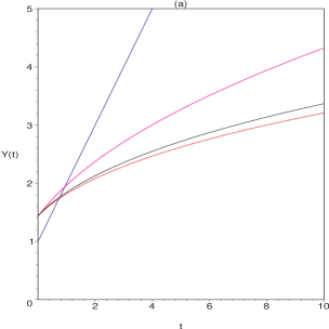
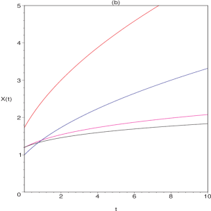
Figure 7: In the figure (a) it is plotted the radius $Y(t)$ while in figure (b) it is plotted the variation of the radius $X(t)$. Both radius have a nonsingular start and are growing functions on time.

With regard to the energy density and the viscous pressure (see fig. (8))we can see that the only solutions with physical meaning are those which have been plotted with red and blue colors i.e. with $n=\frac{1}{2},m=\frac{3}{2}$ and $\omega=1$ (ultrastiff matter) for the red color and $n=\frac{3}{2},m=\frac{1}{2}$ and $\omega=\frac{1}{3}$ for the blue line. Since we have only been able to obtain a particular solution (invariant solution) to the differential equation (111) for the energy density then this quantity shows the same behaviour for the chosen numerical constants.

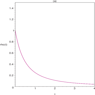
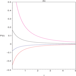
Figure 8: Figure (a) shows the variation of the energy density $\rho(t)$. Figure (b) shows the variation of the bulk viscous pressure $\Pi(t)$.

The behaviour of the thermodynamical quantities is showed in fig. (9). Even though all the studied cases shown a decreasing temperature except the case $\omega=0$, magenta line, which correspond to $T(t)=const.,$ as it is expected. Picture (a) shows us that only the red and blue solutions have physical sense as already we know from the last picture of the viscous pressure the other solutions show a decreasing entropy $\Sigma(t)$.

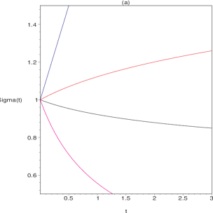
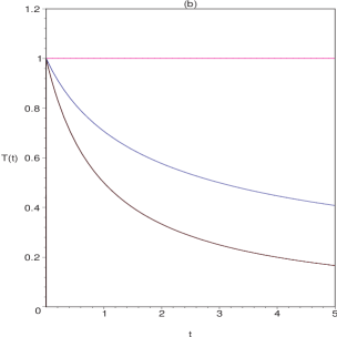
Figure 9: Figure (a) shows the variation of the entropy $\Sigma(t)$ while figure (b) shows the variation of the temperature $T(t)$.

The variation of the “constants” $G$ and $c$ as well as the relationship $G/c^{2}$ is shown in fig. (10). These pictures show us that both “constants” are growing functions on time $t$ except in the case (black line) $n=-1/2$ which correspond to a decreasing function. We would like to emphasize that only for the case $\gamma=1/2$ we have that it is verified the relationship $G/c^{2}=const.$

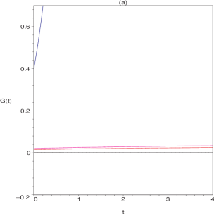
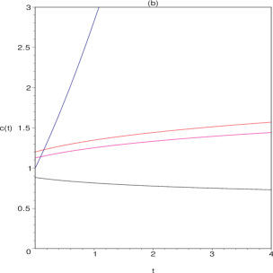
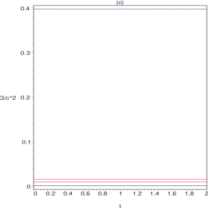
Figure 10: In the figure (a) we show the variation of “constant” $G(t)$. In the figure (b) we show the variation of the “constant” $c(t)$ and in the figure (c) it is plotted the relationship $G/c^{2}$.

With regard to the cosmological “constant”, see fig. (11), it is observed that all the solutions are decreasing but negative except for the black line ($n=-1/2).$ In these cases and because our models are non-singular $\Lambda\longrightarrow\pm const$ when $t\longrightarrow 0.$

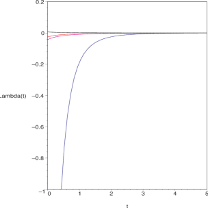
Figure 11: The variation of the cosmological “constant” $\Lambda(t)$.

The expansion and the shear behave as follows, see fig. (12). As we can see all the models studied show a decreasing expansion and only the models that have a positive shear are plotted with the red and blue colors.

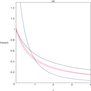
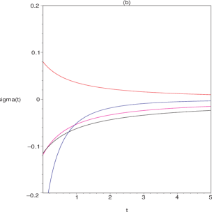
Figure 12: In figure (a) it is plotted the expansion $\theta(t)$, while in figure (b) it is plotted the shear $\sigma(t)$.

Other solutions can be studied changing the numerical values of the constants as well as taking into account different equations of state. We have found at least two non-singular physical solution (red and blue lines) which equations of state are $\omega=1$ (ultrastiff  matter) and $\omega=1/3$ with $\gamma=1/2$ (the standard value for the viscous parameter).

IV Conclusions and summary.

In this paper we have studied three different cosmological solutions for the presented model. In the first of them we have needed to make two hypotheses in order to try to obtain a complete solution of the field equations. The first assumption, $X\thickapprox Y^{n}$, is standard in this class of models while the second assumption, $\Pi\thickapprox\rho,$formalizes through the next equality, $\Pi=\varkappa\rho$, i.e. that the bulk viscous pressure has the same order of magnitude of the energy density, is more difficult of digesting. But as we have seen the other two solutions we have founded precisely this solution. We have to point out that, as we have seen, this solution is not the most general solution for the outlined differential equation. The relationship founded between the bulk viscous pressure and the energy density is the invariant solution, a particular solution. Maybe the most general solution to this ode brings us to obtain other relationship between these quantities but as it has been showed in (TonyCas ) for the classic FRW model the general solution to the outlined differential equation in the latter (see the appendix of (TonyCas )) has no physical meaning while the invariant solution (the classical solution) at least has physical sense. For all these reason together with the reasons exposed above, we believe that this hypothesis is correct.

For the first of our models we find that this is singular and thermodynamically correct since the entropy is a growing function on time $t$, if and only if $\varkappa\neq 0,$ while the temperature decreases. With regard to the behaviour of the “constants”, it is founded that the constants $G$ and $c$ for $\gamma=1/2$ must verify the relationship $G/c^{2}=const.$ in spite of the fact that both constants vary but in such a way that this quotient remains constant for all $t.$

With regard to the second of our models we can see that the red color solution which corresponds to $\omega=1$ and $\gamma=1/2$ is the only physical solution. This solution has been obtained under the assumptions that $X\thickapprox Y^{n}$ and $c\thickapprox t^{a}$, i.e. the “constant” $c(t)$, the speed of light, follows an power law dependence of time $t.$ Both hypotheses seem reasonable. The red solution is singular and both “constants” $G$ and $c$ are growing functions on time $t$ under the imposed restrictions in order to find a growing entropy $\Sigma$ and a bulk viscous pressure verifying the condition $\Pi<0.$ As we have commented above for this case it is founded that $\Pi\thickapprox\rho$, i.e. both quantities have the same order of magnitude. For the studied viscous parameter $\gamma=1/2$, and only for it, we have showed that relationship $G/c^{2}=const.$ is verified for both constants. The cosmological constant is a negative decreasing function on time $t.$

The third of our solutions is non-singular and have been obtained under the assumptions $c\thickapprox Y^{n}$ and $X\thickapprox Y^{m}.$ In this occasion we have obtained two physical solutions which correspond to the red and blue colors, with $\omega=1$ and $\omega=1/3$ respectively and in both cases the viscous parameter is $\gamma=1/2,$ the usual one. The behavior obtained for the main quantities is similar to the obtained in for the second of our models except that in this case the solutions are non-singular i.e. the constants have a growing behavior while the cosmological constant is a negative decreasing function.

Acknowledgement I wish to acknowledge to Javier Aceves his translation into English of this paper.

References

- (1) J.A. Belinchón & J.L. Caramés. “A New Formulation of a Naive Theory of Time-varying Constants.” gr-qc/0407068
- (2) J. Hajj-Botros and J. Sfeila. Inter. Jour. Theor. Phys. 26,97, (1987)
- (3) S. Ram. Inter. Jour. Theor. Phys. 28,917, (1989)
- (4) A. Mazumber. Gen. Rel. Grav. 26,307, (1994)
- (5) R.G. Vishwakarma and Abdusssatar. Phys. Rev. D 60, 063507, (1999)
- (6) I. Chakrabarty and A. Pradhan. Grav. and Cos. 7, 55, (2001).
- (7) A. Pradhan G.P. Singh and R.V. Deshpandey. “Causal Bulk Viscous LRS Bianchi I Models with Variable Gravitational and Cosmological Constants”. gr-qc/0310023
- (8) R. Maartens, Class. Quantum Grav. 12, 1455 (1995).
- (9) R. Maartens, “Causal thermodynamics in relativity”, astro-ph/9609119.
- (10) W. Israel and J.M. Stewart, Phys. Lett. A58, 213 (1976).
- (11) W. A. Hiscock and L. Lindblom, Ann. Phys. 151, 466 (1989).
- (12) W. A. Hiscock and J. Salmonson, Phys. Rev. D43, 3249 (1991)
- (13) W. Zimdahl, Phys. Rev. D53, 5483 (1996); R. Maartens and V. Mendez, Phys. Rev. D55, 1937 (1997).
- (14) R. A. Daishev and W. Zimdahl Class.Quant.Grav. 20, 5017-5024, (2003). gr-qc/0309120
- (15) N. H. Ibragimov, Elementary Lie Group Analysis and Ordinary Differential Equations (Jonh Wiley & Sons, 1999).
- (16) P. T. Olver, Applications of Lie Groups to Differential Equations (Springer-Verlang, 1993).
- (17) B. J. Cantwell, Introduction to Symmetry Analysis (Cambridge University Press, Cambridge, 2002).
- (18) G.W Bluman and S.C. Anco. “Symmetry and Integral Methods for Differential Equations”. Springer-Verlang 2002.
- (19) J.A. Belinchón. “Similarity versus Symmetries”. gr-qc/0404028.
- (20)