Vortex analogue for the equatorial geometry of the
Kerr black hole

Abstract

The spacetime geometry on the equatorial slice through a Kerr black hole is formally equivalent to the geometry felt by phonons entrained in a rotating fluid vortex. We analyse this example of “analogue gravity” in some detail: First, we find the most general acoustic geometry compatible with the fluid dynamic equations in a collapsing/expanding perfect-fluid line vortex. Second, we demonstrate that there is a suitable choice of coordinates on the equatorial slice through a Kerr black hole that puts it into this vortex form; though it is not possible to put the entire Kerr spacetime into perfect-fluid “acoustic” form. Finally, we discuss the implications of this formal equivalence; both with respect to gaining insight into the Kerr spacetime and with respect to possible vortex-inspired experiments, and indicate ways in which more general analogue spacetimes might be constructed.

1 Introduction

It is by now well-known that the propagation of sound in a moving fluid can be described in terms of an effective spacetime geometry. (See, for instance, [1, 2, 3, 4, 5, 6], and references therein).

• In the geometrical acoustics approximation, this emerges in a straightforward manner by considering the way the “sound cones” are dragged along by the fluid flow, thereby obtaining the conformal class of metrics (see, for instance, [5]):

  $$g_{\mu\nu}\propto\left[\begin{array}[]{c|c}{-\{c^{2}-h^{mn}\;v_{n}\;v_{n}}\}&-v_{j}\\ \hline\cr-v_{i}&h_{ij}\end{array}\right].$$ (1)

  Here $c$ is the velocity of sound, $v$ is the velocity of the fluid, and $h_{ij}$ is the 3-metric of the ordinary Euclidean space of Newtonian mechanics (possibly in curvilinear coordinates).

• In the physical acoustics approximation we can go somewhat further: A wave-equation for sound can be derived by linearizing and combining the Euler equation, the continuity equation, and a barotropic equation of state [1, 2, 3, 4]. For irrotational flow this process leads to the curved-space d’Alembertian equation and in particular now fixes the overall conformal factor. The resulting acoustic metric in (3+1) dimensions is (see, for instance, [4, 5]):

  $$g_{\mu\nu}=\left({\rho\over c}\right)\;\left[\begin{array}[]{c|c}{-\{c^{2}-h^{mn}\;v_{n}\;v_{n}}\}&-v_{j}\\ \hline\cr-v_{i}&h_{ij}\end{array}\right].$$ (2)

  Here $\rho$ is the density of the fluid. Sound is then described by a massless minimally coupled scalar field propagating in this acoustic geometry. In the presence of vorticity a more complicated wave equation may still be derived  [7]. For frequencies large compared to the local vorticity $\omega=||\nabla\times\vec{v}||$ that more complicated wave equation reduces to the d’Alembertian and the acoustic geometry can be identified in the usual manner. For more details see [7].

Now because the ordinary Euclidean space ($h_{ij}$) appearing in these perfect fluid acoustic geometries is Riemann flat, the 3-dimensional space (given by the constant-time slices) in any acoustic geometry is forced to be conformally flat, with 3-metric $g_{ij}=(\rho/c)\;h_{ij}$. This constraint places very strong restrictions on the class of (3+1)-dimensional geometries that can be cast into perfect fluid acoustic form. While many of the spacetime geometries of interest in general relativity can be put into this acoustic form, there are also important geometries that cannot be put into this form; at least for a literal interpretation in terms of flowing perfect fluid liquids and physical sound.

In particular, the Schwarzschild geometry can, at the level of geometrical acoustics, certainly be cast into this perfect fluid acoustic form [4]. However, at the level of physical acoustics (and working within the context of the Painléve–Gullstrand coordinates) there is a technical difficulty in that the Euler and continuity equations applied to the background fluid flow yield a nontrivial and unwanted (3+1) conformal factor $\rho/c$ [4]. This overall conformal factor is annoying, but it does not affect the sound cones, and so does not affect the “causal structure” of the resulting analogue spacetime [6]. Furthermore any overall conformal factor will not affect the surface gravity [8], so it will not directly affect the acoustic analogue of Hawking radiation [1, 4]. So for most of the interesting questions one might ask, the Schwarzschild geometry can for all practical purposes be cast into acoustic form.

Alternatively, as we shall demonstrate below, the Schwarzschild geometry can also be put into acoustic form in a different manner by using isotropic coordinates — see the appendix of this article for details. More generally, any spherically symmetric geometry (static or otherwise) can be put into acoustic form — details are again provided in the appendix. (This of course implies that the Reissner–Nordström geometry can be put into acoustic form.) In particular, the FRW cosmologies can also be put into acoustic form, both at the level of physical acoustics and at the level of geometrical acoustics. In fact there are two rather different routes for doing so: Either by causing the fluid to explode or by adjusting the speed of sound [9, 10, 11, 12, 13, 14, 15, 16].

There is however a fundamental restriction preventing the Kerr geometry [and Kerr–Newman geometry] being cast into perfect fluid acoustic form. It has recently been established [17, 18, 19] that no possible time-slicing of the full Kerr geometry can ever lead to conformally flat spatial 3-slices. Faced with this fact, we ask a more modest question: Can we at least cast a subspace of the Kerr geometry into perfect fluid acoustic form? Specifically, since we know that the effective geometry of a generalized line vortex (a “draining bathtub” geometry) contains both horizons and ergosurfaces [4, 5], one is prompted to ask: If we look at the equatorial slice of the Kerr spacetime can we at least put that into acoustic form? If so, then this opens the possibility of finding a physically reasonable analogue model based on a vortex geometry that might mimic this important aspect of the Kerr geometry. Thus we have three independent physics questions to answer:

• What is the most general perfect fluid acoustic metric that can [even in principle] be constructed for the most general [translation invariant] line vortex geometry?

• Can the equatorial slice of Kerr then be put into this form?
  (And if not, how close can one get?)

• By generalizing the analogue model to something more complicated than a perfect fluid, can we do any better?

We shall now explore these three issues in some detail.

2 Vortex flow

2.1 General framework

The background fluid flow [on which the sound waves are imposed] is governed by three key equations: The continuity equation, the Euler equation, and a barotropic equation of state:

$$\frac{\partial\rho}{\partial t}+\nabla\cdot(\rho\;\vec{v})=0.$$ (3)

$$\rho\left[\frac{\partial\vec{v}}{\partial t}+(\vec{v}\cdot\nabla)\vec{v}\right]=-\nabla p+\vec{f}.$$ (4)

$$p=p(\rho).$$ (5)

Here we have included for generality an arbitrary external force $\vec{f}$, possibly magneto-hydrodynamic in origin, that we can in principle think of imposing on the fluid flow to shape it in some desired fashion. From an engineering perspective the Euler equation is best rearranged as

$$\vec{f}=\rho\left[\frac{\partial\vec{v}}{\partial t}+(\vec{v}\cdot\nabla)\vec{v}\right]+\nabla p,$$ (6)

with the physical interpretation being that $\vec{f}$ is now telling you what external force you would need in order to set up a specified fluid flow.

2.2 Zero radial flow

Assuming now a cylindrically symmetric time-independent fluid flow without any sinks or sources we have a line vortex aligned along the $z$ axis with fluid velocity $\vec{v}$:

$$\vec{v}(r)=v_{\hat{\theta}}(r)\;\hat{\theta}.$$ (7)

The continuity equation (3) for this geometry is trivially satisfied and calculating the fluid acceleration leads to

$$\vec{a}=(\vec{v}\cdot\nabla)\vec{v}=-\frac{v_{\hat{\theta}}(r)^{2}}{r}\;\hat{r}.$$ (8)

Substituting this into the rearranged Euler equation (6) gives

$$\vec{f}=f_{\hat{r}}\;\hat{r}=\left\{-\rho(r)\;\frac{v_{\hat{\theta}}(r)^{2}}{r}+c^{2}(r)\;\partial_{r}\rho(r)\right\}\hat{r}$$ (9)

with the physical interpretation that:

• The external force $\vec{f}_{\hat{r}}$ must be chosen to precisely cancel against the combined effects of centripetal acceleration and pressure gradient. The angular-flow is not completely controlled by this external force, but is instead an independently specifiable quantity. (There is only one relationship between $f_{r}(r)$, $\rho(r)$, $c(r)$, and $v_{\theta}(r)$, which leaves three of these quantities as arbitrarily specifiable functions.)

• We are now considering the equation of state to be an output from the problem, rather than an input to the problem. If for instance $\rho(r)$ and $c^{2}(r)$ are specified then the pressure can be evaluated from

  $$p(r)=\int c^{2}(r)\;{{\mathrm{d}}\rho\over{\mathrm{d}}r}\;{\mathrm{d}}r,$$ (10)

  and then by eliminating $r$ between $p(r)$ and $\rho(r)$, the EOS $p(\rho)$ can in principle be determined.

• For zero external force (and no radial flow), which arguably is the most natural system to set up in the laboratory, we have

  $${v_{\theta}^{2}(r)\over c^{2}(r)}=r\;\partial_{r}\ln\rho(r),$$ (11)

  which still has two arbitrarily specifiable functions.

• In the geometric acoustics regime the acoustic line-element for this zero-source/ zero-sink line vortex is

  $${\mathrm{d}}s^{2} \propto -\left(c^{2}-v_{\hat{\theta}}^{2}\right){\mathrm{d}}t^{2}-2v_{\hat{\theta}}\;r\;{\mathrm{d}}\theta\;{\mathrm{d}}t+{\mathrm{d}}r^{2}+r^{2}{\mathrm{d}}\theta^{2}+{\mathrm{d}}z^{2}.$$ (12)

  In the physical acoustics regime the acoustic line-element is

  $${\mathrm{d}}s^{2}=\left(\frac{\rho}{c}\right)\Big{[}-\left(c^{2}-v_{\hat{\theta}}^{2}\right){\mathrm{d}}t^{2}-2v_{\hat{\theta}}\;r{\mathrm{d}}\theta\;{\mathrm{d}}t+{\mathrm{d}}r^{2}+r^{2}{\mathrm{d}}\theta^{2}+{\mathrm{d}}z^{2}\Big{]}.$$ (13)

  The vortex quite naturally has a ergosurface where the speed of the fluid flow equals the speed of sound in the fluid. This vortex geometry may or may not have a horizon — since $v_{\hat{r}}$ is identically zero the occurrence or otherwise of a horizon depends on whether or not the speed of sound $c(r)$ exhibits a zero. We shall later see that this class of acoustic geometries is the most natural for building analogue models of the equatorial slice of the Kerr geometry.

Figure 1: A simple non-collapsing vortex geometry: The green circles denote the streamlines of the fluid flow. The outer red circle represents the ergosurface, where the fluid velocity reaches the speed of sound. The inner red circle (which need not exist in general) represents a possible [outer] horizon where the speed of sound goes to zero.

2.3 General analysis with radial flow

For completeness we now consider the situation where the vortex contains a sink or source at the origin. (A concrete example might be the “draining bathtub” geometry where fluid is systematically extracted from a drain located at the centre.) Assuming now a cylindrically symmetric time-independent fluid flow with a line vortex aligned along the $z$ axis, the fluid velocity $\vec{v}$ is

$$\vec{v}=v_{\hat{r}}(r)\;\hat{r}+v_{\hat{\theta}}(r)\;\hat{\theta}.$$ (14)

Wherever the radial velocity $v_{\hat{r}}(r)$ is nonzero the entire vortex should be thought of as collapsing or expanding.

Figure 2: A collapsing vortex geometry (draining bathtub): The green spirals denote streamlines of the fluid flow. The outer circle represents the ergosurface while the inner circle represents the [outer] event horizon.

The continuity equation (3) for this cylindrically symmetric problem is

$$\nabla\cdot(\rho\;\vec{v})=0,$$ (15)

and the rearranged Euler equation (6) for a pressure $p$ which depends only on the radial-coordinate $r$ is

$$\vec{f}=\rho(\vec{v}\cdot\nabla)\vec{v}+c^{2}\;{\partial}_{r}\rho\;\hat{r}.$$ (16)

At this stage we note that $\rho$ is in general not an independent variable. Because equation (15) corresponds to a divergence-free field, integration over any closed circle in the two-dimensional plane yields

$$\oint\rho(r)\;\vec{v}(r)\cdot\hat{r}\;{\mathrm{d}}s=2\pi\;\rho(r)\;v_{\hat{r}}(r)\;r=2\pi\;k_{1}.$$ (17)

Then provided $v_{\hat{r}}\neq 0$,

$${\rho(r)}=\frac{k_{1}}{r\;v_{\hat{r}}(r)}.$$ (18)

Substituting into the rearranged Euler equation gives

$$\vec{f}={k_{1}\over rv_{\hat{r}}}\;(\vec{v}\cdot\nabla)\vec{v}+c^{2}\;{\partial}_{r}\left({k_{1}\over rv_{\hat{r}}}\right)\;\hat{r},$$ (19)

where $c$ is a function of $\rho$, and thus a function of $v_{\hat{r}}$. This now completely specifies the force profile in terms of the desired velocity profile, $v_{\hat{r}}$, $v_{\hat{\theta}}$, the equation of state, and a single integration constant $k_{1}$. Calculating the fluid acceleration leads to

$$(\vec{v}\cdot\nabla)\vec{v}=\left\{v_{\hat{r}}(r)\partial_{r}v_{\hat{r}}(r)-\frac{v_{\hat{\theta}}(r)^{2}}{r}\right\}\hat{r}+\left\{v_{\hat{r}}(r)\partial_{r}v_{\hat{\theta}}(r)+\frac{v_{\hat{r}}(r)\;v_{\hat{\theta}}(r)}{r}\right\}\hat{\theta},$$ (20)

which can be rearranged to yield

$$(\vec{v}\cdot\nabla)\vec{v}=\left\{{1\over 2}\partial_{r}[v_{\hat{r}}(r)^{2}]-\frac{v_{\hat{\theta}}(r)^{2}}{r}\right\}\hat{r}+\left\{{v_{\hat{r}}(r)\over r}\partial_{r}[r\;v_{\hat{\theta}}(r)]\right\}\hat{\theta}.$$ (21)

Finally, decomposing the external force into radial and tangential [torque-producing directions] we have

$$f_{\hat{r}}=\vec{f}\cdot\hat{r}=k_{1}\left\{{1\over rv_{\hat{r}}}\;\left[{1\over 2}\partial_{r}[v_{\hat{r}}(r)^{2}]-\frac{v_{\hat{\theta}}(r)^{2}}{r}\right]+c^{2}\;{\partial}_{r}\left({1\over rv_{\hat{r}}}\right)\right\},$$ (22)

and

$$f_{\hat{\theta}}=\vec{f}\cdot\hat{\theta}=k_{1}\left\{{1\over r^{2}}\partial_{r}[r\;v_{\hat{\theta}}(r)]\right\}.$$ (23)

The radial equation can undergo one further simplification to yield

$$f_{\hat{r}}=k_{1}\left\{{1\over r}\,\left[1-{c_{s}^{2}\over v_{\hat{r}}^{2}}\right]\,\partial_{r}v_{\hat{r}}-{c_{s}^{2}+v_{\hat{\theta}}^{2}\over r^{2}\;v_{\hat{r}}}\right\}.$$ (24)

Summarizing:

• In the geometric acoustics regime the acoustic line-element for the most general [time-independent cylindrically symmetric collapsing/ expanding] line vortex is

  $${\mathrm{d}}s^{2} \propto -\left(c^{2}-v_{\hat{r}}^{2}-v_{\hat{\theta}}^{2}\right){\mathrm{d}}t^{2}-2v_{\hat{r}}\;{\mathrm{d}}r\;{\mathrm{d}}t-2v_{\hat{\theta}}\;r\;{\mathrm{d}}\theta\;{\mathrm{d}}t$$ (25)

  $$\qquad+{\mathrm{d}}r^{2}+r^{2}{\mathrm{d}}\theta^{2}+{\mathrm{d}}z^{2}.$$

  We again reiterate that — given a barotropic equation of state $p(\rho)$ — once the velocity profile $v_{\hat{r}}$ and $v_{\hat{\theta}}$ is specified, then up to a single integration constant $k_{1}$, the density and speed of sound are no longer free but are fixed by the continuity equation and the equation of state respectively. Furthermore, the Euler equation then tells you exactly how much external force is required to set up the fluid flow. There are still two freely specifiable functions which we can take to be the two components of velocity.

• In the physical acoustics regime the acoustic line-element is

  $${\mathrm{d}}s^{2} = \left(\frac{\rho}{c}\right)\Big{[}-\left(c^{2}-v_{\hat{r}}^{2}-v_{\hat{\theta}}^{2}\right){\mathrm{d}}t^{2}-2v_{\hat{r}}\;{\mathrm{d}}r\;{\mathrm{d}}t-2v_{\hat{\theta}}\;r{\mathrm{d}}\theta\;{\mathrm{d}}t$$ (26)

  $$\qquad\qquad+{\mathrm{d}}r^{2}+r^{2}{\mathrm{d}}\theta^{2}+{\mathrm{d}}z^{2}\Big{]}.$$

  The major difference for physical acoustics is that for technical reasons the massless curved-space Klein–Gordon equation [d’Alembertian wave equation] can only be derived if the flow has zero vorticity. This requires $v_{\hat{\theta}}(r)=k_{2}/r$ and hence $f_{\hat{\theta}}=0$, so that the flow would be un-torqued. More precisely, the d’Alembertian wave equation is a good approximation as long as the frequency of the wave is high compared to the vorticity. However, in the presence of significant torque and vorticity, a more complicated wave equation holds [7], but that wave equation requires additional geometrical structure beyond the effective metric, and so is not suitable for developing general relativity analogue models. (Though this more complicated set of coupled PDEs is of direct physical interest in its own right.) 

There are several special cases of particular interest:

• No vorticity, $\nabla\times\vec{v}=0$;

• No angular torque, $f_{\hat{\theta}}=0$;

• No radial flow $v_{\hat{r}}=0$;

• No radial force, $f_{\hat{r}}=0$;

• No external force, $\vec{f}=0$;

which we will now explore in more detail.

Zero vorticity/ zero torque:

If we assume zero vorticity, $\nabla\times\vec{v}=0$, the above calculation simplifies considerably, since then

$$v_{\hat{\theta}}=\frac{k_{2}}{r}\;,$$ (27)

which implies $f_{\hat{\theta}}=0$. Conversely, if we assume zero torque, then (assuming $k_{1}\neq 0$) the vorticity is zero.

But note that the simple relationship zero torque $\iff$ zero vorticity requires the assumption of nonzero radial flow. With zero radial flow the torque is always zero for a time independent flow, regardless of whether or not the flow is vorticity free.

Zero radial force:

Assuming zero radial force, $f_{\hat{r}}=0$, and assuming $k_{1}\neq 0$, one finds

$${1\over rv_{\hat{r}}}\;\left[{1\over 2}\partial_{r}[v_{\hat{r}}(r)^{2}]-\frac{v_{\hat{\theta}}(r)^{2}}{r}\right]+c^{2}(r)\;{\partial}_{r}\left({1\over rv_{\hat{r}}}\right)=0.$$ (28)

Thus the radial and angular parts of the background velocity are now dependent on each other. Once you have chosen, e.g., $v_{\hat{\theta}}(r)$ and $c(r)$, a differential equation constrains $v_{\hat{r}}$:

$$v_{\hat{r}}\;\partial_{r}v_{\hat{r}}\left[1-\frac{c^{2}}{v_{r}^{2}}\right]=\frac{c^{2}+v_{\hat{\theta}}^{2}}{r}\;.$$ (29)

Zero external force:

If we assume zero external force, $\vec{f}=0$, both the radial and angular external forces are zero. Then assuming $k_{1}\neq 0$

$$v_{\hat{r}}\;\partial_{r}v_{\hat{r}}\left[1-\frac{c^{2}}{v_{r}^{2}}\right]=\frac{c^{2}}{r}+\frac{k_{2}^{2}}{r^{3}}\;.$$ (30)

Since $c$ depends on $\rho$ via the barotropic equation, and $\rho$ depends on $v_{r}$ via the continuity equation, this is actually a rather complicated nonlinear ODE for $v_{r}(r)$. (For zero radial flow this reduces to the tautology $0=0$ and we must adopt the analysis of the previous subsection.)

In general the ergosurface is defined by the location where the flow goes supersonic

$$v_{\hat{r}}^{2}+v_{\hat{\theta}}^{2}=c^{2}$$ (31)

while the horizon is defined by the location where

$$v_{\hat{r}}^{2}=c^{2}$$ (32)

Note that horizons can form in three rather different ways:

• $v_{\hat{r}}=-c\neq 0$ — a black hole horizon.

• $v_{\hat{r}}=+c\neq 0$ — a white hole horizon.

• $v_{\hat{r}}=\pm c=0$ — a bifurcate horizon.

In analogue models it is most usual to keep $c\neq 0$ and use fluid flow to generate the horizon, this is the case for instance in the Painléve–Gullstrand version of the Schwarzschild geometry [4, 5]. The alternate possibility of letting both $v_{\hat{r}}\to 0$ and $c\to 0$ to obtain a horizon is not the most obvious construction from the point of view of acoustic geometries, but cannot a priori be excluded on either mathematical or physical grounds. Indeed, it is this less obvious manner of implementing the acoustic geometry that most closely parallels the analysis of Schwarzschild black holes in curvature coordinates or isotropic coordinates, and we shall soon see that this route is preferred when investigating the Kerr spacetime.

3 The role of dimension

The role of spacetime dimension in these acoustic geometries is sometimes a bit surprising and potentially confusing. This is important because there is a real physical distinction between truly two-dimensional systems and effectively two-dimensional systems in the form of three-dimensional systems with cylindrical symmetry. We emphasise that in cartesian coordinates the wave equation

$$\frac{\partial}{\partial{x^{\mu}}}\left(f^{\mu\nu}\frac{\partial}{\partial{x^{\nu}}}\;\psi\right)=0,$$ (33)

where

$$f^{\mu\nu}=\left[\begin{array}[]{ccc}-{\rho}/{c^{2}}&|&-{\rho}\;{v^{j}}/{c^{2}}\\ \hline\cr-{\rho}\;{v^{i}}/{c^{2}}&|&\rho\;\{\delta^{ij}-v^{i}v^{j}/{c^{2}}\}\end{array}\right],$$ (34)

holds independent of the dimensionality of spacetime. It depends only on the Euler equation, the continuity equation, a barotropic equation of state, and the assumption of irrotational flow [3].

Introducing the acoustic metric $g^{\mu\nu}$, defined by

$$f^{\mu\nu}=\sqrt{-g}\,g^{\mu\nu};\qquad g=\frac{1}{\det(g^{\mu\nu})}$$ (35)

the wave equation (33) corresponds to the massless Klein–Gordon equation [d’Alembertian wave equation] in a curved space-time with contravariant metric tensor:

$$g^{\mu\nu}=\left({\rho\over c}\right)^{-2/(d-1)}\left[\begin{array}[]{c|c}-1/c^{2}&-\vec{v}^{\,T}/c^{2}\\ \hline\cr\vphantom{\Big{|}}-\vec{v}/c^{2}&\mathbf{I}_{d\times d}-\vec{v}\otimes\vec{v}^{\,T}/c^{2}\end{array}\right],$$ (36)

where $d$ is the dimension of space (not spacetime).

The covariant acoustic metric is

$$g_{\mu\nu}=\left(\frac{\rho}{c}\right)^{2/(d-1)}\left[\begin{array}[]{ccc}-\left(c^{2}-v^{2}\right)&|&-\vec{v}^{\,T}\\ \hline\cr-\vec{v}&|&\mathbf{I}_{d\times d}\end{array}\right].$$ (37)

3.1 $d=3$

The acoustic line-element for three space and one time dimension reads

$$g_{\mu\nu}=\left(\frac{\rho}{c}\right)\left[\begin{array}[]{ccc}-\left(c^{2}-v^{2}\right)&|&-\vec{v}^{\,T}\\ \hline\cr-\vec{v}&|&\mathbf{I}_{3\times 3}\end{array}\right].$$ (38)

This is the primary case of interest in this article.

3.2 $d=2$

The acoustic line-element for two space and one time dimension reads

$$g_{\mu\nu}=\left(\frac{\rho}{c}\right)^{2}\left[\begin{array}[]{ccc}-\left(c^{2}-v^{2}\right)&|&-\vec{v}^{\,T}\\ \hline\cr-\vec{v}&|&\mathbf{I}_{2\times 2}\end{array}\right].$$ (39)

This situation would be appropriate when dealing with surface waves or excitations confined to a particular substrate, for example at the surface between two superfluids. An important physical point is that, due to the fact that one can always find a conformal transformation to make the two-dimensional spatial slice flat [20], essentially all possible 2+1 metrics can in principle be reproduced by acoustic metrics [21]. (The only real restriction is the quite physical constraint that there be no closed timelike curves in the spacetime.)

3.3 $d=1$

The naive form of the acoustic metric in (1+1) dimensions is ill-defined, because the conformal factor is raised to a formally infinite power — this is a side effect of the well-known conformal invariance of the Laplacian in 2 dimensions. The wave equation in terms of $f^{\mu\nu}$ continues to make good sense — it is only the step from $f^{\mu\nu}$ to the effective metric that breaks down.

Note that this issue only presents a difficulty for physical systems that are intrinsically one-dimensional. A three-dimensional system with plane symmetry, or a two-dimensional system with line symmetry, provides a perfectly well behaved model for (1+1) dimensions, as in the cases $d=3$ and $d=2$ above.

4 The Kerr equator

To compare the vortex acoustic geometry to the physical Kerr geometry of a rotating black hole [22], consider the equatorial slice $\theta=\pi/2$ in Boyer–Lindquist coordinates [23]:

$$({\mathrm{d}}s^{2})_{(2+1)}=-{\mathrm{d}}t^{2}+{2m\over r}({\mathrm{d}}t-a\;{\mathrm{d}}\phi)^{2}+{{\mathrm{d}}r^{2}\over 1-2m/r+a^{2}/r^{2}}+(r^{2}+a^{2})\;{\mathrm{d}}\phi^{2}.$$ (40)

We would like to put this into the form of an “acoustic metric”

$$g_{\mu\nu}=\left({\rho\over c}\right)\;\left[\begin{array}[]{c|c}{-\{c^{2}-h^{mn}\;v_{n}\;v_{n}}\}&-v_{j}\\ \hline\cr-v_{i}&h_{ij}\end{array}\right].$$ (41)

If we look at the 2-d $r$-$\phi$ plane, the metric is

$$({\mathrm{d}}s^{2})_{(2)}={{\mathrm{d}}r^{2}\over 1-2m/r+a^{2}/r^{2}}+\left(r^{2}+a^{2}+{2ma^{2}\over r}\right){\mathrm{d}}\phi^{2}.$$ (42)

Now it is well-known that any 2-d geometry is locally conformally flat [20], though this fact is certainly not manifest in these particular coordinates. Introduce a new radial coordinate $\tilde{r}$ such that:

$${{\mathrm{d}}r^{2}\over 1-2m/r+a^{2}/r^{2}}+\left(r^{2}+a^{2}+{2ma^{2}\over r}\right){\mathrm{d}}\phi^{2}=\Omega(\tilde{r})^{2}\;[{\mathrm{d}}\tilde{r}^{2}+\tilde{r}^{2}\;{\mathrm{d}}\phi^{2}].$$ (43)

This implies

$$\left(r^{2}+a^{2}+{2ma^{2}\over r}\right)=\Omega(\tilde{r})^{2}\;\tilde{r}^{2},$$ (44)

and

$${{\mathrm{d}}r^{2}\over 1-2m/r+a^{2}/r^{2}}=\Omega(\tilde{r})^{2}\;{\mathrm{d}}\tilde{r}^{2},$$ (45)

leading to the differential equation

$${1\over\tilde{r}(r)}\;{{\mathrm{d}}\tilde{r}(r)\over{\mathrm{d}}r}={1\over\sqrt{1-2m/r+a^{2}/r^{2}}\sqrt{r^{2}+a^{2}+{2ma^{2}/r}}},$$ (46)

which is formally solvable as

$$\tilde{r}(r)=\exp\left\{\hbox{\Large$\displaystyle\int$}{{\mathrm{d}}r\over\sqrt{1-2m/r+a^{2}/r^{2}}\sqrt{r^{2}+a^{2}+{2ma^{2}/r}}}\right\}.$$ (47)

The normalization is most easily fixed by considering the $m=0=a$ case, in which case $\tilde{r}=r$, and then using this to write the general case as

$$\tilde{r}(r)=r\exp\left[-\int_{r}^{\infty}\left\{{1\over\sqrt{1-2m/\bar{r}+a^{2}/\bar{r}^{2}}\sqrt{\bar{r}^{2}+a^{2}+{2ma^{2}/\bar{r}}}}-{1\over\bar{r}}\right\}{\mathrm{d}}\bar{r}\right],$$ (48)

where $\bar{r}$ is simply a dummy variable of integration. If $a=0$ this integral can be performed in terms of elementary functions

$$\int{{\mathrm{d}}r\over r\sqrt{1-2m/r}}=\ln\left(\sqrt{r^{2}-2mr}+r-m\right)\qquad\qquad[r>2m],$$ (49)

so that

$$\tilde{r}(r)={{1\over 2}}\left(\sqrt{r^{2}-2mr}+r-m\right),$$ (50)

though for $m\neq 0$ and general $a$ no simple analytic form holds. Similarly, for $m=0$ and $a\neq 0$ it is easy to show that

$$\tilde{r}(r)=\sqrt{r^{2}+a^{2}},$$ (51)

though for $a\neq 0$ and general $m$ no simple analytic form holds.

Nevertheless, since we have an exact [if formal] expression for $\tilde{r}(r)$ we can formally invert it to assert the existence of a function $r(\tilde{r})$. It is most useful to write $\tilde{r}=r\;F(r)$, with $\lim_{r\to\infty}F(r)=1$, and to write the inverse function as $r=\tilde{r}\;H(\tilde{r})$ with the corresponding limit $\lim_{\tilde{r}\to\infty}H(\tilde{r})=1$. Even if we cannot write explicit closed form expressions for $F(r)$ and $H(\tilde{r})$ there is no difficulty in calculating them numerically, or in developing series expansions for these quantities, or even in developing graphical representations.

We now evaluate the conformal factor as

$$\Omega(\tilde{r})^{2}={r^{2}+a^{2}+{2ma^{2}/r}\over\tilde{r}^{2}}=H(\tilde{r})^{2}\;\left(1+{a^{2}\over r^{2}}+{2ma^{2}\over r^{3}}\right),$$ (52)

with $r$ considered as a function of $\tilde{r}$, which now yields

$$({\mathrm{d}}s^{2})_{(2+1)}=-{\mathrm{d}}t^{2}+{2m\over r}({\mathrm{d}}t^{2}-2a\;{\mathrm{d}}\phi\;{\mathrm{d}}t)+\Omega(\tilde{r})^{2}\;[{\mathrm{d}}\tilde{r}^{2}+\tilde{r}^{2}\;{\mathrm{d}}\phi^{2}].$$ (53)

Equivalently

$$({\mathrm{d}}s^{2})_{(2+1)} = \Omega(\tilde{r})^{2}\Bigg{\{}-\Omega(\tilde{r})^{-2}\left[1-{2m\over r}\right]{\mathrm{d}}t^{2}-\Omega(\tilde{r})^{-2}{4am\over r}\;{\mathrm{d}}\phi\;{\mathrm{d}}t$$ (54)

$$\qquad\qquad+[{\mathrm{d}}\tilde{r}^{2}+\tilde{r}^{2}\;{\mathrm{d}}\phi^{2}]\Bigg{\}}.$$

This now lets us pick off the coefficients of the equivalent acoustic metric. For the overall conformal factor

$${\rho\over c}=\Omega(\tilde{r})^{2}=H^{2}(\tilde{r})\;\left(1+{a^{2}\over r^{2}}+{2ma^{2}\over r^{3}}\right).$$ (55)

For the azimuthal “flow”

$$v_{\phi}=\Omega(\tilde{r})^{-2}\;{2am\over r}={2am\over r}\;H^{-2}(\tilde{r})\;\left(1+{a^{2}\over r^{2}}+{2ma^{2}\over r^{3}}\right)^{-1}.$$ (56)

In terms of orthonormal components

$$v_{\hat{\phi}}={v_{\phi}\over\tilde{r}}={2am\over r^{2}}\;H^{-1}(\tilde{r})\;\left(1+{a^{2}\over r^{2}}+{2ma^{2}\over r^{3}}\right)^{-1}.$$ (57)

This is, as expected, a vortex geometry. Finally for the “coordinate speed of light”, corresponding to the speed of sound in the analogue geometry

$$c^{2} = \Omega(\tilde{r})^{-2}\;\left[1-{2m\over r}\right]+\Omega(\tilde{r})^{-4}\;{4a^{2}m^{2}\over\tilde{r}^{2}\;r^{2}},$$ (58)

$$= \Omega(\tilde{r})^{-4}\left\{\Omega(\tilde{r})^{2}\;\left[1-{2m\over r}\right]+\;{4a^{2}m^{2}\over\tilde{r}^{2}\;r^{2}}\right\}.$$ (59)

The speed of sound can be rearranged a little

$$c^{2}=\Omega(\tilde{r})^{-4}\;H^{2}(\tilde{r})\;\left\{\left[1+{a^{2}\over r^{2}}+{2ma^{2}\over r^{3}}\right]\;\left[1-{2m\over r}\right]+\;{4a^{2}m^{2}\over r^{4}}\right\}.$$ (60)

This can now be further simplified to obtain

$$c^{2}=\Omega(\tilde{r})^{-4}\;H^{2}(\tilde{r})\;\left\{1-{2m\over r}+{a^{2}\over r^{2}}\right\},$$ (61)

and finally leads to

$$\rho=H(\tilde{r})\;\sqrt{1-{2m\over r}+{a^{2}\over r^{2}}},$$ (62)

with $r$ implicitly a function of $\tilde{r}$. Note that the velociy field of the “equivalent Kerr vortex” is not irrotational. Application of Stokes’ theorem quickly yields

$$\omega={1\over 2\pi\tilde{r}}{\partial\over\partial\tilde{r}}\left(2\pi\tilde{r}\;v_{\hat{\phi}}\right)={1\over\tilde{r}}{\partial\over\partial\tilde{r}}\left(v_{\phi}\right)={1\over\tilde{r}}{\partial\over\partial\tilde{r}}\left[{2am\tilde{r}^{2}\over r^{3}}\;\left(1+{a^{2}\over r^{2}}+{2ma^{2}\over r^{3}}\right)^{-1}\right].$$ (63)

which we can somewhat simplify to

$$\omega ={4am\over r^{3}}\;\left(1+{a^{2}\over r^{2}}+{2ma^{2}\over r^{3}}\right)^{-1}$$

$$+{\Omega\;\tilde{r}}\;\sqrt{1-2m/r+a^{2}/r^{2}}\;{\partial\over\partial r}\left[{2am\over r^{3}}\;\left(1+{a^{2}\over r^{2}}+{2ma^{2}\over r^{3}}\right)^{-1}\right].$$

Note that (as should be expected), the vorticity is proportional to an overall factor of $a$, and so is proportional to the angular momentum of the Kerr geometry we are ultimately interested in.

While $\tilde{r}$ is the radial coordinate in which the space part of the acoustic geometry is conformally flat, so that $\tilde{r}$ is the “physical” radial coordinate that corresponds to distances measured in the laboratory where the vortex has been set up, this particular radial coordinate is also mathematically rather difficult to work with. For some purposes it is more useful to present the coefficients of the acoustic metric as functions of $r$, using the relationship $F(r)=1/H(\tilde{r})$. Then we have:

$${\rho(r)\over c(r)}=\Omega^{2}(r)=F^{-2}(r)\;\left(1+{a^{2}\over r^{2}}+{2ma^{2}\over r^{3}}\right).$$ (65)

$$v_{\hat{\phi}}(r)={2am\over r^{2}}\;F(r)\;\left(1+{a^{2}\over r^{2}}+{2ma^{2}\over r^{3}}\right)^{-1}.$$ (66)

$$c(r)=\sqrt{1-{2m\over r}+{a^{2}\over r^{2}}}\;F(r)\;\left(1+{a^{2}\over r^{2}}+{2ma^{2}\over r^{3}}\right)^{-1}.$$ (67)

Finally this yields

$$\rho(r)=F^{-1}(r)\;\sqrt{1-{2m\over r}+{a^{2}\over r^{2}}},$$ (68)

and the explicit if slightly complicated result that

$$F(r)=\exp\left[-\int_{r}^{\infty}\left\{{1\over\sqrt{1-2m/\bar{r}+a^{2}/\bar{r}^{2}}\sqrt{\bar{r}^{2}+a^{2}+{2ma^{2}/\bar{r}}}}-{1\over\bar{r}}\right\}{\mathrm{d}}\bar{r}\right].$$ (69)

One of the advantages of writing things this way, as functions of $r$, is that it is now simple to find the locations of the horizon and ergosphere.

The ergo-surface is defined by $c^{2}-v^{2}=0$, equivalent to the vanishing of the $g_{tt}$ component of the metric. This occurs at

$$r_{E}=2m.$$ (70)

The horizon is determined by the vanishing of $c$, (recall that $v_{\hat{r}}\equiv 0$), this requires solving a simple quadratic with the result

$$r_{H}=m+\sqrt{m^{2}-a^{2}}<r_{E}.$$ (71)

These results agree, as of course they must, with standard known results for the Kerr metric. It is easy to check that $F(r_{H})$ is finite (the function inside the exponential is integrable as long as the Kerr geometry is non-extremal), and that $F(r_{E})$ is finite. This then provides some simple consistency checks on the geometry:

$$\rho(r_{H}) = 0\,=\,c(r_{H});$$ (72)

$$\Omega(r_{H}) = \hbox{finite};$$ (73)

$$F(r_{H}) = G(r_{H})^{-1}=\hbox{finite};$$ (74)

$$\Omega(r_{H})\;v_{\hat{\phi}}(r_{H}) = {a\over r_{H}};$$ (75)

$$\omega(r_{H}) = {a\over 2mr_{H}};$$ (76)

$$c(r_{E}) = |v_{\hat{\phi}}(r_{E})|.$$ (77)

In particular if we compare the vorticity at the horizon, $\omega(r_{H})={a/(2mr_{H})}$, with the surface gravity

$$\kappa_{H}={2m\over r_{H}^{2}}-{2a^{2}\over r_{H}^{3}},$$ (78)

we find a large range of parameters for which the peak frequency of the Hawking spectrum is high compared to the frequency scale set by the vorticity — this acts to suppress any complications specifically coming from the vorticity. (Of course in the extremal limit, where $r_{H}\to 0$, the vorticity at the horizon becomes infinite. In the extremal limit one would need to make a more careful analysis of the effect of nonzero vorticity on the Hawking radiation.)

From the point of view of the acoustic analogue the region inside the horizon is unphysical. In the unphysical region the density of the fluid is zero and the concept of sound meaningless. In the physical region outside the horizon the flow has zero radial velocity, and zero torque, but is not irrotational. Since by fitting the equatorial slice of Kerr to a generic acoustic geometry we have fixed $\rho(r)$ and $c^{2}(r)$ as functions of $r$ [and so also as functions of $\tilde{r}$] it follows that $p(r)$ is no longer free, but is instead determined by the geometry. From there, we see that the EOS $p(\rho)$ is determined, as is the external force $f_{\hat{r}}(r)$. The net result is that we can [in principle] simulate the Kerr equator exactly, but at the cost of a very specific fine-tuning of both the equation of state $p(\rho)$ and the external force $f_{\hat{r}}(r)$.

In figure 3 we present an illustrative graph of the speed of sound and velocity of the fluid. Key points to notice are that the speed of sound (brown curve) and velocity of flow (black curve) intersect on the ergosurface (green line), that the speed of sound goes to zero at the horizon (blue line), and that the velocity of fluid flow is finite on the horizon. Finally the inner horizon is represented by the red vertical line. While the region inside the outer horizon is not physically meaningful, one can nevertheless mathematically extend some (not all) of the features of the flow inside the horizon. This is another example of the fact that analytic continuation across horizons, which is a standard tool in general relativity, can sometimes fail for physical reasons when one considers Lorentzian geometries based on physical models that differ from standard general relativity. This point is more fully discussed in [6, 24, 25].

In figure 4 we present an illustrative graph of the fluid density. Note that the density asymptotes to a constant at large radius, and approaches zero at the horizon. Finally, in figure 5 we present an illustrative graph of the conformal factor $\Omega$, which remains finite at the horizon and ergosurface, and asymptotes to unity at large distances from the vortex core. Figures 3–5 all correspond to $m=2$ and $a=1$, and have been calculated using a 30’th-order Taylor series expansion. 

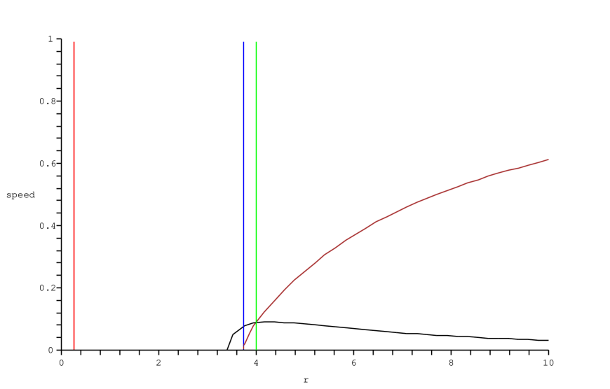
Figure 3: Illustrative graph of the speed of sound and rotational velocity of the vortex as a function of $r$. ($m=2$, $a=1$, 30’th-order Taylor series.)

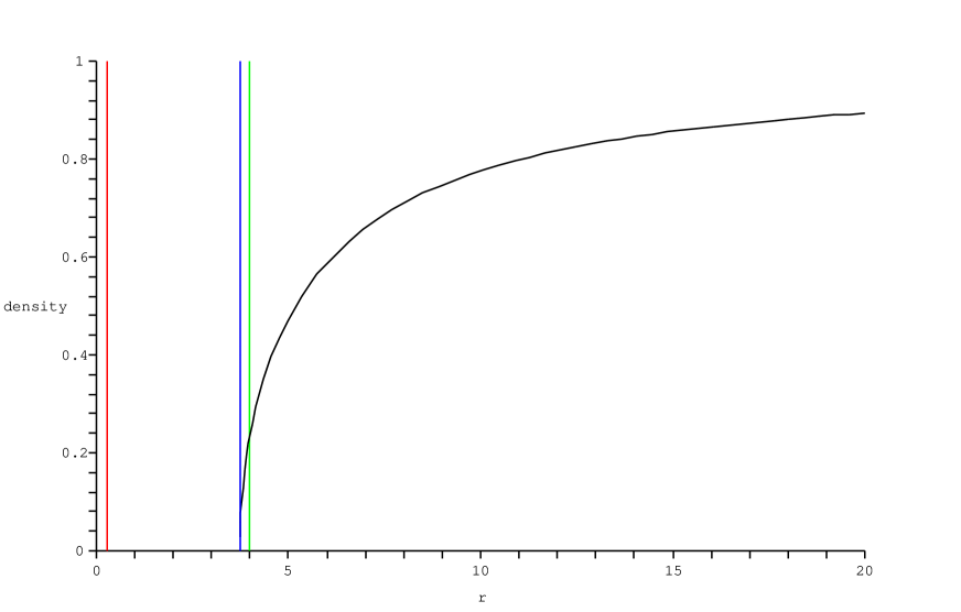
Figure 4: Illustrative graph of the fluid density as a function of $r$. ($m=2$, $a=1$, 30’th-order Taylor series.)

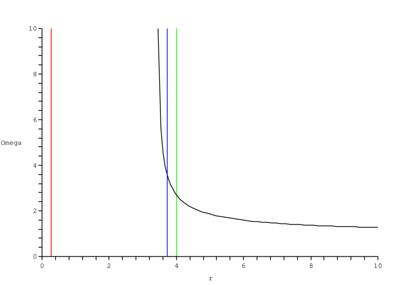
Figure 5: Illustrative graph of the conformal factor $\Omega$ as a function of $r$. ($m=2$, $a=1$, 30’th-order Taylor series.)

5 Discussion

We have shown that the Kerr equator can [in principle] be exactly simulated by an acoustic analogue based on a vortex flow with a very specific equation of state and subjected to a very specific external force. Furthermore we have as a result of the analysis also seen that such an analogue would have to be very specifically and deliberately engineered. Thus the results of this investigation are to some extent mixed, and are more useful for theoretical investigations, and for the gaining of insight into the nature of the Kerr geometry, than they are for actual laboratory construction of a vortex simulating the Kerr equator.

One of the technical surprises of the analysis was that the Doran [26, 27] coordinates (the natural generalization of the Painléve–Gullstrand coordinates that worked so well for the Schwarzschild geometry) did not lead to a useful acoustic metric even on the equator of the Kerr spacetime. Ultimately, this can be traced back to the fact that in Doran coordinates the space part of the Kerr metric is non-diagonal, even on the equator, and that no simple coordinate change can remove the off-diagonal elements. In Boyer–Lindquist coordinates however the space part of the metric is at least diagonal, and the $\tilde{r}$ coordinate introduced above makes the spatial part of the equatorial geometry conformally flat. This $\tilde{r}$ coordinate is thus closely related to the radial coordinate in the isotropic version of the Schwarzschild solution and $\tilde{r}$ in fact reduces to that isotropic radial coordinate as $a\to 0$.

However, in a more general physical setting the Doran [26, 27] coordinates might still be useful for extending the acoustic analogue away from the equator, and into the bulk of the domain of outer communication. To do this we would have to extend and modify the notion of acoustic geometry. The fact that the spatial slices of the Kerr geometry are never conformally flat [17, 18, 19] forces any attempt at extending the acoustic analogy to consider a more general class of acoustic spacetimes. A more general physical context that may prove suitable in this regard is anisotropic fluid media, and we are currently investigating this possibility. The simplest anisotropic fluid media are the classical liquid crystals [28, 29], which in the present context suffer from the defect that they possess considerable viscosity and exist chiefly at room temperature — this makes then unsuitable for the construction of analogue horizons, and particularly unsuitable for the investigation of quantum aspects of analogue horizons. Much more promising in this regard are the quantum liquid crystals. These are anisotropic superfluids such as, in particular, 3He–A [21, 30]. The anisotropic superfluids are generally characterized by the presence of a non-scalar order parameter; they behave as superfluid liquid crystals, with zero friction at $T=0$. The premier example of an anisotropic superfluid is fermionic 3He–A, where the effective gravity for fermions is described by vierbeins, though several types of Bose and Fermi condensates of cold atoms also exhibit similar behaviour [21, 30].

In the system we have presented above we have found that two of the main features of the Kerr geometry appear: the horizon (outer horizon) and ergo-region. By slight modification of standard arguments, these geometric features are expected to lead to the quantum phenomena of super-radiance and Hawking radiation [1, 2, 3, 4, 5]. The super-radiance corresponds to the reflection and amplification of a wave packet at the ergo surface [31]. (See also [32, 33].) The model, because it contains a horizon, also satisfies the basic requirements for the existence of Hawking radiation, which would now be a thermal bath of phonons emitted from the horizon [1].  These are two of the most fundamental physics reasons for being interested in analogue models [5]. A subtlety in the argument that leads to Hawking radiation arises from the way that the choice of coordinates seems to influence the choice of quantum vacuum state. In the presence of a horizon, the choice of quantum vacuum is no longer unique, and standard choices for the quantum vacuum are the Unruh, Hartle–Hawking, and Boulware states. It is the Unruh vacuum that corresponds (for either static or stationary black holes) to Hawking radiation into an otherwise empty spacetime, while the Hartle–Hawking vacuum (for a static black hole) corresponds to a black hole in thermal equilibrium with its environment (at the Hawking temperature). For a stationary [non-static] black hole the Hartle–Hawking vacuum state does not strictly speaking exist [34], but there are quasi-Hartle–Hawking quantum states that possess most of the relevant features [35]. In general relativity, because physics is coordinate independent, the choice of vacuum state is manifestly independent of the choice of coordinate system. In the analogue spacetimes considered in this article, because the preferred choice of coordinate system is intimately tied to the flowing medium, the situation is perhaps less clear. The coordinate system we have adopted is invariant under combined time reversal and parity, which might tempt one to feel that a pseudo-Hartle–Hawking vacuum is the most natural one. On the other hand, if we think of building up the vortex from a fluid that is initially at rest, then there is clearly a preferred time direction, and the “white hole” component of the maximally extended horizon would exist only as a mathematical artifact. In this physical situation the Unruh vacuum is the most natural one. We feel that there is an issue worth investigating here, to which we hope to return in some future article.

Finally, since astrophysically all black holes are expected to exhibit some degree of rotation, it is clear that an understanding of the influence of rotation on analogue models is important if one wishes to connect the analogue gravity programme back to astrophysical observations.  In conclusion, there are a number of basic physics reasons for being interested in acoustic analogues of the Kerr geometry, and a number of interesting directions in which the present analysis might be extended.

Appendix:
Isotropic version of the Schwarzschild geometry cast in acoustic form

The isotropic version of the Schwarzschild geometry can be cast exactly into acoustic form, without any extraneous conformal factors. Since this is not the standard way of viewing the acoustic analogue of the Schwarzschild geometry [4], and since the algebra is simple enough to be done in closed form, it is worthwhile taking a small detour.

In isotropic coordinates the Schwarzschild geometry reads

$${\mathrm{d}}s^{2}=-{(1-{m\over 2r})^{2}\over(1+{m\over 2r})^{2}}\;{\mathrm{d}}t^{2}+\left(1+{m\over 2r}\right)^{4}\left\{{\mathrm{d}}r^{2}+r^{2}({\mathrm{d}}\theta^{2}+\sin^{2}\theta\;{\mathrm{d}}\phi^{2})\right\},$$ (79)

and so in these coordinates the acoustic analogue corresponds to

$$v = 0;$$ (80)

$$\rho = \rho_{\infty}\;\left(1-{m^{2}\over 4r^{2}}\right);$$ (81)

$$c^{2} = c^{2}_{\infty}\;{(1-{m\over 2r})^{2}\over(1+{m\over 2r})^{6}}.$$ (82)

The external force required to hold this configuration in place against the pressure gradient is

$$f_{\hat{r}}={{\mathrm{d}}p\over{\mathrm{d}}r}=c^{2}\;{{\mathrm{d}}\rho\over{\mathrm{d}}r}=\rho_{\infty}\;c^{2}_{\infty}\;{(1-{m\over 2r})^{2}\over(1+{m\over 2r})^{6}}\;{m^{2}\over 2r^{3}}.$$ (83)

The pressure itself (normalizing $p_{\infty}\to 0$) is then

$$p(r)=-\rho_{\infty}\;c^{2}_{\infty}\;m^{2}\;\left({120r^{3}-20r^{2}m+10m^{2}r+m^{3}\over 480\;r^{5}\;(1+{m\over 2r})^{5}}\right),$$ (84)

and by eliminating $r$ in favour of $\rho$ using

$$r={m\over 2\sqrt{1-\rho/\rho_{\infty}}}$$ (85)

we can deduce the equation of state

$$p(\rho)=-(\rho_{\infty}-\rho)\;c^{2}_{\infty}\;\left({20-5\rho/\rho_{\infty}-4\sqrt{1-\rho/\rho_{\infty}}-\rho/\rho_{\infty}\sqrt{1-\rho/\rho_{\infty}}\over 15\;(1+\sqrt{1-\rho/\rho_{\infty}})^{5}}\right).$$ (86)

At the horizon, which occurs at $r_{H}=m/2$ in these coordinates, both $\rho=0$ and $c=0$ in the acoustic analogue, while

$$p_{H}=-{\rho_{\infty}\;c^{2}_{\infty}\over 30}$$ (87)

is finite, so there is a finite pressure drop between asymptotic infinity and the horizon. Everything is now simple enough to be fully explicit, and although we now have an analogue model that reproduces the exterior part of the Schwarzschild geometry exactly, we can also clearly see the two forms in which fine tuning arises — in specifying the external force, and in the equation of state.

More generally, it is a standard result that any spherically symmetric geometry can be put into isotropic form

$${\mathrm{d}}s^{2}=-\exp[-2\Phi]\;{\mathrm{d}}t^{2}+\exp[-2\Psi]\left\{{\mathrm{d}}r^{2}+r^{2}({\mathrm{d}}\theta^{2}+\sin^{2}\theta\;{\mathrm{d}}\phi^{2})\right\}.$$ (88)

This can be put into acoustic form in a particularly simple manner by setting

$$v(r) = 0;$$ (89)

$$\rho(r) = \rho_{\infty}\;\exp[-\Phi-\Psi];$$ (90)

$$c(r) = c_{\infty}\;\exp[\Psi-\Phi].$$ (91)

The pressure can now be formally evaluated as

$$p(r)=\rho_{\infty}\;c_{\infty}^{2}\int_{r}^{\infty}\exp[\Psi-3\Phi]\;\partial_{r}(\Phi+\Psi)\;{\mathrm{d}}r,$$ (92)

and comparison with $\rho(r)$ can be used to construct a formal equation of state, $\rho(p)$.

References

References

- [1] W. G. Unruh, “Experimental Black Hole Evaporation,” Phys. Rev. Lett. 46 (1981) 1351.
- [2] W. G. Unruh, “Sonic analog of black holes and the effects of high frequencies on black hole evaporation,” Phys. Rev. D 51 (1995) 2827 [arXiv:gr-qc/9409008].
- [3] M. Visser, “Acoustic Propagation In Fluids: An Unexpected Example Of Lorentzian Geometry,” arXiv:gr-qc/9311028.
- [4] M. Visser, “Acoustic black holes: Horizons, ergospheres, and Hawking radiation,” Class. Quant. Grav. 15 (1998) 1767 [arXiv:gr-qc/9712010].
- [5] M. Novello, M. Visser and G. Volovik, “Artificial Black Holes”, (World Scientific, Singapore, 2002).
- [6] Carlos Barcelo, Stefano Liberati, Sebastiano Sonego, and Matt Visser, “Causal structure of acoustic spacetimes”, arXiv:gr-qc/0408022.
- [7] S. E. Perez Bergliaffa, K. Hibberd, M. Stone and M. Visser, “Wave Equation for Sound in Fluids with Vorticity,” Physica D191 (2004) 121–136 [arXiv:cond-mat/0106255].
- [8] T. Jacobson and G. Kang, “Conformal Invariance Of Black Hole Temperature,” Class. Quant. Grav. 10 (1993) L201 [arXiv:gr-qc/9307002].
- [9] C. Barcelo, S. Liberati and M. Visser, “Analogue models for FRW cosmologies,” Int. J. Mod. Phys. D 12 (2003) 1641 [arXiv:gr-qc/0305061].
- [10] C. Barcelo, S. Liberati and M. Visser, “Probing semiclassical analogue gravity in Bose–Einstein condensates with widely tunable interactions,” Phys. Rev. A 68 (2003) 053613 [arXiv:cond-mat/0307491].
- [11] P. O. Fedichev and U. R. Fischer, “’Cosmological’ particle production in oscillating ultracold Bose gases: The role of dimensionality,” Phys. Rev. A 69, 033602 (2004) [arXiv:cond-mat/0303063].
- [12] P. O. Fedichev and U. R. Fischer, “Hawking radiation from sonic de Sitter horizons in expanding Bose-Einstein-condensed gases,” Phys. Rev. Lett. 91 (2003) 240407 [arXiv:cond-mat/0304342].
- [13] P. O. Fedichev and U. R. Fischer, “Observing quantum radiation from acoustic horizons in linearly expanding cigar-shaped Bose-Einstein condensates,” Phys. Rev. D 69 (2004) 064021 [arXiv:cond-mat/0307200].
- [14] J. E. Lidsey, “Cosmic dynamics of Bose-Einstein condensates,” Class. Quant. Grav. 21 (2004) 777 [arXiv:gr-qc/0307037].
- [15] S. E. Ch. Weinfurtner, “Simulation of gravitational objects in Bose–Einstein condensates. (In German),” arXiv:gr-qc/0404022.
- [16] S. E. Ch. Weinfurtner, “Analog model for an expanding universe,” arXiv:gr-qc/0404063.
- [17] A. Garat and R. H. Price, “Nonexistence of conformally flat slices of the Kerr spacetime”, Phys. Rev. D 61 (2000) 124011 [arXiv:gr-qc/0002013].
- [18] J. A. Valiente Kroon, “On the nonexistence of conformally flat slices in the Kerr and other stationary spacetimes,” arXiv:gr-qc/0310048;
- [19] J. A. Valiente Kroon, “Asymptotic expansions of the Cotton-York tensor on slices of stationary spacetimes,” Class. Quant. Grav. 21 (2004) 3237 [arXiv:gr-qc/0402033].
- [20] R. M. Wald, “General Relativity,” (University of Chicago Press,1984).
- [21] G. Volovik, “The universe in a Helium droplet”, (Oxford University Press, 2003).
- [22] R. P. Kerr, “Gravitational field of a spinning mass as an example of algebraically special metrics,” Phys. Rev. Lett. 11 (1963) 237.
- [23] R. H. Boyer and R. W. Lindquist, “Maximal analytic extension of the Kerr metric,” J. Math. Phys. 8 (1967) 265.
- [24] T. A. Jacobson and G. E. Volovik, “Effective spacetime and Hawking radiation from moving domain wall in thin film of He-3-A,” Pisma Zh. Eksp. Teor. Fiz. 68, 833–838 (1998) [JETP Lett. 68, 874–880 (1998)] [arXiv:gr-qc/9811014].
- [25] T. Jacobson and T. Koike, “Black hole and baby universe in a thin film of He-3-A”. Published in Artificial Black Holes Ed. M. Novello, M. Visser and G. Volovik, (World Scientific, Singapore, 2002) [arXiv:cond-mat/0205174].
- [26] C. Doran, “A new form of the Kerr solution,” Phys. Rev. D 61 (2000) 067503 [arXiv:gr-qc/9910099].
- [27] A. J. S. Hamilton and J. P. Lisle, “The river model of black holes,” arXiv:gr-qc/0411060.
- [28] S. Chandrasekhar, “Liquid crystals”, (Cambridge University Press, 1992).
- [29] P. J. Collings and M. Hird, “Introduction to liquid crystals”, (Taylor and Francis, London, 2004).
- [30] G. E. Volovik, “Superfluid analogies of cosmological phenomena,” Phys. Rept. 351 (2001) 195 [arXiv:gr-qc/0005091].
- [31] T. R. Slatyer and C. M. Savage, “Superradiant scattering from a hydrodynamic vortex”, unpublished.
- [32] S. Basak and P. Majumdar, “‘Superresonance’ from a rotating acoustic black hole,” Class. Quant. Grav. 20 (2003) 3907 [arXiv:gr-qc/0203059].
- [33] S. Basak and P. Majumdar, “Reflection coefficient for superresonant scattering,” Class. Quant. Grav. 20 (2003) 2929 [arXiv:gr-qc/0303012].
- [34] R. M. Wald, “The thermodynamics of black holes,” Living Rev. Rel. 4 (2001) 6 [arXiv:gr-qc/9912119].
- [35] B. R. Iyer and A. Kumar, “The Kerr black hole in thermal equilibrium and the -vacuum”, J. Phys. A: Math. Gen. 12 (1979) 1795–1803.
- [36] T. K. Das, “Analogue Hawking radiation from astrophysical black hole accretion,” Class. Quant. Grav. 21 (2004) 5253 [arXiv:gr-qc/0408081].
- [37] T. K. Das, “Transonic Black Hole Accretion as Analogue System,” arXiv:gr-qc/0411006.