Asymptotic quasinormal modes of a coupled scalar field in the Garfinkle-Horowitz-Strominger dilaton spacetime

Abstract

The analytic forms of the asymptotic quasinormal frequencies of a coupled scalar field in the Garfinkle-Horowitz-Strominger dilaton spacetime is investigated by using the monodromy technique proposed by Motl and Neitzke. It is found that the asymptotic quasinormal frequencies depend not only on the structure parameters of the background spacetime, but also on the coupling between the scalar fields and gravitational field. Moreover, our results show that only in the minimal couple case, i.e., $\xi$ tends zero, the real parts of the asymptotic quasinormal frequencies agrees with the Hod’s conjecture, $T_{H}\ln{3}$.

I Introduction

It is well known that quasinormal modes possess a discrete spectra of complex characteristic frequencies which are entirely fixed by the structure of the background spacetime and are irrelevant of the initial perturbationsChandrasekhar . Thus, one can directly identify a black hole existence through comparing the quasinormal modes with the gravitational waves observed in the universe. Meanwhile, it is generally believed that the study of the quasinormal modes may lead to a deeper understanding of black holes and quantum gravity because that the quasinormal frequency spectra is related to the AdS/CFT correspondence, string theory and loop quantum gravityHod98 -Zerilli70 . Therefore, much attention has been devoted to the study of the quasinormal modes in the recent thirty yearsDetweiler -Bachelot . In the Schwarzschild spacetime, one found that the asymptotic quasinormal frequencies of high overtones are described by

$$\frac{2\pi\omega}{\kappa}=\ln{3}+i(2n+1)\pi,\ \ \ n\rightarrow\infty,$$ (1)

where $\kappa$ is the surface gravity constant of the black hole. Formula (1) was derived numericallyNollert and subsequently confirmed analyticallyAndersson Motl03 .

HodHod98 first conjectured that the real parts of the asymptotic quasinormal frequencies of a Schwarzschild black hole can be expressed as $\omega_{R}=T_{H}\ln{3}$. Together with Bohr’s correspondence principle, the first law of black hole thermodynamics and the asymptotic quasinormal modes, he also obtained some new information about the quantization of area at a black hole event horizon. Using of Hod’s conjecture, DreyerDreyer03 found that the quasinormal modes can entirely fixed the Barbero-Immirzi parameterImmirzi57 , which was introduced as an indefinite factor by Immirzi to obtain the right form of the black hole entropy in the loop quantum gravity. Most significantly, the presence of $\ln{3}$ also means that the gauge group in the loop quantum gravity should be $SO(3)$ rather than $SU(2)$. Thus, one suggested that Hod’s conjecture maybe create a new way to probe the quantum properties of black hole.

However, the question whether Hod’s conjecture applies to more general black holes still remain open. Recently, we probed the asymptotic quasinormal modes of a massless scalar field in the Garfinkle-Horowitz-Strominger dilaton spacetime04 and find that the frequency spectra formula satisfies Hod’s conjecture. Cardoso and Abdalla Cardoso Abdalla found the asymptotic quasinormal frequencies in the Schwarzschild de Sitter and Anti-de Sitter spacetimes depend on the cosmological constant. Only under the condition that the cosmological constant vanishes, the real parts of the asymptotic quasinormal frequencies returns to $T_{H}\ln{3}$. For the Reissner-Nordström black hole, L. Motl and A.NeitzkeMotl03 obtained the asymptotic quasinormal frequencies is relevant of the electric charge $Q$. It is unfortunately that the asymptotic quasinormal frequencies do not return returns $T_{H}\ln{3}$ as the black hole charge $Q$ tends to zero. Thus, some authorsBerti suggested that Hod’s conjecture should be modified in some way. However, how does the correct modification look like? It is an interesting subject need to be study more deeply in the future. At present, it is necessary and important to study the asymptotic quasinormal modes in the more general background spacetimes.

In this paper, our main purpose is to investigate the asymptotic quasinormal modes of a coupled scalar field in the Garfinkle-Horowitz-Strominger dilaton spacetime. We find that besides dependence on the structure parameters of the background spacetime, the asymptotic quasinormal frequencies also are relevant of the couple constant $\xi$. The plan of the paper is as follows. In Sec.II, we derive analytically the asymptotic quasinormal frequency formula of a coupled scalar field in the Garfinkle-Horowitz-Strominger dilaton spacetime by making use of the monodromy methodMotl03 . At the last, a summary and some discussions are presented.

II Asymptotic quasinormal frequencies formula of a coupled scalar field in the Garfinkle-Horowitz-Strominger dilaton spacetime

In standard coordinates, the metric for the Garfinkle-Horowitz-Strominger dilaton black hole spacetime can be expressed as Garfinkle91

$$ds^{2}=-\left(1-\frac{2M}{r^{\prime}}\right)dt^{2}+\left(1-\frac{2M}{r^{\prime}}\right)^{-1}dr^{2}+r^{\prime}(r^{\prime}-2a)d\Omega^{2},$$ (2)

$$e^{-2\phi} = e^{-2\phi_{0}}\left(1-\frac{2a}{r^{\prime}}\right),$$

where $M$ represents the black hole mass and $a$ is a parameter related to dilaton field. The dilaton field is given by $e^{-2\phi}=e^{-2\phi_{0}}(1-\frac{Q^{2}}{Mr^{\prime}})$, where $\phi_{0}$ is the dilaton value at $r^{\prime}\rightarrow\infty$ and $Q$ is the electric charge carried by this black hole. The relationship among mass $M$, the charge $Q$ and $a$ is described as $a=\frac{Q^{2}}{2M}$. This black hole has an event horizon at $r^{\prime}=2M$ and two singular points at $r^{\prime}=0$ and $r^{\prime}=2a$. The Hawking temperature $T_{H}=\frac{1}{8\pi M}$ is the same as that of the Schwarzschild spacetime.

In order to simplify the calculation, we introduce a coordinate change

$$r=\sqrt{r^{\prime}(r^{\prime}-2a)}.$$ (3)

Then the metric (2) can be rewritten as

$$ds^{2}=-\left(1-\frac{2M}{a+\sqrt{a^{2}+r^{2}}}\right)dt^{2}+\left(1-\frac{2M}{a+\sqrt{a^{2}+r^{2}}}\right)^{-1}\frac{r^{2}}{r^{2}+a^{2}}dr^{2}+r^{2}d\Omega^{2}.$$ (4)

The event horizon of the black hole is now located at $r=2\sqrt{M(M-a)}$ and the Hawking temperature is still described by $T_{H}=\frac{1}{8\pi M}$. By means of the quantity $R_{\alpha\beta\gamma\delta}R^{\alpha\beta\gamma\delta}$, we find that the point $r=0$ is a curvature singular point.

The general perturbation equation for a coupled massless scalar field in the dilaton spacetime is given by Frolov

$$\frac{1}{\sqrt{-g}}\partial_{\mu}(\sqrt{-g}g^{\mu\nu}\partial_{\nu})\psi-\xi R\psi=0,$$ (5)

where $\psi$ is the scalar field and $R$ is the Ricci scalar curvature. The coupling between the scalar field and the gravitational field represented by the term $\xi R\psi$, where $\xi$ is a numerical couple factor.

After adopting WKB approximation $\psi=\frac{e^{-i\omega t}\phi(r)}{r}Y(\theta,\varphi)$, introducing a tortoise coordinate

$$x=\sqrt{a^{2}+r^{2}}-a+2M\ln{\left[\frac{\sqrt{a^{2}+r^{2}}-(2M-a)}{2(M-a)}\right]},$$ (6)

and substituting Eqs.(4) and (6) into Eq.(5), we know that the radial perturbation equation for a coupled scalar field in the Garfinkle-Horowitz-Strominger dilaton spacetime can be expressed as

$$\frac{d^{2}\phi}{dx^{2}}+(\omega^{2}-V[r(x)])\phi=0,$$ (7)

where

$$V[r(x)] = \left(1-\frac{2M}{a+\sqrt{a^{2}+r^{2}}}\right)\times$$ (8)

$$\left[\frac{l(l+1)}{r^{2}}+\frac{2M(a^{2}+r^{2})^{3/2}-2\sqrt{a^{2}+r^{2}}a^{3}+2Ma^{3}-2a^{4}-r^{2}a^{2}}{r^{4}(a+\sqrt{r^{2}+a^{2}})^{2}}+\xi R\right],$$

and

$$R=\frac{2a^{2}(r^{2}+2aM-2M\sqrt{a^{2}+r^{2}})}{r^{6}}.$$ (9)

It is well known that the quasinormal modes consist of the solutions of the perturbation equation (7) with the boundary conditions appropriate for purely ingoing waves at the event horizon and purely outgoing waves at infinity, namely,

$$\phi = e^{+i\omega x},\ \ \ \ \ \ x\rightarrow-\infty,$$

$$\phi = e^{-i\omega x},\ \ \ \ \ \ x\rightarrow+\infty.$$ (10)

In general, we just consider the perturbation equation (7) in the physical region $r\geq 2\sqrt{M(M-a)}$ in the Garfinkle-Horowitz-Strominger dilaton black hole. However, in the monodromy method, it is fundamental to extend analytically Eq.(7) to the whole complex $r$-plane. In the process of analytical extension, we find that both the tortoise coordinate $x(r)$ and the wave function $\phi(r)$ are multivalued around the singular points $r=0$ and $r=2\sqrt{M(M-a)}$ . This multivaluedness plays an important and essential role in our analysis. As in Ref.Motl03 , we can put branch cuts in the complex $r$-plane from $r=0$ to $r=2\sqrt{M(M-a)}$ in order to avoid dealing with multivalued functions. The monodromy of $\phi(r)$ can be defined by the discontinuity across the cut. Finally, by comparing the local and global monodromy of $\phi(r)$ along the selected contour $L$ around the point $r=2\sqrt{M(M-a)}$, we can obtain the asymptotic quasinormal frequency spectra in the Garfinkle-Horowitz-Strominger dilaton black hole spacetime.

From Eq.(6), we find that $x$ is not uniquely defined as a function of $r$. However, it is very fortunate that we can determine the sign of $Re(x)$ in the complex $r$-plane. The regions for the different sign of $Re(x)$ are shown in the Figure 1.

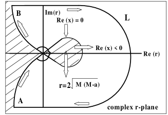
Figure 1: The complex $r$-plane and the contour $L$. The regions with the hachures denote the area $Re(x)<0$.

As in Ref.Motl03 , in order to compute conveniently, we may introduce the variable $z=x-\frac{\pi i}{2\kappa}$. For $r=0$, we have $z=0$. To fix the angle of the variable $z$ at the point $r=0$, we define the branch $n=0$ for $\ln{(-1)}$.

Now, we must define the boundary condition at $r=\infty$. Similarly to Ref.Motl03 , we can analytically continue $\phi(r)$ via “Wick rotation” to the line $Im(\omega x)=0$. For the highly damped modes, i.e., $\omega$ are almost purely imaginary, the line $Im(\omega x)=0$ is just slightly sloped off the line $Re(x)=0$. Assuming initially that $Re(\omega)>0$ and then making use of the condition $Im(\omega x)=0$, we can obtain $x=+\infty$ is rotated to $\omega x=+\infty$. Thus, on the line $Re(x)=0$, the boundary condition at $r=+\infty$ actually becomes

$$\phi(r)\sim e^{-i\omega x},\ \ \ \ \omega x\rightarrow+\infty.$$ (11)

Let us now compute the local monodromy around the singular point $r=2\sqrt{M(M-a)}$. This can be done by matching the asymptotic along the line $Re(x)=0$, i.e., the contour $L$ shown in the Fig. 1. When we start at point $A$ and move along the contour $L$ towards interior, the $\phi(x)$ can be look as the plane waves because the term $\omega^{2}$ dominates the potential in Eq.(7) away from the origin point. At the vicinity of the point $r=0$, we have

$$z\sim-\frac{r^{2}}{2(M-a)},$$ (12)

and the behaviors of the Ricci scalar curvature and the potential are

$$R\sim\frac{2a(a-M)}{r^{4}},$$ (13)

and

$$V[r(z)]\sim-\frac{1-2\xi}{4z^{2}}.$$ (14)

We make the identification $j=\sqrt{2\xi}$, and then the perturbation equation (7) can be rewritten as

$$(\frac{d^{2}}{dz^{2}}+\omega^{2}+\frac{1-j^{2}}{4z^{2}})\phi(z)=0.$$ (15)

From the Ref.handbook , we find it can be exactly solved in terms of the Bessel function and the general solution near the origin point can be expressed as

$$\phi(z)=A_{+}c_{+}\sqrt{\omega z}J_{+j/2}(\omega z)+A_{-}c_{-}\sqrt{\omega z}J_{-j/2}(\omega z).$$ (16)

Now, let us look for the asymptotic forms of the solution (16) away from the origin. After considering the asymptotic behavior of $J_{\pm j/2}(\omega z)$ as $\omega z\rightarrow\infty$, we can select the normalization factors $c_{\pm}$ in (16) so that we can write the asymptotic forms as

$$c_{\pm}\sqrt{\omega z}J_{\pm\frac{j}{2}}(\omega z)\sim 2\cos{(\omega z-\alpha_{\pm})},$$ (17)

as $\omega z\rightarrow\infty$ , where $\alpha_{\pm}=\frac{\pi}{4}(1\pm j)$. From Eqs.(16), (17) and the boundary condition (11), we have

$$A_{+}e^{-i\alpha_{+}}+A_{-}e^{-i\alpha_{-}}=0,$$ (18)

and

$$\phi(z)\sim(A_{+}e^{i\alpha_{+}}+A_{-}e^{i\alpha_{-}})e^{-i\omega z}.$$ (19)

To follow the contour $L$ and approach to the point $B$, we have to turn an angle $\frac{3\pi}{2}$ around the origin $r=0$, corresponding to $3\pi$ around $z=0$. From the Bessel function behavior near the origin point

$$J_{\pm\frac{j}{2}}(\omega z)=z^{\pm\frac{j}{2}}\varphi(z),$$ (20)

where $\varphi(z)$ is an even holomorphic function, we find that after the $3\pi$ rotation the asymptotic are

$$c_{\pm}\sqrt{\omega z}J_{\pm\frac{j}{2}}(\omega z)\sim e^{6i\alpha_{\pm}}2\cos{(-\omega z-\alpha_{\pm})},$$ (21)

as $\omega z\rightarrow-\infty$. Thus the asymptotic at the point $B$

$$\phi(z)\sim(A_{+}e^{5i\alpha_{+}}+A_{-}e^{5i\alpha_{-}})e^{-i\omega z}+(A_{+}e^{7i\alpha_{+}}+A_{-}e^{7i\alpha_{-}})e^{i\omega z},\ \ \ \ \omega z\rightarrow-\infty.$$ (22)

Finally, we can come back from the point $B$ to the point $A$ along the large semicircle in the right half-plane. In this region, because the term $\omega^{2}$ dominates the potential $V[r(x)]$, we can approximate the solutions of the perturbation equation as plane waves. When we return to the point $A$, the coefficient of $e^{-i\omega z}$ remains unchange. While the coefficient of $e^{i\omega z}$ makes only an exponentially small contribution to $\phi(z)$ in the right plane. Finally, we find that the monodromy around the contour $L$ must multiply the coefficient of $e^{-i\omega z}$ by a factor

$$\frac{A_{+}e^{5i\alpha_{+}}+A_{-}e^{5i\alpha_{-}}}{A_{+}e^{i\alpha_{+}}+A_{-}e^{i\alpha_{-}}}=\frac{e^{6i\alpha_{+}}-e^{6i\alpha_{-}}}{e^{2i\alpha_{+}}-e^{2i\alpha_{-}}}=-(1+2\cos{\pi j}).$$ (23)

Now, let us calculate the global monodromy around the contour $L$. Since the only singularity of $\phi(r)$ or $e^{-i\omega z}$ inside the contour occurs at the point $r=2\sqrt{M(M-a)}$, according to the boundary condition of the quasinormal modes, we can obtain the monodromy of $\phi(r)$ or $e^{-i\omega z}$ at this point. After a full clockwise round trip, $\phi(r)$ acquires a phase $e^{\frac{\pi\omega}{\kappa}}$, while $e^{-i\omega z}$ acquires a phase $e^{-\frac{\pi\omega}{\kappa}}$. So the coefficient of $e^{-i\omega z}$ in the asymptotic of $\phi(r)$ must be multiplied by $e^{\frac{2\pi\omega}{\kappa}}$. Substituting $j=\sqrt{2\xi}$ into Eq.(23) and comparing the local monodromy with the global one, we find the asymptotic quasinormal frequencies of a coupled scalar field in the Garfinkle-Horowitz-Strominger dilaton black hole spacetime satisfy

$$e^{\frac{2\pi\omega}{\kappa}}=-[1+2\cos{(\sqrt{2\xi}\pi)}].$$ (24)

Making a simple operation on Eq.(24), we obtain easily the formula

$$\frac{2\pi\omega}{\kappa}=\ln{[1+2\cos{(\sqrt{2\xi}\pi)}]}+i(2n+1)\pi,\ \ \ \ n\rightarrow\infty.$$ (25)

It is interesting to note that the right-hand side of the formula (25) contains the couple factor $\xi$. This means that the asymptotic quasinormal modes depend not only on the structure parameters of the background spacetimes, but also on the coupling between the matter fields and gravitational field. Furthermore, we find only when $\xi=0$, namely, in the minimal couple case, the real part of the right-hand side of the formula (25) becomes $\ln{3}$, which is consistent with Hod’s conjecture.

III Summary and discussion

We have investigated the analytical forms of the asymptotic quasinormal frequencies for a coupled scalar field in the Garfinkle-Horowitz-Strominger dilaton spacetime by adopting the monodromy technique. It is shown that the asymptotic quasinormal frequencies depend not only on the structure parameters of the background spacetime, but also on a couple constant $\xi$. The fact tells us that the interaction between the matter fields and gravitational field will affect the frequencies spectra formula of the asymptotic quasinormal modes. It is a novel property of the quasinormal modes in Garfinkle-Horowitz-Strominger dilaton spacetime. In the Schwarzschild and Reissner-Nordström spacetimes, we find the asymptotic quasinormal frequencies do not possess this behavior because the curvature scalar $R$ in both the spacetimes is equal to zero and then the coupled term in Eq.(5) vanishes. Moreover, we find that Hod’s conjecture, the real parts of the asymptotic quasinormal frequencies equals to $T_{H}\ln{3}$, is valid only for the minimal couple case in the Garfinkle-Horowitz-Strominger dilaton spacetime, i.e., $\xi$ becomes zero. It implies that there maybe exist a more general form of the Hod’s conjecture.

It should be pointed out that although the formula (25) is not related to the dilaton field parameter $a$ obviously, it does not means that the quasinormal modes are independent of the dilaton. The reason is that we just consider the contribution of the leading term $r^{-4}$ in the potential $V$ to the local monodromy of the wave function $\phi(z)$. If we consider the contribution of the lower order terms in the potential $V(r)$, the corrected term to the asymptotic quasinormal frequencies will depend on the parameter $a$ of the dilaton field. For example, as $a$ is very small, the main corrected term is roughly in proportion to $\frac{(1-i)}{\sqrt{n+1/2}}[l(l+1)+1-\frac{2M}{3(M+a)}]$, which shows that the quasinormal frequencies increase as $a$ increases in the Garfinkle-Horowitz-Strominger dilaton spacetime.

- (1) S. Chandrasekhar and S. L. Detweiler, Proc. R. Soc. London A 344, 441 (1975).
- (2) S. Hod, Phy. Rev. Lett. 81, 4293 (1998).
- (3) O. Dreyer, Phy. Rev. Lett. 90, 081301 (2003).
- (4) G. Immirzi, Nucl. Phys. Proc. Suppl. 57, 65 (1997).
- (5) B. Wang , C. Y. Lin and E. Abdalla, Phys. Lett. B 481, 79 (2000).
- (6) J. Maldacena, Adv. Theor. Math. Phys. 2, 253 (1998).
- (7) T. Regge and J. A. Wheeler, Phys. Rev. 108, 1063 (1957).
- (8) F. J. Zerilli, Phys.Rev. Lett. 24, 737 (1970).
- (9) S. L. Detweiler and E. Szedenits, Astrophys. J. 231, 211 (1979).
- (10) S. L. Smarr, Sources of Gravitational Radiation (Cambridge University Press, 1979).
- (11) E. W. Leaver, Proc. R. Soc. A 402, 285 (1985).
- (12) H. P. Nollert, Phy. Rev. D 47, 5253 (1993).
- (13) N. Andersson, Class. Quantum Grav. 10, L61 (1993).
- (14) L. Motl and A. Neitzke, Adv. Theor. Math. Phys. 7, 307 (2003).
- (15) A. Corichi, Phys. Rev. D 67 , 087502 (2003).
- (16) A. C. Martinez, R. Troncoso and J. Zanelli, Phys. Rev. D 67, 087104 (2002).
- (17) L. Motl, Adv. Theor. Math. Phys. 6, 1135 (2003).
- (18) G. Kunstatter, Phys. Rev. Lett. 90, 161301 (2003).
- (19) D. Birmingham Phys. Rev. D 64, 064024 (2001).
- (20) D. Birmingham, I. Sachs and S. N. Solodukhin, Phys. Rev. Lett. 88, 151301 (2002).
- (21) V. Cardoso and J. P. S. Lemos, Phys. Rev.D 63, 124015 (2001).
- (22) M. Giammatteo and J. L. Jing, gr-qc/0403030.
- (23) J. L. Jing, Phys. Rev. D 69, 084009 (2004).
- (24) R. A. Konoplya, Phys. Rev. D 68, 024018 (2002).
- (25) A. Bachelot, Annales Poincare Phys. Theor. 59, 3 (1993).
- (26) S. B. Chen and J. L. Jing, Chin. Phys. Lett., to be published.
- (27) V. Cardoso, J. Natario and R. Schiappa, hep-th/0403132.
- (28) K. H. C. Branco and E. Abdalla, gr-qc/0309090.
- (29) E. Berti, V. Cardoso, K. D. Kokkotas and H. Onozawa, Phys. Rev. D 68, 124018 (2003).
- (30) D. Garfinkle, G. T. Horowitz and A. Strominger, Phys. Rev. D 43, 3140 (1991).
- (31) V. Frolov and A. Zelnikov, Phys. Rev. D 63, 125026 (2001).
- (32) M. Abramowitz and I. A. Stegun, Handbook of Mathematical Functions (New York: Dover 1970).