Geophysical studies with laser-beam detectors of gravitational waves

Abstract

The existing high technology laser-beam detectors of gravitational waves may find very useful applications in an unexpected area - geophysics. To make possible the detection of weak gravitational waves in the region of high frequencies of astrophysical interest, $\sim 30-10^{3}~{}Hz$, control systems of laser interferometers must permanently monitor, record and compensate much larger external interventions that take place in the region of low frequencies of geophysical interest, $\sim 10^{-5}-3\times~{}10^{-3}~{}Hz$. Such phenomena as tidal perturbations of land and gravity, normal mode oscillations of Earth, oscillations of the inner core of Earth, etc. will inevitably affect the performance of the interferometers and, therefore, the information about them will be stored in the data of control systems. We specifically identify the low-frequency information contained in distances between the interferometer mirrors (deformation of Earth) and angles between the mirrors’ suspensions (deviations of local gravity vectors and plumb lines). We show that the access to the angular information may require some modest amendments to the optical scheme of the interferometers, and we suggest the ways of doing that. The detailed evaluation of environmental and instrumental noises indicates that they will not prevent, even if only marginally, the detection of interesting geophysical phenomena. Gravitational-wave instruments seem to be capable of reaching, as a by-product of their continuous operation, very ambitious geophysical goals, such as observation of the Earth’s inner core oscillations.

1 Introduction

Laser-beam detectors of gravitational waves are designed to explore the Universe in a new type of radiation and from a new perspective. With the already operating instruments, and coming soon online, we are expecting to witness the discovery of fascinating physics involved in powerful sources of cosmic gravitational radiation. The astrophysical aims of the gravitational wave (g.w.) science are well understood and comprehensively described in the literature (for recent reviews, see for example [1, 2, 3, 4]). Naturally, g.w. community is focused on the ambitious target of ‘reaching for the black holes’. But what about a more modest goal of looking inside our own planet ? No doubt, black holes are fascinating and scientifically important objects. But it is also necessary to remember that, say, the still poorly understood and unpredictable earthquakes are claiming thousands of human lives per year. Is it possible that the cutting-edge technology of g.w. interferometers [5, 6, 7, 8] may help us with accurate geophysical studies, as a by-product of the continuous search for astrophysical gravitational waves ?

This is the major question of the present work, and the answer is positive. We shall show in this paper that a laser-beam detector of gravitational waves is in fact automatically a valuable geophysical device. Without collecting, recording and processing environmental information of geophysical origin, a g.w. laser interferometer would simply be incapable of working as a sensitive astrophysical instrument. Certainly, we have to make sure that the extraction of geophysical information does not compromise the astrophysical aims of the instrument.

A laser-beam detector of gravitational waves is a conceptually simple installation. Each arm of the interferometer, typically of the length $L=3~{}km$, consists of two mirrors, and the distance variation between the mirrors is monitored by the laser beam. The mirrors are hanging on wires in supporting towers. Each mirror is essentially a mass element of the pendulum placed in the local gravitational field of the Earth. The eigen-frequency of the pendulum is normally in the range of $0.1-1~{}Hz$. The multi-stage pendulum system shields the mirrors from large uncontrollable displacements of the tops of the supporting towers. This makes the interferometer capable of measuring, in the region of relatively high frequencies of astrophysical interest $\sim 30-10^{3}~{}Hz$, the incredibly small variations of distance between the mirrors, at the level of $10^{-16}~{}cm$. The expected cause of these variations is the incoming astrophysical gravitational wave.

The isolation from noises in the region of relatively high frequencies is only a part of the story. To ensure successful performance of the interferometer as an astrophysical instrument, control systems of the interferometer should also register and compensate for large external interventions of geophysical origin that take place in the region of relatively low frequencies. For example, the tidal half-daily variations of distance beween towers separated by $3~{}km$ are typically at the level of $10^{-2}~{}cm$. This change of distance is 14 orders of magnitude larger than the anticipated astrophysical signal. If this sort of variations were allowed to affect distance between the mirrors, the interferometer would not be in the ‘locked’ state, and hence it would not be able to operate as astrophysical instrument. The ‘locking’ of the interferometer requires that the distance between the mirrors is maintained unchanged with accuracy of approximately one hundredth of the laser light wavelength, which amounts to $10^{-6}~{}cm$ and less. This means that the low-frequency variations of distance between the mirrors should be monitored and largely removed by a control system called the adjustment system. A similar monitoring and compensation should be done with respect to low-frequency variations of the angle between the interferometer mirrors. This is being done by a control system called the alighnment system. Ideally, in order to reach the astrophysical goals, control systems should keep the interferometer in the working condition for the duration of time exceeding many months.

Thus, the collected and recorded low-frequency information, which is vital for maintaining the operational state of the laser-beam detector of gravitational waves, inevitably makes the g.w. detector also a geophysical instrument. The time-scales of geophysical processes, some of which are believed to be crucial for global geodynamics, lie in the range from several minutes to several hours. In other words, we will be interested in frequencies, which we call geophysical frequencies, somewhere in the interval $10^{-5}-3\times 10^{-3}~{}Hz$.

In Sec.2 we consider a simple model of g.w. interferometer as a geophysical instrument. It is assumed that the mirrors’ suspension points can move and the plumb lines of hanging mirrors can vary. These changes arise as a result of the Earth surface deformations and variations of local gravitational field caused, for example, by the internal Earth dynamics. We derive general formulas for the distance between the mirrors and the angles between the local plumb lines. Ideally, these are two variables that are supposed to be monitored by, respectively, the adjustment and alignment systems of the interferometer.

In Sec.3 we consider a number of interesting geophysical phenomena which inevitably affect the performance of a g.w. interferometer. The signatures of these phenomena are contained in the outcomes of the adjustment and alignment control systems. The geophysical effects to be studied include tidal perturbations, normal modes of Earth oscillations, movements of the inner solid core of Earth, etc. We place the main emphasis on the fascinating phenomenon of the inner core oscillations. We estimate the useful geophysical signal accompanying this phenomenon, which will manifest itself in the variation of distance between the mirrors and in the variation of angle between the plumb lines of the hanging mirrors. The guidance for the expected amplitude of the signal is provided by the reported in the literature indications that the inner core oscillations have been actually detected by other, traditional, methods. From the requirement that the signal to noise ratio should be larger than 1, we define the level of tolerable noise in the proposed measurements. Specifically, the tolerable noise allows the detection of the useful signal, if the observation time exceeds 70, or so, inner core oscillation periods.

A useful signal can be detected if the environmental and instrumental noises are smaller than the calculated level of tolerable noise. In Sec.4 we consider noises which we find most dangerous. We explicitely show that seismic, atmospheric and instrumental noises should not be capable of preventing the detection of inner core oscillations, even if only marginally. This refers both to distance and angle measurements. There exists, however, a specific problem with the angle measurements, related to the fact that the presently operating alignment systems are subject to a certain degeneracy. They cannot tell apart a tilt of the mirror, which we are mostly interested in, and a latteral shift of the mirror, which can be caused by a dull deformational noise. We analyze this difficulty in great detail in Sec.5.

Since the angular measurements provide an important additional channel of geophysical information, we adress the problem of degeneracy in Sec.6 and suggest the ways of its circumvention. The desire to keep the angular channel useful for geophysical applications may require some modest and harmless modifications of the optical scheme of g.w. interferometers. We discuss at some length a few ideas with regard to such modifications. It appears that, without interfering with the astrophysical program of the instrument, certain geophysical modifications are feasible.

In Sec.7 we emphasize some conclusions of the paper.

2 Laser-beam detector of gravitational waves as a geophysical instrument

To see better how a g.w. interferometer can work as a geophysical instrument, we will have to consider idealized, but representative, models. We start with a model of a pendulum, whose suspension point oscillates [9], and which is placed in a variable gravitational field.

A pendulum of mass $m$ and length $l$ can oscillate in the $x,y$ plane, see Fig.1. Its suspension point has time-dependent coordinates $x_{0}(t)$, $y_{0}(t)$, and the local gravity acceleration vector ${\bi{g}}(t)$ is also a function of time: ${\bi{g}}(t)=[g_{x}(t),\ g_{0}+g_{y}(t)]$. The local gravity field is spatially homogeneous on the scale of small oscillations of the mass, but it is not homogeneous on larger scales. Later, we will take into account its inhomogeneity (spherical symmetry) on the scale of two widely separated pendula and even on the scale of displacements of the suspension point of an individual pendulum.

The only dynamical variable in this problem is the angle $\alpha(t)$ between the suspension wire and the axis $y$. The coordinates of the mass are given by

$$x(t)=x_{0}(t)+l\sin\alpha(t),\ \ y(t)=y_{0}(t)+l\cos\alpha(t).$$ (1)

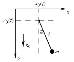
Figure 1: A pendulum with a moving suspension point placed in a variable gravitational field.

The Lagrangian of the system can be written as

$$L=\frac{m}{2}(\dot{x}^{2}+\dot{y}^{2})+mg_{x}x+m(g_{0}+g_{y})y$$ (2)

Using expressions (1) and ignoring non-dynamical terms and total derivatives, one transforms the Lagrangian to the final form:

$$L=\frac{1}{2}ml^{2}\dot{\alpha}^{2}-ml(\ddot{x}_{0}\sin\alpha+\ddot{y}_{0}\cos\alpha)+mg_{x}l\sin\alpha+m(g_{0}+g_{y})l\cos\alpha.$$ (3)

Now one can write down the equation of motion of the pendulum:

$$l\ddot{\alpha}=-\ddot{x}_{0}\cos\alpha+\ddot{y}_{0}\sin\alpha+g_{x}\cos\alpha-(g_{0}+g_{y})\sin\alpha.$$ (4)

We assume that the time-dependent components of the gravity vector are very small, $g_{x}(t)\ll g_{0}$, $g_{y}(t)\ll g_{0}$, and the acceleration of the suspension point $\ddot{y}_{0}$ is much smaller than the unperturbed gravity acceleration $g_{0}$. We also assume that $\alpha\ll 1$, $\sin\alpha\simeq\alpha$, $\cos\alpha\simeq 1$. Then, Eq. (4) simplifies:

$$\ddot{\alpha}+\omega_{p}^{2}\alpha=-\frac{\ddot{x}_{0}}{l}+\omega_{p}^{2}\alpha_{0}~{},$$ (5)

where $\omega^{2}_{p}=g_{0}/l$ is the square of oscillation frequency of the unperturbed pendulum. The angular variation of the local gravity vector $\bi{g}$, that is, the angular deviation of the local plumb line, is denoted $\alpha_{0}(t)=g_{x}(t)/g_{0}$. We see that, in the linear approximation in terms of $\alpha$, the pendulum behaviour is affected only by changes in the gravity force direction, namely, by the component $g_{x}$ of the gravity acceleration. The variations of the absolute value $|\bi{g}|$ and the component $g_{y}$ of the acceleration produce smaller effects, which we neglect.

Equation (5) is an inhomogeneous linear differential equation with constant coefficients. In the frequency domain, the relevant solution can be written

$$\alpha_{\omega}=\frac{\omega^{2}\,x_{0\omega}+l\omega_{p}^{2}\alpha_{0\omega}}{l\,(\omega_{p}^{2}-\omega^{2})},$$ (6)

where $\alpha_{\omega},\,x_{0\omega},\,\alpha_{0\omega}$ are complex Fourier amplitudes of the corresponding variables at frequency $\omega$. The divergent amplitude at the resonance frequency $\omega=\omega_{p}$ will be tempered by friction, which we have ignored. The regions of our interest are relatively high frequencies $\omega\gg\omega_{p}$ for astrophysical applications and relatively low frequencies $\omega\ll\omega_{p}$ for geophysical applications. For orientation, one can think of $\omega_{p}/2\pi=f_{p}\approx(0.1-1)~{}Hz$. This is true for the existing instruments.

a) High frequencies $\omega\gg\omega_{p}$ – astrophysical applications.
The pendulum angular amplitude is given by

$$\alpha_{\omega}\simeq\left[\left(\frac{\omega_{p}}{\omega}\right)^{2}-1\right]^{-1}\frac{x_{0\omega}}{l}-\left(\frac{\omega_{p}}{\omega}\right)^{2}\alpha_{0\omega}\simeq-\frac{x_{0\omega}}{l}-\left(\frac{\omega_{p}}{\omega}\right)^{2}\alpha_{0\omega}~{}.$$ (7)

The horizontal position of the pendulum mass is given by

$$x_{\omega} \simeq x_{0\omega}+l\alpha_{\omega}\simeq x_{0\omega}\left[1+\frac{1}{(\omega_{p}/\omega)^{2}-1}\right]-l\alpha_{0\omega}(\omega_{p}/\omega)^{2}$$ (8)

$$\simeq -\left(\frac{\omega_{p}}{\omega}\right)^{2}(x_{0\omega}+l\alpha_{0\omega})=-\left(\frac{\omega_{p}}{\omega}\right)^{2}x_{0\omega}-\frac{g_{x\omega}}{\omega^{2}}.$$

Eq.(8) illustrates the well known method of vibrational isolation of interferometer’s test masses-mirrors. The residual displacement $x_{\omega}$ of the pendulum mass is a factor $(\omega_{p}/\omega)^{2}$ smaller than the displacement $x_{0\omega}$ of the suspension point. The $N$ stages of isolation reduce the external $x_{0\omega}$ by a factor $(\omega_{p}/\omega)^{2N}$. This makes the mirror shielded from large deformational shifts of the suspension point, and therefore the interferometer becomes capable of detecting increadibly small distance variations caused by astrophysical signals. However, the displacement caused by the local gravitational environment (the last term in Eq.(8)), cannot be shielded. If this gravitational noise is present, it creates certain problems for the astrophysical program, which we will return to later.

b) Low frequencies $\omega\ll\omega_{p}$ – geophysical applications .
The pendulum angular amplitude is given by

$$\alpha_{\omega}\simeq\left(\frac{\omega}{\omega_{p}}\right)^{2}\frac{x_{0\omega}}{l}+\alpha_{0\omega}.$$ (9)

The contribution to $\alpha_{\omega}$ provided by movements of the suspension point (first term in Eq.(9)) is suppressed by a factor $(\omega/\omega_{p})^{2}$. At sufficiently low frequencies, this term can become smaller than the second term in Eq.(9). One can say that, in this regime, the equilibrium position of the pendulum follows a new plumb line $\alpha_{0\omega}$ determined by the slow variation $g_{x}(t)$ of the local gravity force vector $\bi{g}$.

The horizontal position of the pendulum mass, in the low-frequency approximation, is given by

$$x_{\omega}\simeq x_{0\omega}+l\alpha_{\omega}\simeq x_{0\omega}+\left(\frac{\omega}{\omega_{p}}\right)^{2}x_{0\omega}+l\alpha_{0\omega}\simeq x_{0\omega}+l\alpha_{0\omega}~{}.$$ (10)

It follows from Eq.(10) that the movements of the suspension point transmit practically without change into the movements of the pendulum mass. In other words, the low-frequency deformations cannot be shielded, so they should be monitored and compensated by the control systems.

The interferometer arm includes two separated pendula, and it is the difference of displacements and difference of mirrors’ inclinations that are actually being monitored. We assume that the pendula are identical, but their environments are different, see Fig.2.

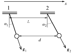
Figure 2: Relative variations of plumb lines and mass‘ positions in an interferometer.

We denote by symbol $\delta$ the variations at each site and by symbol $\Delta$ the difference of variations at two sites. It is important to know how different conditions are at two sites. If the characteristic spatial scale $\lambda$ of perturbations is shorter than $L$, then the conditions at two sites are not correlated, and $\Delta$-variations are typically of the same order of magnitude as the largest of individual $\delta$-variations. However, if both sites are covered by a long-wavelength perturbation $\lambda\gg L$, then the $\Delta$-variations are much smaller than the $\delta$-variations. Symbolically, we can write

$$\Delta\simeq\frac{L}{\lambda}\delta,~{}~{}~{}~{}~{}~{}~{}~{}{\rm if}~{}~{}~{}~{}~{}~{}~{}~{}L\ll\lambda.$$ (11)

Let the unperturbed coordinates of the suspension points be $x_{01},\,x_{02}$. Each point is subject to time-dependent deformational shifts $\delta{x_{01}},\,\delta{x_{02}}$. Of course, they are much smaller than the unperturbed distance $L$, $L=x_{02}-x_{01}$. We will also use the difference of the deformational shifts, $\Delta{x_{0}}(t)=\Delta L=\delta{x_{02}}(t)-\delta{x_{01}}(t)$. The difference of angular variables of the two pendula is $\Delta\alpha(t)=\alpha_{2}(t)-\alpha_{1}(t)$. The difference of local values of $g_{x}$ and, hence, the angle between the local plumb lines at two sites is $\Delta\alpha_{0}(t)=\alpha_{02}(t)-\alpha_{01}(t)$. [Here we ignore the fact that the Earth’s gravitational field is centrally-symmetric, which leads to slightly different orientations of the unperturbed gravity force vectors at two cites, but later we will take this fact into account.] Writing equations (5) at two sites, and taking their difference, we arrive at the equation

$$\ddot{\Delta\alpha}+\omega_{p}^{2}\Delta\alpha=-\frac{\ddot{\Delta x_{0}}}{l}+\omega_{p}^{2}\Delta\alpha_{0}~{}.$$ (12)

Certainly, the relevant solution to this equation is given by the formula similar to (6), with obvious substitutions:

$$\Delta\alpha_{\omega}=\frac{\omega^{2}\,\Delta x_{0\omega}+l\omega_{p}^{2}\Delta\alpha_{0\omega}}{l\,(\omega_{p}^{2}-\omega^{2})}.$$ (13)

The variation of distance between the masses is

$$\Delta d_{\omega}=\Delta{x_{0\omega}}+l\Delta\alpha_{\omega}.$$ (14)

The high-frequency and low-frequency approximations to equations (13), (14) follow the lines of equations (7), (8), (9), (10). In particular, in the low-frequency region, $\omega\ll\omega_{p}$, we have

$$\Delta\alpha_{\omega}\simeq\Delta\alpha_{0\omega}+\left(\frac{\omega}{\omega_{p}}\right)^{2}\frac{\Delta x_{0\omega}}{l}$$ (15)

and

$$\Delta d_{\omega}\simeq\Delta x_{0\omega}+l\Delta\alpha_{0\omega}~{}.$$ (16)

It is seen from Eq.(16) that the large deformational contribution $\Delta x_{0\omega}$ leaks into the system. This is why the interferometer’s adjustment system records and largely removes $\Delta x_{0\omega}$ from $\Delta d_{\omega}$ by applying force to the mirrors and mechanically adjusting their positions. (The adjustment system also tunes the frequency of the laser light). The circuits of adjustment system is one of the sources of geophysical information.

The angle $\Delta\alpha_{\omega}$ between the suspension wires, Eq.(15), is mostly the reflection of the angle between local plumb lines, first term in Eq.(15). For sufficiently low frequencies, the second term in Eq.(15) is smaller than the first one. We assume that the angle between the wires is at the same time the angle between surfaces of the mirrors. Under the condition that other contributions to Eq.(15) can be identified and separated (one complication, related to the centrally-symmetric character of the Earth’s gravitational field, is treated in detail in Sec.4c), the alighnment system, whose purpose is to monitor the angle between the mirrors, will be monitoring the angle $\Delta\alpha_{0\omega}$ between the plumb lines. This control system is another source of geophysical information.

Variables of geophysical interest, $\Delta x_{0\omega}$ and $\Delta\alpha_{0\omega}$, consist of two parts. One part is a useful geophysical signal, another part is environmental noise. In general, temporarily ignoring noises and other complications, the knowledge of the output signals $\Delta\alpha_{\omega}$ and $\Delta d_{\omega}$ allows one to solve equations (15), (16) with respect to $\Delta x_{0\omega}$ and $\Delta\alpha_{0\omega}$:

$$\Delta x_{0\omega}\simeq\Delta d_{\omega}-l\Delta\alpha_{\omega}~{},~{}~{}~{}~{}~{}~{}\Delta\alpha_{0\omega}\simeq\Delta\alpha_{\omega}-\left(\frac{\omega}{\omega_{p}}\right)^{2}\frac{\Delta d_{\omega}}{l}~{}.$$ (17)

Ideally, this would be a reconstruction, as complete as possible, of the acting geophysical perturbation. However, complications do exist, and we will perform more detailed analysis in the rest of the paper.

In the end of this section we shall briefly discuss the distance variations and plumb line deflections in terms of the Newtonian gravitational potential $U({\bf x},t)$ of the Earth. The potential $U$ is the sum of the unperturbed potential $U_{0}=GM/r$ and perturbations caused by external and internal gravitational fields. The external fields are mostly the tidal effects of the Moon, Sun and planets. The internal fields include such effects as normal oscillation modes of Earth and oscillations of the inner core of Earth. At the surface of an idealized rigid body, the local gravitational acceleration would be given by ${\bf g}=\partial U/\partial{\bf x}$. The true value of ${\bf g}$ at the surface of real elastic Earth is somewhat different from this quantity. This happens because the gravitational field perturbations, originating from either external or internal sources, displace elements of the Earth’s surface in its own gravitational field and also give rise to a redistribution of the Earth’s matter density. In the point of observations, these changes create additional variations of the gravitational potential. In conventional geophysics these effects are taken into account by some numerical factors called the Love numbers [10]. For a perfectly rigid body the Love numbers are zeros, while for a fluid body they are ones. On real deformable Earth, the Love numbers are roughly of the order of 1.

The difference of variations of ${\bf g}$ at two sites separated by $L$ is causing a change of distance between the sites, and it also determines a relative deflection of local plumb lines. Let the common unperturbed ${\bf g}_{0}$ point out in the $y$ direction, and the sites be located on the $x$ axis. Then, if $L$ is small in comparison with the characteristic length $\lambda$ at which the perturbation of the gravitational potential changes, one can derive:

$$\Delta\alpha_{0}=\frac{L}{g_{0}}\sqrt{\left(\frac{\partial g_{x}}{\partial x}\right)^{2}+\left(\frac{\partial g_{z}}{\partial x}\right)^{2}}=\frac{L}{g_{0}}\sqrt{\left(\frac{\partial^{2}U}{\partial x^{2}}\right)^{2}+\left(\frac{\partial^{2}U}{\partial z\partial x}\right)^{2}}.$$ (18)

It is clear that we are dealing with gradients of gravity variations $\delta{\bf g}$. A projection of this formula on the $x,y$ plane returns us to the results discussed above (compare with Eq.(11)):

$$\Delta\alpha_{0}=\frac{L}{g_{0}}\frac{\partial g_{x}}{\partial x}\approx\frac{\delta g}{g}\frac{L}{\lambda}\approx\delta\alpha\frac{L}{\lambda}.$$ (19)

3 Geophysical phenomena to be studied

A number of interesting geophysical phenomena are in fact geophysical signals that can be studied with the help of laser-beam detectors of gravitational waves. The division of geophysical phenomena into signals and noises is not clear-cut. For example, the low-frequency seismic perturbations can be assigned to either category. Likewise, periodic thermal deformations of land are probably the largest ones numerically, but they are not of gravitational origin, and we treat them as a predictable and removable hindrance rather than an interesting geophysical signal. In general, we shall regard signals some quasi-periodic processes with strong participation of gravity in them, whereas more random processes we regard noises, hampering detection of the signals. Noises are considered in the next section, while here we focus on some quasi-periodic phenomena which are believed to be important for global geodynamics. They are accompanied by variations of local gravity vector and land deformations. Both of these perturbations influence the performance of laser interferometric detectors of gravitational waves, and should be monitored and removed by the control systems.

a). The Earth tides.

Large perturbations of gravity ${\bf g}$ and deformations of land ${\bf u}$ are induced by the gravitational fields of the Moon and, to a smaller extent, Sun. The main tidal harmonics are well described and measured [10]. The values and directions of the perturbed quantities depend on the position of the observation point on the Earth surface, but we will be mostly interested in their typical (not exceptionally small and not exceptionally large) numerical amplitudes. The dominant contributor to the tidal effects is the lunar $M_{2}$ harmonic which has a period of $\tau\simeq 12~{}hours$ and which is quadrupolar in terms of its angular dependence. The typical $M_{2}$ amplitude of the variations of the absolute value of ${\bf g}$ is $\delta g\simeq 45~{}\mu Gal$ ($Gal=cm/sec^{2},~{}\mu Gal=10^{-6}~{}Gal,~{}nGal=10^{-9}~{}Gal$). The unperturbed gravity field is $g\simeq 980~{}Gal$, so that for the $M_{2}$ harmonic we have $\delta g/g\simeq 5\times 10^{-8}$. The main solar harmonic is $S_{2}$ with $\tau=12~{}hours$ and $\delta g\simeq 20~{}\mu Gal$. The higher frequency tidal harmonics are considerably weaker. For example: $M_{3}$ with $\tau\simeq 8~{}hours$, $\delta g\simeq 0.8~{}\mu Gal$ and $M_{4}$ with $\tau\simeq 6~{}hours$, $\delta g=0.03~{}\mu Gal$.

On the Earth surface, variations of gravity ${\bf g}$ and displacements ${\bf u}$ of land elements are linked by the Love numbers. If $W_{2}$ is the quadrupole component of the tidal potential, one can write for the radial components $\delta g_{r}$ and $u_{r}$ [10]:

$$\delta g_{r}=2(1+h-\frac{3}{2}k)\frac{W_{2}}{R_{e}},$$ (20)

$$u_{r}=\frac{h}{g}W_{2},$$ (21)

where $R_{e}$ is the Earth radius ($R_{e}\approx 6400~{}km$) and $h,k$ are the Love numbers ($h\approx 0.6,~{}k\approx 0.3$). Since the radial and angular components of the displacement vector ${\bf u}$ are approximately equal, we will be using for all of them the approximate relationship

$$u\approx 0.3~{}\frac{\delta g}{g}R_{e}.$$ (22)

This relationship is valid for any gravitational perturbation, not necessarily a tidal one. Specifically for the $M_{2}$ tidal component, a typical displacement amounts to $u\approx 10~{}cm$. The observed maximal displacements are a factor $3-5$ larger than this evaluation.

The characteristic spatial scale of the considered quadrupole perturbation is $\lambda\simeq R_{e}$. Therefore, assuming that the armlength of the interferometer is $L=3~{}km$, the $\Delta$-variation is smaller than the $\delta$-variation (see Eq.(11)) in proportion to $L/\lambda$, which reduces to

$$\frac{L}{R_{e}}\approx 5\times 10^{-4}.$$ (23)

Combining the numbers, we arrive at

$$\Delta x_{0} = u\frac{L}{R_{e}}=0.3~{}\frac{\delta g}{g}L\approx 5\times 10^{-3}~{}cm,~{}~{}~{}~{}~{}~{}{\rm and}$$

$$\Delta\alpha_{0} = \frac{\delta g}{g}\frac{L}{R_{e}}\approx 3\times 10^{-11}~{}{\rm rad}.$$ (24)

As was already mentioned, tidal perturbations of this level of magnitude should be easily seen by the interferometer control systems. A successful performance of the interferometer requires a much better precision in monitoring the distance between mirrors, at the level not less than $(10^{-6}-10^{-7})~{}cm$. The danger of tidal effects for the LIGO interferometers and the necessity of their removal have been long recognised [11]. We focus on the positive side of this necessary procedure: the existing network of interferometers, located in different parts of the globe, will allow one to obtain useful information on amplitudes, spatial patterns and temporal phases of tidal perturbations. This collected and analyzed low-frequency information will help refine numerical values of Earth’s parameters, such, for example, as its Love numbers.

b). Free oscillations of Earth.

As every elastic body, our planet is capable of free oscillations (see, for example, [12]). In the approximation of a non-rotating, uniform, spherically-symmetric Earth, it is convenient to expand perturbations in terms of spherical harmonics $Y_{lm}(\theta,\phi)$, where $\phi$ is longitude and $\theta$ is co-latitude:

$$u(r,\theta,\phi)\sim~{}~{}{{}_{n}R_{l}(kr)}\,Y_{lm}(\theta,\phi)\,\exp\left(i\omega t\right).$$ (25)

The discrete values of the wave number $k$, $k_{ln}=\pi\alpha_{ln}/R_{e}$, are determined by the radial boundary conditions and the $n$-th root, $\alpha_{ln}$, of the corresponding boundary equation (see, for example, [13]). The eigen-frequencies $\omega$ do not depend on $m$ and are given by $\omega_{ln}=\pi\alpha_{ln}c_{s}/R_{e}$, where $c_{s}$ is the appropriate speed of sound. If the multipole order $l$ is much smaller than a (nonzero) $n$, the deformations have maximal amplitudes in the central region of the sphere. In the opposite case of $l$ being much larger than $n$, the deformations are mostly concentrated near the surface of the sphere, and it also holds that $\pi\alpha_{ln}\approx l$. In the extreme regime $l\gg n$, the deformations look more like seismic perturbations rather than free oscillations of Earth. The short-wavelength seismic perturbations can propagate deep to the central regions of Earth, refract and reflect back. This is an important diagnostic of the central regions.

There are two basic types of elastic deformations. One is accompanied by variations of volume, matter density and gravity ${\bf g}$, and is called spheroidal modes ${}_{n}S_{lm}$. Another is not accompanied by these variations; it represents purely twisting motions, and is called toroidal (shear) modes ${}_{n}T_{lm}$. Some of the shear perturbations cannot propagate in liquids, and their observed attenuation in the central regions of Earth helped discover the liquid (outer) core. Many hundreds of Earth’s normal modes are now identified from the study of ground motions and gravimeter records. The longest period normal mode is ${}_{0}S_{2}$ with period $T=53.8~{}min$. This period is of course consistent with our evaluations given above. Taking $c_{s}\approx 4~{}km/sec$ and $\alpha_{20}\approx 1$, we arrive at the right value for $T$. The frequency of the ${}_{0}S_{2}$ mode is $f\approx 3\times 10^{-4}~{}Hz$, whereas the frequencies of higher order $S$ and $T$ modes extend to the $milli~{}Hz$ region. For example, the ${}_{0}S_{20}-{{}_{0}S_{40}}$ modes ($l=20-40$) have equally spaced frequencies in the interval of approximately $(1-5)~{}mHz$, again in agreement with the evaluations given above.

Free oscillations of Earth are best observed after large earthquakes. In contrast to tidal harmonics, the amplitudes of free Earth oscillations cannot be predicted in advance. However, it is known that typical observed values of gravity variations in the fundamental ${}_{0}S_{2}$ mode are at the level of about 1 $\mu Gal$ [14, 15, 16]. The amplitudes of higher frequency registered modes are smaller, but they can reach $\delta g\sim 0.1$ $\mu Gal$. The amplitudes of modestly excited modes between ${}_{0}S_{20}$ and ${}_{0}S_{40}$ were detected in the long series of observations on seismically quiet days. The acceleration amplitudes are at the level of $2~{}nGal$, and higher [17]. There exists the permanently present noise in these modes with the amplitudes corresponding to $0.4~{}nGal$. Interestingly, this background level of land deformations and gravity variations cannot be explained by cumulative effect of small earthquakes, despite the fact that there occur thousands of them per year. It is suggested [17] to seek the source of these continuous oscillations of Earth in the action of atmospheric pressure variations on the Earth surface. We will return to this discussion in our analysis of atmospheric noises in Sec.4b.

The modestly excited higher frequency $S$ and $T$ modes seem to be within the reach of adjustment and alighnment systems of the gravity-wave detectors. The $T$ modes do not affect the plumb line directions, but they are present in the distance variations. Let us take a representative normal mode with $f=4\times 10^{-3}~{}Hz$ and the amplitude of gravity variations $\delta g=2~{}nGal$, i.e. $\delta g/g=2\times 10^{-12}$. The wavelength $\lambda$ is $\lambda=c_{s}/f\approx 10^{8}~{}cm$, that is, the spatial scale of perturbations $\lambda$ is smaller than $R_{e}$, but still much longer than the armlength $L=3~{}km$ of the interferometer.

We shall first generalise Eqs. (22), (3) to the case, where the spatial scale of $\delta g$ is $\lambda$, not $R_{e}$. Then, we will have to write

$$\Delta x_{0}\approx 0.3~{}\frac{\delta g}{g}R_{e}\frac{L}{\lambda}~{}~{}~{}~{}~{}~{}{\rm and}~{}~{}~{}~{}~{}~{}\Delta\alpha_{0}\approx\frac{\delta g}{g}\frac{L}{\lambda}.$$ (26)

Note that, on the surface of deformable Earth, there exists a universal relationship between the distance and angle variations, which directly follows from Eq.(26):

$$\Delta\alpha_{0}\approx\frac{\Delta x_{0}}{0.3~{}R_{e}}.$$ (27)

Substituting the numbers in Eq.(26), we obtain the following evaluations for the considered normal mode of oscillations at $f=4\times 10^{-3}~{}Hz$:

$$\Delta x_{0}\approx 10^{-6}~{}cm,~{}~{}~{}~{}~{}{\rm and}~{}~{}~{}~{}~{}~{}\Delta\alpha_{0}\approx 6\times 10^{-15}~{}rad.$$ (28)

Obviously, if the amplitude of the excited mode is larger than $2~{}nGal$, this will increase the expected amplitudes of $\Delta x_{0}$ and $\Delta\alpha_{0}$. In addition, normal modes, as any other oscillations, are characterised by certain quality factor $Q$. The mode can execute $Q$ cycles before its amplitude degrades by a factor of 3, or so. If the observation of the mode lasts for at least as long as its relaxation time $\tau$, $\tau=Q/\omega$, the signal to noise ratio increases in proportion to $\sqrt{Q}$. This makes the prospects of detection of the Earth normal modes much better. The quality factor of individual modes is uncertain, but the literature often quotes the numbers well in excess of 100 (see, for example, [18]).

c). The Earth inner core oscillations

The oscillations of the real Earth are complicated by Earth’s aspherical shape, its rotation, the presence of gravitational restoring forces in addition to elastic forces, the stratification and variation of material properties with depth, etc. Very important modifications are caused by the existence of the Earth core (see, for example, [18]). It is believed that the inner core is solid and has radius $r_{s}\approx 1220~{}km$ and density $\rho_{s}\approx 13~{}g/cm^{3}$. The outer core is liquid and has radius $r_{l}\approx 3470~{}km$ and density $\rho_{l}\approx 12.6~{}g/cm^{3}$. [The current geophysical models claim a much higher precision of the Earth parameters than is actually needed for our evaluations.]

The solid core is held in its equilibrium position within the liquid core mainly by gravitational forces. It is reasonable to expect that an earthquake, or some other cause, can occasionally excite oscillations of the inner core, predominantly along the Earth rotation axis (the polar mode) [16, 19]. A displacement of a solid sphere within a liquid sphere is equivalent to a displacement of the effective mass $m=(4\pi/3)(\rho_{s}-\rho_{l})r_{s}^{~{}3}$. If the amplitude of the displacement is $A$, then the associated variation of gravity at the Earth surface is

$$\delta g=\frac{2Gm}{R_{e}^{3}}A=\frac{8\pi}{3}GA(\rho_{s}-\rho_{l})\left(\frac{r_{s}}{R_{e}}\right)^{3}.$$

The evaluation of this expression using the parameters mentioned above gives

$$\delta g\approx 2~{}nGal~{}\left(\frac{A}{cm}\right).$$

Period $T_{p}$ of polar oscillations of the inner core mass $m_{s}$ is mainly determined by the gravitational restoring force:

$$m_{s}{\ddot{A}}=-G\frac{m~{}\frac{4}{3}\pi\rho_{l}A^{3}}{A^{2}},$$

which leads to $T_{p}^{2}=3\pi\rho_{s}/G\rho_{l}(\rho_{s}-\rho_{l})$. Corrections to this expression are taken into account by a small numerical factor $\alpha_{p}$ [19], so that

$$T_{p}\simeq\sqrt{\frac{3\pi(\rho_{s}+\alpha_{p}\rho_{l})}{G\rho_{l}(\rho_{s}-\rho_{l})}}.$$ (29)

The evaluation of $T_{p}$ leads to a period of about 4 hours. The Coriolis force of the rotating Earth splits this period inito a triplet of periods, with the size of splitting determined by the Earth angular velocity.

The fascinating phenomenon of the inner core oscillations will be in the center of our further discussion. There exist indications that the inner core translational triplet has been actually detected [20, 21]. The analysis of long records from superconducting gravimeters has shown three resonances with the central period $T_{C}\approx 3.8~{}hours$ and the side periods separated from the central one by $\sim\pm 10~{}min$. The amplitudes of each of the three oscillations are at the level of $(5-6)~{}nGal$. The quality factor $Q$ of each resonance is somewhat higher than 100.

Using evaluations similar to those that have been done in previous subsections, we can estimate the effect of the Earth inner core oscillations on the laser-beam detectors of gravitational waves. We take the amplitude of gravity variations $\delta g/g=6\times 10^{-12}$, the charecteristic spatial scale of gravity variations and land deformations $\lambda_{c}\simeq 2~{}R_{e}$, and the length of the interferometer arm $L=3~{}km$. Then, the distance and angular signal amplitudes amount to

$$\Delta x_{0}\approx 3\times 10^{-7}~{}cm,~{}~{}~{}~{}~{}{\rm and}~{}~{}~{}~{}~{}~{}\Delta\alpha_{0}\approx 2\times 10^{-15}~{}rad.$$ (30)

The detectability condition requires that the signal to noise ratio $S/N$ should be better than 1. The resonance bandwidth of the core oscillations is $\Delta f=f_{C}/Q$, where the central resonance frequency is $f_{C}=7.3\times 10^{-5}~{}Hz$. We assume that the observation time of the signal is at least as long as $Q$ cycles of the signal. This means that the tolerable spectral noise ${\tilde{N}}$ per $\sqrt{Hz}$ is related to the signal amplitude $S$ according to

$${\tilde{N}}~{}\sqrt{\Delta f}=N<S.$$ (31)

Although the quality factor $Q$ for the Earth inner core oscilllations is somewhat larger than 100, we take it as $Q=73$ in order to operate with the round number: $\sqrt{f_{C}/Q}=10^{-3}$.

Thus, we derive the allowed broadband noises in the region of resonances:

$${\Delta x}_{noise}\approx 3\times 10^{-4}~{}\frac{cm}{\sqrt{Hz}}, ~{}~{}~{}~{}~{}~{}{\Delta\alpha}_{noise}\approx 2\times 10^{-12}~{}\frac{rad}{\sqrt{Hz}},$$ (32)

$${\delta g}_{noise}\approx 6~{}\frac{\mu Gal}{\sqrt{Hz}}.$$

The relationship between the noise variables in Eq.(32) is of course the same as the relationship between the signal variables, Eq.(26) with $\lambda\simeq R_{e}$.

Obviously, if for some reason the inner core gets excited to the level much higher than $5-6~{}nGal$, the requirements on the tolerable noise could be significantly relaxed. Alternatively, if the noise remains at the level of Eq.(32), the $S/N$ gets much higher than 1. For example, there exists evidence [16] that the amplitude of the inner core oscillations can be as large as $0.64~{}\mu Gal$, which would make the signal easily detectable. And, in any case, one can further improve $S/N$ by observing for longer time than the assumed 73 cycles.

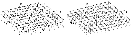
Figure 3: Gravity vectors describing tides and oscillations of the Earth inner core. Two distributions shown on the panels are separated by a half of the tidal period.

Variations of gravity on the Earth surface within a patch of the size $L=3~{}km$ can be numerically simulated [22]. Fig.3 is the illustration of the gravity field vectors disturbed by the inner core polar motion and by semidiurnal tides. To make the core contribution distinguishable on the graph, it was artificially enhanced by a factor 1000.

4 Environmental and instrumental noises

The important geophysical phenomena listed in the previous section will certainly affect the laser-beam detectors of gravitational waves. However, they can only be measured if the signals are not swamped by various noises. In principle, any random fluctuations of the Earth surface and any random redistributions of the surrounding masses of soil, air and water can alter the distances and plumb line directions, which we are interested in. In addition to these environmental noises, there always exist imperfections in the measuring devices themselves, that is, instrumental noises. Here, we will analyse the noises which we consider most dangerous for the proposed measurements.

a) Seismic perturbations

It has been long recognized that seismic waves propagating in the vicinity of a laser interferometer can limit its performance as a gravitational wave detector [25, 26, 27]. The usual region of concern are frequencies around $10~{}Hz$, where the expected noise can be dangerous for the planned advanced g.w. interferometers. In contrast, we are concerned with perturbations at much lower frequencies, $\sim 10^{-4}~{}Hz$, and with their effect on the control systems of the already operating initial interferometers. Some families of seismic perturbations are not accompanied by variations of matter density and, hence, they are not accompanied by variations of local gravity. This sort of perturbations cannot directly affect the plumb lines. However, all seismic perturbations can change the distance between the points on the Earth surface.

We will extrapolate the often used spectra of the seismic (displacement) noise to the frequencies of geophysical interest. For a discussion of seismic noises, including those that were measured at the interferometer cites, see, for example, [25, 26, 27, 28, 29, 30, 31]. The displacement noise is normally presented in terms of spectral density $u_{f}$ written in units of $cm/\sqrt{Hz}$: $u_{f}=Af^{-\gamma}$. The mean-square value of the random quantity $u$ within a bandwidth from $f_{min}$ to $f_{max}$ is defined by

$$\langle u^{2}\rangle=\int_{f_{min}}^{f_{max}}(u_{f})^{2}df.$$ (33)

The spectral index $\gamma$ vary from one spectral interval to another, but there exist indications that $\gamma\simeq 1$ at frequencies below $0.1~{}Hz$, so we will adopt $\gamma=1$. The coefficient $A$ is also uncertain. It varies from site to site, and there exist a broad range of estimates. We will adopt some averaged value $A=10^{-4}~{}cm/\sqrt{Hz}$ at $f<0.1~{}Hz$. So, we shall be working with the spectrum

$$u_{f}=10^{-4}\left(\frac{10^{-1}Hz}{f}\right)~{}\frac{cm}{\sqrt{Hz}}.$$ (34)

Surely, at very low frequencies, the concept of seismic perturbations overlaps with the concept of the Earth free oscillations, so the estimates should be consistent with each other and with the gravimeter records.

To find the differential noise spectral density $\Delta x_{seism}$, we have to multiply Eq.(34) with $L/\lambda=Lf/c_{s}$. Assuming that $c_{s}$ does not significantly depend on $f$, the frequency dependence cancels out in the product, and the amount of seismic noise is expected to be approximately equal at all geophysical frequencies. We want to use one simple formula in the broad interval of frequencies, so we put $c_{s}=1~{}km/sec$ for this calculation. Then, using $L=3~{}km$, we arrive at

$$\Delta x_{seism}\approx 3\times 10^{-5}~{}\frac{cm}{\sqrt{Hz}}.$$ (35)

This estimate is a factor of 10 lower than the level of tolerable noise in Eq.(32). It shows that this source of noise cannot prevent the observation of the Earth inner core oscillations by the adjustment system of laser interferometers.

To check the consistency of our evaluations, it is instructive to estimate the upper bound of gravity variations caused by seismic perturbations. This evaluation of seismic $\delta g_{f}$ will also be helpful in the next subsection where we are considering atmospheric fluctuations. We will have to compare our estimations with the actually measured (total) values of the acceleration noise $\delta g_{f}$ at the core oscillation frequencies around $f_{C}$ and normal mode $mHz$ frequencies (compare, for example, with [32, 21, 20, 17]):

$$\delta g_{f}\approx 0.5~{}\left(\frac{10^{-4}~{}Hz}{f}\right)~{}\frac{\mu Gal}{\sqrt{Hz}}.$$ (36)

A matter density wave, with the amplitude of density variations $\delta\rho/\rho$ and wavelength $\lambda$, produces a local variation of gravity with the amplitude $\delta g/g(\lambda)\sim\delta\rho/\rho\sim u/\lambda$, where $g(\lambda)/g\approx\lambda/R_{e}$. We take into account the finite rigidity of Earth, expressed by the Love numbers, and write $0.3~{}\delta g/g(\lambda)\approx u/\lambda$, that is,

$$0.3~{}\frac{\delta g}{g}\approx\frac{u}{R_{e}}.$$ (37)

Surely, this formula is consistent with Eq.(22). Using Eq.(34) in this formula, we arrive at the estimate for seismic $\delta g_{f}$, which turns out to be at the level of the observed variations, Eq.(36).

The estimate (36) can now be translated into the spectral noise contribution to $\Delta\alpha_{0}$ caused by seismic perturbations. It is seen from Eq.(26) that the $f$-dependence cancels out, so we derive

$$\Delta\alpha_{seism}\approx 10^{-13}~{}\frac{rad}{\sqrt{Hz}}.$$ (38)

This noise is lower that the tolerable level of noise in Eq.(32). Therefore, the alighnment system of laser interferometers can also be used, barring some complications discussed below, for observation of the inner core oscillations.

b) Atmospheric noises

It is somewhat surprising that the movement of light air in the Earth atmosphere can be a more serious source of noise for the proposed measurements than the movement of heavy soil in seismic perturbations. We will illustrate this statement with a simple theory of gravity variations and land deformations caused by atmospheric motions.

Consider an air density inhomegeneity with the amplitude $\delta\rho/\rho$ and a characteristic spatial scale $\lambda$. Let this scale be shorter than the characteristic height of the Earth atmosphere $H$. In a point of observation at the Earth surface, the variation of $g$ is mostly determined by the variation of mass $\delta m$ in a volume $\lambda^{3}$ with the center located at a distance $\lambda$ from the observer. More distant volumes give smaller contributions to $\delta g$ and can be ignored. So, we could write:

$$\delta g\approx\frac{G~{}\delta m}{\lambda^{2}}\approx G~{}\delta\rho~{}\lambda.$$

This expression is adequate for $\lambda<H$. However, we are mostly interested in the opposite case $\lambda>H$. As will be clear from discussion below, it is time-dependent atmospheric variations at these longer scales that fall in the frequency range of geophysical interest. Therefore, we have to consider variations of mass in a volume $H\lambda^{2}$, rather than $\lambda^{3}$. The center of this flattened volume is located at a distance $\lambda$ from the observer. The expression for $\delta g$, appropriate for scales and frequencies of our interest, should be written as

$$\delta g\approx\frac{G~{}\delta m}{\lambda^{2}}\approx G~{}\delta\rho~{}H.$$ (39)

Variations of air density $\delta\rho$ are more difficult to measure than variations of pressure, so one usually operates with the (spectral) pressure variations $\delta p_{f}=c_{a}^{~{}2}~{}\delta\rho_{f}$, where the square of the air sound speed is $c_{a}^{~{}2}\simeq 10^{9}~{}cm^{2}/sec^{2}$. Then, equation (39) takes the form

$$\delta g_{f}\approx G~{}\frac{\delta p_{f}}{c_{a}^{~{}2}}~{}H.$$ (40)

The question arises which $\delta p_{f}$ should be used in this equation in order to estimate $\delta g_{f}$.

The observations indicate [33, 34, 35, 36, 37, 17] that, during relatively quiet times, the spectral pressure variations behave, roughly, as $\delta p_{f}\propto f^{-1}$. This frequency dependence is close to the Kolmgorov-Obukhov law for atmospheric turbulence [38, 37] $\delta p_{f}\propto f^{-7/6}$. In the frequency interval $\sim(10^{-5}-10^{-2})~{}Hz$, observational data can be approximately fitted by the formula

$$\delta p_{f}=200\left(\frac{f}{10^{-4}Hz}\right)^{-1}~{}\frac{Pa}{\sqrt{Hz}},$$ (41)

where the unit of pressure $Pa$ is $Pa=10~{}g/cm~{}sec^{2}$. The replacement of the spectral index $(-1)$ by the genuine Kolmogorov-Obukhov index $(-7/6)$ leaves the fit equally good.

A purely turbulent $\delta p_{f}$ raises certain concerns, as it is not obvious that turbulence can directly contribute to $\delta g$. Turbulence describes chaotic velocities in a medium and variations of the medium’s kinetic pressure, but these variations are not necessarily accompanied by variations of the medium’s mass density $\delta\rho$ and gravity $\delta g$. [There exists, however, an indirect influence of air turbulence on $g$ through the land deformations excited by the variable pressure. We will discuss this issue separately, at the end of this subsection.] On the other hand, transportation and mixing of cold and hot air, caused by the turbulence, does contribute to $\delta\rho$ and, hence, directly contributes to $\delta g$. Without analysing the true nature of the observed $\delta p_{f}$, we will be using the observed spectrum (41) in the expression (40).

Combining Eq.(41) and Eq.(40), and using numerical values of the participating quantities, including the effective height of the atmosphere $H\approx 10~{}km$, we arrive at

$$\delta g_{f}\approx 0.2~{}\left(\frac{10^{-4}Hz}{f}\right)~{}\frac{\mu Gal}{\sqrt{Hz}}.$$ (42)

This evaluated $\delta g_{f}$ is smaller than, and is consistent with, the observed (total) variations $\delta g_{f}$ approximated by Eq.(36).

To evaluate the contribution of the atmospheric $\delta g_{f}$ to the noises in distance and angular measurements (see Eq.(26)), we first need to find out the characteristic correlation length $\lambda$, as a function of frequency $f$. To do this, we have used experimental data which were kindly provided to us by the Japanese Weather Association. These data were collected by the Meteorological National Geographical Institute at the set of meteo-stations near Tsukubo Scientific Center. The total area of $20\times 20~{}km$ is covered by $10$ stations. The average distance between nearby stations is $10~{}km$. The pressure data were recorded at each station with a sample time $1~{}min$. The length of the analysed record was $1~{}month$.

Using the experimental data, we have built temporal spectra of pressure $S_{p}(f)$ measured at each station, and also temporal spectra of difference of pressure $S_{\Delta p}(f)$ at each pair of neighbouring stations. Because of the spatial correlation of the data, the spectral components of the difference of pressure $S_{\Delta p}(f)$ prove to be smaller than the approximately equal spectral components of pressure $S_{p}(f)$ measured at each station. For each pair of stations, the spatial correlation scale $\lambda(f)$ was estimated from the relationship

$$\lambda(f)=r\frac{2S_{p}(f)}{S_{\Delta p}(f)}.$$

Then, the found quantities $\lambda(f)$ were avaraged over all pairs of stations. As a result, we have arrived at the mean value of $\lambda(f)$:

$$\lambda(f)=500~{}\left(\frac{10^{-4}Hz}{f}\right)~{}km.$$ (43)

It also follows from the data that this number depends on overall meteorological conditions and can change by a factor $2-3$.

The evaluations (43), (42) should now be used in general formulas (26). We arrive at the expected atmospheric noise contribution:

$${\Delta x}_{atm}\approx 2\times 10^{-4}~{}\frac{cm}{\sqrt{Hz}},~{}~{}~{}~{}~{}{\rm and}~{}~{}~{}~{}{\Delta\alpha}_{atm}\approx 10^{-12}~{}\frac{rad}{\sqrt{Hz}}.$$ (44)

These estimates are marginally consistent with the level of allowed noise defined by Eq.(32).

It is satisfying that the differential displacement noise (44) is consistent with the direct estimate of land deformations, supposedly excited by atmospheric turbulence [17]. The permanently present amplitudes of acceleration $a_{n}$ at $mHz$ frequencies of the Earth’s eigen-modes are all approximately at the level of $0.4~{}nGal$ [17]. Taking $3~{}mHz$ as the central frequency, the discrete set of these observed modal amplitudes $a_{n}$ can be translated into an interval of a continuous acceleration spectrum

$$a_{f}\approx 0.4~{}\frac{1}{\sqrt{3\times 10^{-3}}}~{}\frac{nGal}{\sqrt{Hz}}\approx 7~{}\frac{nGal}{\sqrt{Hz}}.$$ (45)

The observed accelerations $a_{f}$ are associated with the periodic displacements $u_{f}$ of the land elements:

$$u_{f}\approx\frac{a_{f}}{(2\pi)^{2}f^{2}}\approx 10^{-9}~{}\frac{1}{f^{2}}~{}\frac{cm}{\sqrt{Hz}}.$$ (46)

The corresponding spectral noise amplitude of the distance variation between the interferometer’s mirrors, separated by $L=3~{}km$, will amount to

$$\Delta x_{f}\approx u_{f}\frac{Lf}{c_{s}}\approx 3\times 10^{-9}~{}\frac{1}{f}~{}\frac{cm}{\sqrt{Hz}}.$$ (47)

We extrapolate this formula to lower frequencies, including the interval around $f_{C}$. Then, at $f=f_{C}$, we obtain

$$\Delta x_{f}\approx 5\times 10^{-5}~{}\frac{cm}{\sqrt{Hz}}.$$ (48)

This estimate is perfectly consistent with the independent evaluation that we have derived in Eq.(44).

To conclude this subsection, we can say that the expected atmospheric noise is marginally acceptable for the proposed geophysical measurements with laser-beam detectors of gravitational waves. It is likely that some rare events, such as passing cyclones and atmospheric fronts, can produce larger disturbances than the estimates (44), but these atmospheric events can be anticipated and excluded from the data.

c) Coupling of noises in distance and angle measurements

As was already discussed above, variations of the Earth’s gravitational field, caused either by external or internal sources, produce changes in, both, distance between the sites and angle between the plumb line directions on the Earth surface. It is only on the surface of an idealized perfectly rigid body that the change of angle between the plumb lines is not accompanied by distance variations. And it is only in an idealized homogeneous gravitational field, or during spherically-symmetric oscillations of a homogeneous sphere, that the change of distance between the sites is not accompanied by the change of angle between the plumb lines. While describing geophysical signals, we have already noticed this important link between $\Delta x_{0}$ and $\Delta\alpha_{0}$, see Eq.(27). For example, as we know, the Earth inner core oscillations can lead to distance variations with the amplitude $\Delta x_{0}=3\times 10^{-7}~{}cm$, and they will necessarily be accompanied by the angle variations with the amplitude $\Delta\alpha_{0}=2\times 10^{-15}~{}rad.$ However, even in the absence of any geophysical signal, a similar link exists between the random (noisy) parts of $\Delta x_{0}$ and $\Delta\alpha_{0}$.

Fig.4 illustrates the appearance of noise in the channel of angle measurements, if there exists noise in the channel of distance measurements. The fluctuating part $\Delta L$ of distance between the sites (independently of the reasons why this fluctuating part exists) translates into the fluctuating part $\alpha_{gn}$ of angle between the plumb lines, $\alpha_{gn}\sim\Delta L/R_{e}$. This coupling takes place simply because of the centrally-symmetric character of the Earth’s gravitational field. [We ignored this fact in derivation of Eq.(15), but otherwise a term proportional to $\Delta x_{0\omega}/R_{e}$ should have been added to the right-hand-side of that equation.] Therefore, signals and noises in the two channels are linked by essentially one and the same relationship:

$$\Delta\alpha\approx\frac{\Delta x}{R_{e}}.$$ (49)

This equation gives the minimal and unavoidable level of noise in angles, which arises because of the noise in distances. Other reasons (for example, related to local inhomogeneities on two sites) can only make this relationship more complicated. However, even the simplified link represented by Eq.(49) leads to an important conclusion: there is no special advantage in measuring angles through the alignment control system, rather than measuring distances through the adjustment control system; the signal-to-noise ratios are practically equal in these channels. On the other hand, the use of both channels, instead of only one of them, would certainly increase the reliability of geophysical detection. In particular, the combined information will help identify and remove the distance variations caused by quasi-periodic thermal deformations of the Earth surface. Moreover, if both the distance and angles between mirrors are accurately measured (including their noisy contributions), then the use of Eq.(49) for noises (or, preferably, the use of a more precise version of this equation) would allow one to subtract from the measured angle that part of the angle which arises purely due to the coupling. This procedure would help identify that part of the measured angle which is caused specifically by the variation of plumb lines.

It turns out, however, that the angle measurements by the actually existing alignment systems have their own difficulties and ambiguities. We will fully address them in Sec.5.

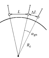
Figure 4: Coupling of signals and noises in distances and angles

d) Instrumental noises

It appears that instrumental noises will not be a major problem for the proposed geophysical studies. This is not surprising, as the gravitational-wave detectors implement the best currently available technology aimed at measuring much weaker gravitational signals. Obviously, geophysical signals have different origin and are concentrated in a substantially different frequency band, but in both cases we are dealing with manifestations of the same force - gravitation.

The tolerable noise of Eq.(32) implies that the accuracy of the adjustment system is better than $3\times 10^{-6}~{}cm$ at frequencies around $10^{-4}~{}Hz$. Adjustment systems of the presently operating interferometers satisfy this requirement, but, in order to ensure a successful performance of the interferometer as a g.w. detector, they may not need the low-frequency precision higher than $10^{-7}~{}cm$. Certainly, the advanced interferometers will require an enhanced precision of the adjustment systems in the ‘control band’ of frequencies. This is necessary in order to assure that only very small forces are applied to the mirrors themselves [39]. In any case, from the instrumental point of view, the accuracy of the adjustment system can be made much better than presently achieved. Even smaller variations, at the level of $10^{-13}cm$, can be detected by the interferometer adjustment system, if the dominant noise is reduced to the photon shot noise [40, 41]. The photon noise limited spectral sensitivity is basically determined by the relationship

$$\Delta x_{instr}\simeq\frac{\lambda}{F}\sqrt{\frac{\hbar\omega}{\eta P}},$$ (50)

where $\lambda$ is the wavelength of the laser light and $\omega=2\pi c/\lambda$ is its frequency, $F$ is the cavity finesse, $P$ is the optical power available at the photodector and $\eta$ is its efficiency. Taking reasonable parameters $\lambda=10^{-4}~{}cm$, $F=100$, $P=100~{}mW$, $\eta=0.9$ we arrive at

$$\Delta x_{instr}\approx 1.5\times 10^{-15}~{}~{}\frac{cm}{\sqrt{Hz}}.$$ (51)

This number can be improved by the increase of $P$. Therefore, we do not expect instrumental noises in the adjustment system to be a limiting factor for the measurement of geophysical signals described by Eqs. (28), (30). Obviously, we assume that the extra noises (above purely photon noise) are not excessively large.

The purpose of the alignment system is to monitor and remove possible misalignments between the laser beam and the axis of optical resonator formed by the corner mirror and the end mirror. One reason for this misalignment to arise is precisely the deviation of plumb lines caused by a geophysical signal and, hence, the change of angle between mirrors. In principle, the existing alignment systems are very sensitive to a possible change of angle between mirrors. If the dominant noise is the photon shot noise, the angular spectral precision of the alignment system can reach [42, 43, 22, 44]:

$$\Delta\alpha_{instr}\simeq\frac{\lambda}{w_{0}}\sqrt{\frac{\hbar\omega}{\eta P}},$$ (52)

where $w_{0}$ is the diameter of the laser beam ‘waist’. Taking the same parameters as before and $w_{0}=0.1~{}cm$, we arrive at

$$\Delta\alpha_{instr}\approx 1.5\times 10^{-12}~{}~{}\frac{rad}{\sqrt{Hz}}.$$ (53)

This accuracy is at the level of the tolerable noise of Eq.(32), but it can be improved by the increase of $P$. We cautiously conclude that the instrumental noise of alignment systems will not swamp the expected geophysical signal.

A more fundamental problem with the existing alignment systems lies, however, in a different place. The error signal of the system cannot tell us whether the misalignment arose because of the change of angle between the mirrors or because of the change of lateral position of the end spherical mirror. The first cause is what we are interested in, while the second cause could be simply an unrelated noise. Without solving this problem, one would not be able to use angular measurements as an additional source of geophysical information. This is why we address this problem in next sections.

5 Measurement of mirrors’ tilts

Here, we will consider in more detail the response of a g.w. interferometer to the deformations of Earth’s surface and variations of local gravity. To be specific, we will do this on the example of the VIRGO observatory [7].

Each arm of the VIRGO interferometer consists of an asymmetric Fabry-Perot optical resonator, which is formed by a flat front mirror and a spherical end mirror. The length of each arm is $L=3~{}km$. The laser beam enters the resonator through the partially transparent front mirror. Each mirror is hanging on a multi-stage support, which behaves as a single wire pendulum at frequencies below $1~{}Hz$. The source of light itself is located very close (at a distance less than $20~{}m$) to the front mirror, so one can neglect the gradients of local gravity and deformations of land at such short distances. Therefore, we shall accept, for simplicity, that in the chosen coordinate system the front flat mirror does not move, the laser beam is always orthogonal to the front mirror, and the beam enters the resonator from one and the same point on the flat mirror. The problem is still sufficiently general, as the main trouble arises when one considers the relative position and orientation of the remote spherical mirror with respect to the front mirror and laser beam.

The optical axis of the resonator is orthogonal to the flat mirror and goes through the center of curvature of the spherical mirror. The curvature radius $r$ of the spherical mirror is approximately equal to the distance between the mirrors, so we take $r=3~{}km$. In the tuned working condition, the laser beam is aligned with the optical axis. In this configuration, all light participates in interference, and the sensitivity is maximal. A misalignment between the beam and optical axis is sensed by the changing spatial distribution of the electromagnetic field in the Fabry-Perot cavity [42, 45]. Since we have assumed that the beam is always orthogonal to the flat mirror, the misalignment can only arise if the spherical mirror inclines with respect to the beam, or changes its position in the plane orthogonal to the beam. These possible motions of the end mirror, in the $(x,y)$-plane containing the beam, are shown in Fig.5.

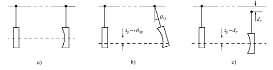
Figure 5: Misalignment of the optical axis in the Fabry-Perot interferometer: a) aligned configuration, b) tilt of the spherical mirror, c) vertical shift of the spherical mirror

A technical advantage of this alignment control system (which turns out to be a big disadvantage for geophysical applications) is in that the system does not need to know whether the misalignment arose because of the tilt of the end mirror or because of its lateral shift. They both lead to similar displacements of the optical axis, which will be corrected by the control system without ever distinguishing the true origin of the displacement. In other words, there exists a degeneracy between tilts (configuration b) in Fig.5) and shifts (configuration c) in Fig.5). They both can result in one and the same parallel displacement of the optical axis (shown by a dashed line in Fig.5). The error signal automatically arises when a misalignment develops, but it will be the same signal for both configurations. In both cases, the feedback mechanical system compensates the misalignment by tilting the spherical mirror and returning the optical axis back to its original position aligned with the laser beam.

Let the $x$-axis go along the beam and the $y$-axis be a vertical direction. Suppose that the plumb line tilts by an angle $\theta_{xy}$ (see Fig.5). Then the curvature center of the hanging spherical mirror moves a distance $r\theta_{xy}$. This means that the optical axis will take a new position displaced from the original one by $s_{y}=r\theta_{xy}$. Now let the suspension point of the spherical mirror shift by a distance $d_{y}$ (see Fig.5). Then the optical axis does also shift by this distance, $s_{y}=d_{y}$. The parallel displacements of the optical axis will be numerically the same, if $d_{y}=r\theta_{xy}$.

The expected geophysical signal in angle variations is $\Delta\alpha=2\times 10^{-15}~{}rad$, see Eq.(30). The displacement of the optical axis caused by this useful signal will be $s_{y}=6\times 10^{-10}~{}cm$. This is a measurable signal. However, such a displacement of the axis can also be produced by a lateral shift of the suspension point $d_{y}=6\times 10^{-10}~{}cm$. These lateral shifts of the suspension point are likely to happen - they are well below the displacement noise of Eq.(32). All spatial components of the displacement noise have approximately equal amplitudes, so one can be sure that there is also a vertical component of this level of magnitude. In other words, a displacement noise, which is tolerable for longitudinal distance measurements, turns out to be intolerable for angular measurements by the existing alignment systems. Although the control system will generate an error signal and will correct the misalignment, it is impossible to distinguish whether it was produced by a useful geophysical effect or by the ever-present displacement noise.

Since the channel of angular measurements is important for geophysical applications, we have to find a way of breaking the degeneracy, specific for spherical mirrors, between tilts and shifts. This will require modest amendments to the existing optical configurations. Some possible ideas are described in the next section. It is also important to note that the advanced interferometers may not need these amendments at all. There exist strong arguments in favor of using non-spherical mirrors [46] in which case the problem of degeneracy will be automatically alleviated.

6 Modifications of the optical scheme

It was shown above that the useful geophysical information on $\Delta x_{0}$ is routinely stored in circuits of the adjustment system. The extracton of this part of geophysical information does not require any hardware modifications, and it can be found at the level of data analysis. In contrast, to receive appropriate information on $\Delta\alpha_{0}$ one will first need to make certain modifications of g.w. detectors with spherical mirrors, specially for the purpose of geophysical applications. In principle, the necessary angular information could be obtained by methods unrelated to g.w. observations, but the modifications proposed here make use of the existing exceptional infrastructure of g.w. observatories, such as long arms incorporating high-quality vacuum tubes, some common for astrophysical and geophysical applications elements of shielding and control, sensitive detection techniques, etc. Surely, we keep in mind that any geophysical modifications should not jeopardize the functioning of interferometers as astrophysical instruments.

6.1 Auxiliary interferometer for distance measurements

One way of receiving information on $\Delta\alpha_{0}$ is based on Eq.(16). The adjustment system responds to the low-frequency part of the distance variation $\Delta d_{\omega}$ between mirrors. As we know, the major contribution to $\Delta d$ is provided by $\Delta x_{0}$, and this is why we intend to extract information on $\Delta x_{0}$ from the data of the adjustment system. However, the accuracy of this measurement can be so high that it can reach the level of a much smaller contribution to $\Delta d$: $l\Delta\alpha_{0}$, second term in Eq.(16). Taking $l=10^{2}~{}cm$ for the suspension length and $\Delta\alpha_{0}=2\times 10^{-15}~{}rad$, Eq.(30), for the expected useful signal, we get the estimate: $l\Delta\alpha_{0}\approx 2\times 10^{-13}~{}cm$. If one could measure the difference between $\Delta d$ and $\Delta x_{0}$ with this sort of precision, and since the suspension length $l$ is known, the result would have provided the necessary information on $\Delta\alpha_{0}$. In principle, a direct measurement of this difference is possible with the help of an additional interferometer system, which we will now describe. This proposal is similar to the one first suggested by R. Drever in the context of an interferometer on magnetically suspended mirrors [47, 48].

The auxiliary interferometer is shown in Fig.6. One arm is formed by mirrors of the g.w. interferometer itself. Another arm is formed by mirrors attached to the suspension points, or, more practical, to the last stage of the anti-seismic filters. Such configuration with two parallel arms is known as Mach-Zender interferometer. Each arm of the Mach-Zender interferometer can include a Fabry-Perot resonator.

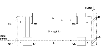
Figure 6: Auxiliary interferometer. M₁ and M₂ are mirrors of g.w. interferometer, M_1r and M_2r are additional mirrors forming the extra resonator, BS and M₀ are beamsplitters and mirrors changing the beam direction.

It is supposed that a small fraction of light is deviated from the main beam to the additional interferometer. As the frequencies of geophysical interest are relatively low, $\sim 10^{-4}Hz$, the relaxation time of the Mach-Zender interferometer should be sufficiently long. If the reflectivity of mirrors $M_{1r}$ and $M_{2r}$ is sufficiently high, a small portion of light can resonate in the cavity for long time, increasing the sensitivity of observation. The added interferometer is capable of measuring the difference of its arm-lengths with high precision. It is interesting to note that this configuration has been actually realised [49], even though the modification is motivated by the struggle with noises rather than by geophysical applications.

The proposed scheme is differential, and therefore it has certain advantages:

- seismic and other common for both arms noises cancel out due to differential character of measurements;

- sudden changes of laser beam position and direction (beam ‘walks’ and ‘jitter’) are not dangerous, as they are common for both arms and cancel out;

- the scheme is universal and can be used at any g.w. interferometer regardless of the actual construction of suspension.

Two other possible modifications, discussed next, are aimed at direct breaking of degeneracy between shifts and tilts in the alignment system. These modificatons do not imply a deviation of light from the main beam of interferometers and, therefore, they are even less likely to compromise the g.w. performance of the instruments.

6.2 Flat mirror behind spherical end mirror.

The desired goal of telling the difference between shifts and tilts of spherical end mirror can be achieved by installation of a flat beamsplitter behind the end mirror. The beamsplitter can be attached to the last stage of the anti-seismic filter. A scheme of this proposal is shown in Fig.7. It is supposed that the beamsplitter (2) intercepts part of light traveling toward the photodetector (3), normally used as an element of the alignment system. The intercepted light is directed through the focusing lens (5) toward the additional photodetector (7). This photodetector should be sensitive to the position of a spot of light focused on the photodetector. For example, the photodetector (7) could consist of two or four pieces, so that a slight movement of the focal spot would produce a differential signal. Since the spherical mirror (1) and the beamsplitter (2) are hanging very close to each other, they participate together in possible shifts of the suspension point and in possible tilts caused by varying local gravity.

Imagine that the mirror (1) and beamsplitter (2) are shifted together in vertical direction (configuration c) in Fig.5). This would lead to no change at the photodetector (7). In contrast, if the mirror (1) and beamsplitter (2) are tilted together (configuration b) in Fig.5), the focal spot will change its position on the photodetector (7) leading to a measurable signal. In this way, the previously indistinguishable configurations b) and c) become distinguishable. If the evaluation (53) of the angular precision remains valid for the proposed scheme, one will be able to extract geophysical information on $\Delta\alpha_{0}$ from this measurement.

Figure 7: A flat mirror (beamsplitter) (2) behind the spherical end mirror (1). A photodetector of the main alignment system is denoted (3), the focusing lens - (5), the last stage of anti-seismic filter - (6), the additional photodetector - (7).

6.3 Additional laser behind the end mirror.

The most natural solution to the formulated problem is, perhaps, the installation of an additional source of light (for some extra details on this proposal, see [50]). Imagine that the additional laser is suspended (possibly, from the same anti-seismic filter) behind the spherical end mirror and shines inside the main cavity, see Fig.8. In order to avoid any mixing of the new light with the already present light in the cavity, the frequency of the auxiliary laser should differ from the frequency of the main laser. However, inside the cavity, the added light satisfies all the usual requirements on mode matching, alignment of the light beam with the optical axis, etc. A possible misalignment of the new beam with the optical axis of the Fabry-Perot resonator will be sensed by the same alignment system and in exactly the same manner as it takes place for the main beam. The only difference is that the detected misalignment of a new beam will be recorded for geophysical studies rather than used for correcting the inclination of the end mirror. One will also need a new photodetector for the output light.

The auxiliary laser and the end mirror are hanging very close to each other, so they react in the same way to shifts of the suspension point or tilts of the plumb line. If the laser itself and the end mirror are both subject to a shift of the suspension point (configuration c) in Fig.5) the alignment of the additional beam with the optical axis of the Fabry-Perot resonator remains intact. The system does not generate an error signal. In contrast, a tilt of the plumb line (configuration b) in Fig.5) will cause a tilt of direction of the incoming beam of the auxiliary laser. This tilt will be detected by the alignment system, thus distinguishing the configurations b) and c). The arising error signal is what we are after. Assuming that the angular sensitivity is still determined by Eq.(53), one will get access to the information on $\Delta\alpha_{0}$. In fact, the installation of an extra laser with properties similar to the ones described above was originally discussed in a different context, with the aim of facilitating the initial tuning of the main interferometer.

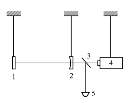
Figure 8: Additional laser behind the end mirror: (1) and (2) - the front and the end mirrors of the main interferometer; (3) - beamsplitter; (4) - additional laser; (5) - additional photodetector.

7 Conclusions

The need for successful functioning of laser-beam detectors of gravitational waves inevitably makes them valuable geophysical instruments. The most immediate application of g.w. detectors is accurate measurement of low-frequency distance variations between the central mirror and the end mirrors. Essentially, the adjustment control system makes the interferometer a low-frequency 3-point meter of deformations. The principal advantage of the existing g.w. detectors in comparison with traditional geophysical techniques is exceptionally long arms of interferometers (a few kilometers in comparison with typical hundred-meter long geophysical interferometers) and high sensitivity of measurements. This advantage leads to a much better strain sensitivity. The extraction of deformational part of the geophysical signal does not imply any hardware modifications, and it can be found in records of the adjustment system right at the level of data analysis.

The alignment system of g.w. laser interferometers on suspended mirrors can potentially provide even more interesting geophysical information - the relative variation of local gravity vectors (plumb lines). This sort of information cannot be obtained from geophysical interferometers which normally use mirrors attached to the ground. It appears, however, that the extraction of this information from the existing g.w. laser interferometers will require certain modest modifications of their optical scheme. Without compromising the astrophysical program of the instruments, these modifications seem to be possible, and we suggested several ways of doing this. Their realization will allow one to use angular measurements in addition to distance measurements. In future advanced g.w. interferometers based on non-spherical mirrors these modifications may be avoided.

The evaluation of interesting geophysical signals and comparison with environmental and instrumental noises shows that the g.w. instruments can reach the most ambitious geophysical goals, such for example as detection of oscillations of the inner core of Earth.

It seems that further progress in this area can be achieved, if a closer collaboration is established between geophysicists and representatives of g.w. community.

References

References

- [1] Thorne K S 1987. In: Three Hundred Years of Gravitation, Eds. S. W. Hawking and W. Israel (Cambridge: CUP) p 330
- [2] Grishchuk L P, Lipunov V M, Postnov K A, Prokhorov M V and Sathyaprakash B S 2001. Usp. Fiz. Nauk, 171 p 3 [Physics-Uspekhi 2001 44 p 1, English transl. ]
- [3] Cutler C and Thorne K S 2002. In: General Relativity and Gravitation, GR16, Eds. N. T. Bishop and S. D. Maharaj (World Scientific) p 72
- [4] Grishchuk L P 2004. In: Astrophysics Update, Ed. J. W. Mason (Springer-Praxis) p 281 (gr-qc/0305051)
- [5] LIGO website http://www.ligo.caltech.edu
- [6] GEO website http://www.geo600.uni-hannover.de
- [7] VIRGO website http://www.virgo.infn.it
- [8] TAMA website http://tamajo.mtk.nao.ac.jp
- [9] Landau L D and Lifshiz E M 1958 Mechanics (Pergamon Press - London)
- [10] Melchior P 1983 The Tides of the Planet Earth (Oxford: Pergamon press)
- [11] Raab F. and Fine M. The effect of Earth tides on LIGO interferometers, LIGO document T970059-01, 2/20/97.
- [12] Bullen K 1978 Earth Density (Moscow: Mir, Russian Transl.)
- [13] Morse P. M. and Feshbach H. Methods of Theoretical Physics, (McGraw-Hill, New York, 1953), Part II, Ch. 11.
- [14] Ness N. F., Harrison J. C. and Slichter L. B. 1961 J. Geophys. Research, 65, p 2
- [15] Benioff H., Press F. and Smith S. 1961 J. Geophys. Research, 65, p 2
- [16] Slichter L B 1961 Proc. Nat. Acad. Sci. USA 47 p 186
- [17] Tanimoto T. and Um J. 1999 J. Geophys. Research. 104, B12, p 723.28
- [18] Jacobs J A 1987 The Earth’s Core (London: International Geophysics Series, Ed. W. L. Donn, Academic press)
- [19] Busse F H 1974 J. Geophys. Research, 79 5 p 753
- [20] Smylie D E 1992 Science 255 p 1678
- [21] Courtier N et al2000 Physics of the Earth and Planetary Interiors 117 p 3
- [22] Kulagin V, Rudenko V., Pasynok S et al2000 (Tokyo:Frontier Science Series ed. S.Kawamura, N.Mio, Univ. Acad. Press) 32 p 343
- [23] Rudenko V and Pasynok S 1997 Frontier Sci. Series (Tokyo: Univ. Acad. Press Inc.) 20 p 63
- [24] Rudenko V 1996 Phys. Lett. A 223 p 421
- [25] Saulson P R 1984 Phys. Rev. D 30 p 732
- [26] Beccaria M et al1998 Class. Quant. Grav. 15 p 3339
- [27] Hughes S A and Thorne K S 1998 Phys. Rev. B 58 p 1202
- [28] Aki K and Richards P 1980 Quantutaitive Seismology. Theory and Methods (San Francisco:ed. W.H.Freeman) 1
- [29] Angew D C 1986 Review of Geophysics 3 p 579
- [30] Rudenko V, Milyukov V, Nesterov V and Ivanov I 1994 Astronomical and Astrophysical Transactions 5 p 93
- [31] Daw E J et al. Long term study of the seismic environment at LIGO, gr-qc/0403046
- [32] Richter B et al. 1995 Marees Terrestres, Bulletin d’Informations, N 122, pp. 1963-1972
- [33] He-Ping Sun 1995 Static deformation and gravity changes at the Earth surface due to atmospheric pressure (Bruxellis: Docteur en Sciences Thesis Observatuire Royal de Belgique)
- [34] Hanada H 1996 Publ. of the Nat. Astron. Observatory of Japan, Tokyo 4 75–78
- [35] Rudenko V, Serdobolski A and Tsubono K 2003 Class. Quant. Grav. 20, p 317
- [36] Grachev A 1998 Izv. Atmosph. Ocean. Phys. 34 p 570
- [37] Gurashvili V, Gusev G, Manukin A, Nikolaev A. 1999 Fizika Zemli (Physics of Earth) 5 p 14
- [38] Landau L D and Lifshitz E M 1959 Fluid Mechanics (Pergamon Press - London)
- [39] Schoemaker D. 2003 Class. Quant. Grav. 20, 10, p S11
- [40] Drever R W P, Hall J L, Kowalski F V et al1983 Appl. Phys. B 31 p 97
- [41] Drever R W P, Hall J L, Kowalski F V et al1983 Appl. Phys. B 32 p 7
- [42] Anderson D 1984 Applied Optics, 23 p 2944
- [43] Sampas N and Anderson D 1990 Applied Optics, 29 p 394
- [44] Kulagin V, Pasynok S, Rudenko V and Serdobolsky A 2001 Large scale laser gravitational interferometer with suspended mirrors for fundamental geodynamics Moscow:Laser Optics’2000, Solid State Lasers, Proc. of SPIE 4350 p 178
- [45] Morrison E, Meers B J, Robertson D I, and Ward H 1994 Applied Optics, 33 50; ibid 33 5037
- [46] Bondarescu M and Thorne K S A new family of light beams and mirror shapes for future LIGO interferometers, gr-qc/0409083
- [47] Drever R 1997 Frontier Sci. Series (Tokyo: Univ. Acad. Press Inc.) 20 p 299
- [48] Drever R and Augst S 2000 Frontier Sci. Series (Tokyo: Univ. Acad. Press Inc.) 32 p 75
- [49] Tsubono K et al2004 Physics Lett. A 327, 1
- [50] Bradaschia C, Braccini S, Giazotto A et al2001 Proc. MG-9, part 2 (World Scientific) p 345