Late-time evolution of charged massive Dirac fields in the Reissner-Nordström black-hole background

Abstract

The late-time evolution of the charged massive Dirac fields in the background of a Reissner-Norström (RN) black hole is studied. It is found that the intermediate late-time behavior is dominated by an inverse power-law decaying tail without any oscillation in which the dumping exponent depends not only on the multiple number of the wave mode but also on the field parameters. It is also found that, at very late times, the oscillatory tail has the decay rate of $t^{-5/6}$ and the oscillation of the tail has the period $2\pi/\mu$ which is modulated by two types of long-term phase shifts.

I introduction

The evolution of field perturbation around a black hole consists roughly of three stages Frolov98 . The first one is an initial wave burst coming directly from the source of perturbation. The second one involves the damped oscillations called the quasinormal modes. And the last one is a power-law tail behavior of the waves at very late time.

The late-time evolution of various field perturbations outside a black hole has important implications for two major aspects of black-hole physics: the no-hair theorem and the mass-inflation scenarioPoisson Burko . Therefore, the decay rate of the various fields has been extensively studied 3 -Ching since Wheeler 1 ; 2 introduced the no-hair theorem. Price 3 studied the massless external perturbations and found that the late-time behavior for a fixed  $r$ is dominated by the factor $t^{-(2l+3)}$. Barack, Ori and Hod considered 7 -9 the late-time tail for the gravitational, electromagnetic, neutrino and scalar fields in the Kerr spacetime. Starobinskii and Novikov Starobinskii analyzed the evolution of a massive scalar field in the RN background and found that there are poles in the complex plane which are closer to the real axis than in the massless case. Hod and Piran 13 pointed out that, if the field mass $\mu$ is small, the oscillatory inverse power-law behavior $\Phi\sim t^{-(l+3/2)}\sin(\mu t)$ dominates as the intermediate late-time tails in the RN background. We Jing1 studied the late-time tail behavior of massive Dirac fields in the Schwarzschild black-hole geometry and found that this asymptotic behavior is dominated by a decaying tail without any oscillation. Koyama and Tomimatsu 14 found that the very late-time tail of the massive scalar field in the Schwarzschild and RN background is approximately given by  $t^{-5/6}\sin(\mu t)$.

Although much attention has been paid to the investigations of the late-time behaviors of the neutral scalar, gravitational and electromagnetic fields in the static and stationary spacetimes, at the moment the study of the late-time tail evolution of the charged massive fields is still an open question. The main purpose of this paper is to study the late-time tail evolution of the charged massive Dirac fields in the RN black-hole background.

II Late-time tail of the charged massive Dirac fields

In the RN spacetime the Dirac equations coupled to a electromagnetic fields Page can be separated by using the Newman-Penrose formalism Newman . After the tedious calculation, we find that the angular equation is the same as in the Schwarzschild black hole Jing1 and the radial equation can be expressed as

$$\frac{d^{2}\Psi_{\pm}}{dr_{*}^{2}}+\left\{\frac{dH_{\pm}}{dr_{*}}-H_{\pm}^{2}+\frac{\Delta}{r^{4}}P_{\pm}\right\}\Psi_{\pm}=0,$$ (1)

with

$$H_{\pm} = \mp\frac{1}{4r^{2}}\frac{d\Delta}{dr}-\frac{\Delta}{r^{3}}\mp\frac{i\mu}{2(\lambda\mp i\mu r)}\frac{\Delta}{r^{2}},$$

$$P_{\pm} = \frac{K^{2}-isK\frac{\Delta}{dr}}{\Delta}+4is\omega r-2iseQ+2s(s+\frac{1}{2})$$

$$+\frac{\mu[\frac{i}{2}(s+\frac{1}{2})\frac{d\Delta}{dr}-K]}{\lambda\mp i\mu r}-\mu^{2}r^{2}-\lambda^{2},$$

where $\Delta=r^{2}-2Mr+Q^{2}$ ($M$ and $Q$ represent the mass and charge of the black hole), $dr_{*}=(r^{2}/\Delta)dr$ and $\Psi_{\pm}=r\Delta^{\pm\frac{1}{4}}(\lambda^{2}+\mu^{2}r^{2})^{-\frac{1}{4}}e^{\pm i\arctan(\frac{\mu r}{\lambda})/2}R_{\pm\frac{1}{2}}$ ($R_{\pm\frac{1}{2}}$ is an usual radial wave function Jing1 ).

Let us assume that both the observer and the initial data are situated far away from the black hole. Then, we can expand Eq. (1) as a power series in $M/r$ and $Q/r$ and obtain (neglecting terms of order $O\left(\left(\omega/r\right)^{2}\right)$ and higher)

$$\left[\frac{d^{2}}{dr^{2}}-\varpi^{2}+\frac{2a\varpi}{r}-\frac{b^{2}-\frac{1}{4}}{r^{2}}\right]\xi_{\pm}=0,$$ (2)

where $\varpi=\sqrt{\mu^{2}-\omega^{2}}$, $a=(M\mu^{2}+eQ\omega)/\varpi-2M\varpi$, $b^{2}=\frac{1}{4}+\lambda^{2}+4M\mu^{2}-Q^{2}(e^{2}+\mu^{2})-2iseQ+(\lambda/\mu+8MeQ+2isM)\omega$ and $\xi_{\pm}=(\Delta/r^{2})^{1/2}\Psi_{\pm}$. We obtain the two basic solutions required to build Green’s function

$$\tilde{\Psi}_{1}=Ae^{-\varpi r}(2\varpi r)^{\frac{1}{2}+b}M(\frac{1}{2}+b-a,1+2b,2\varpi r),$$

$$\tilde{\Psi}_{2}=Be^{-\varpi r}(2\varpi r)^{\frac{1}{2}+b}U(\frac{1}{2}+b-a,1+2b,2\varpi r),$$ (3)

where $A$ and $B$ are normalization constants, $M(\tilde{a},\tilde{b},z)$ and $U(\tilde{a},\tilde{b},z)$ represent the two standard solutions to the confluent hypergeometric equation Abramowitz . $U(\tilde{a},\tilde{b},z)$ is a many-valued function, i.e., there is a cut in $\tilde{\Psi}_{2}$. Hod, Piran and Leaver 13 ; 17 found that the asymptotic massive tail is associated with the existence of a branch cut (in $\tilde{\Psi}_{2}$) placed along the interval $-\mu\leq\omega\leq\mu$ and the branch cut contribution to the Green’s function is

$$G^{C}(r_{*},r_{*}^{\prime};t)=\frac{1}{2\pi}\int_{-\mu}^{\mu}F(\varpi)e^{-i\omega t}d\omega.$$ (4)

with

$$F(\varpi)=$$

$$\frac{\tilde{\Psi}_{1}(r_{*}^{\prime},\varpi e^{i\pi})\tilde{\Psi}_{2}(r_{*},\varpi e^{i\pi})}{W(\varpi e^{i\pi})}-\frac{\tilde{\Psi}_{1}(r_{*}^{\prime},\varpi)\tilde{\Psi}_{2}(r_{*},\varpi)}{W(\varpi)},$$

where $W(\varpi)=W(\tilde{\Psi}_{1},\tilde{\Psi}_{2})=\tilde{\Psi}_{1}\tilde{\Psi}_{2,x}-\tilde{\Psi}_{2}\tilde{\Psi}_{1,x}$ is the Wronskian. We obtain, with the help of Eq. (13.1.22) of Ref. Abramowitz , that $W(\varpi e^{i\pi})=-W(\varpi)=AB\frac{\Gamma(2b)}{\Gamma(1/2+b-a)}4b\varpi$. For simplicity we assume that the initial data has a considerable support only for $r$ values which are smaller than the observer’s location. This, of course, does not change the late-time behavior. Noting that when $t$ is large, the term $e^{-i\omega t}$ oscillates rapidly. This leads to a mutual cancellation between the positive and the negative parts of the integrand, so that the effective contribution to the integral arises from $|\omega|=O(\mu-\frac{1}{t})$ or equivalently $\varpi=O(\sqrt{\mu/t})$ 13 . Using Eqs. (13.1.32), (13.1.33) and (13.1.34) of Ref. Abramowitz , we find that $F(\varpi)$ is given by

$$F(\varpi) = \frac{r_{*}^{\frac{1}{2}-b}r_{*}^{\prime\frac{1}{2}+b}e^{-\varpi(r_{*}+r_{*}^{\prime})}}{2b}[M(\frac{1}{2}+b+a,1+2b,2\varpi r_{*}^{\prime})M(\frac{1}{2}-b+a,1-2b,2\varpi r_{*})-M(\frac{1}{2}+b-a,1+2b,2\varpi r_{*}^{\prime})$$ (5)

$$\times M(\frac{1}{2}-b-a,1-2b,2\varpi r_{*})]-\frac{\Gamma(-2b)\Gamma(\frac{1}{2}+b-a)}{\Gamma(2b)\Gamma(\frac{1}{2}-b-a)}\frac{(4\varpi^{2}r_{*}r_{*}^{\prime})^{\frac{1}{2}+b}e^{-\varpi(r_{*}+r_{*}^{\prime})}}{4\varpi b}[M(\frac{1}{2}+b-a,1+2b,2\varpi r_{*}^{\prime})$$

$$\times M(\frac{1}{2}+b-a,1+2b,2\varpi r_{*})+e^{(1+2b)i\pi}M(\frac{1}{2}+b+a,1+2b,2\varpi r_{*}^{\prime})M(\frac{1}{2}+b+a,1+2b,2\varpi r_{*})].$$

We first focus our attention on the intermediate asymptotic behavior of the charged massive Dirac fields. That is the tail in the range $M\ll r\ll t\ll M/(M\mu)^{2}$. In this time scale, we find that the frequency range $\varpi=O(\sqrt{\mu/t})$, which gives the dominant contribution to the integral, implies $a\ll 1$. Equation (2) shows that $a$ originates from the $1/r$ term which describes the effect of backscattering off the spacetime curvature. That is to say, the backscattering off the spacetime curvature from the asymptotically far regions is negligible for the case $a\ll 1$. Then, using the fact that $M(\tilde{a},\tilde{b},z)\approx 1$ as $z\rightarrow 0$, we have

$$F(\varpi) = \frac{\pi}{sin(\pi b)}\frac{1+e^{(1+2b)i\pi}}{2^{1+2b}b^{2}}\frac{\varpi^{2b}}{\Gamma(b)^{2}}(r_{*}r_{*}^{\prime})^{1/2+b}.$$ (6)

Substituting Eq. (6) into the Eq. (4), we find

$$G^{C}(r_{*},r_{*}^{\prime};t)=$$

$$\int_{-\mu}^{\mu}\frac{(1+e^{(1+2b)i\pi})(r_{*}r_{*}^{\prime})^{\frac{1}{2}+b}}{2^{2b+1}b^{2}\Gamma(b)^{2}sin(\pi b)}(\mu^{2}-\omega^{2})^{b}e^{-i\omega t}d\omega.$$ (7)

Unfortunately, the integral (II) can not be evaluated analytically since the parameter $b$ depends on $\omega$. However, we can work out the integral numerically and the corresponding results are presented in Figs. 1-3. Figure 1 describes $\ln|G^{C}(r_{*},r_{*}^{\prime};t)|$ versus $t$ for different $eQ$, which shows that the dumping exponent depends on $seQ$, i.e., the product of the spin weight of the Dirac fields and the charges of the black hole and Dirac fields, and $seQ<0$ speeds up the decay of the perturbation but $seQ>0$ slows it down. Figure 2 illustrates $\ln|G^{C}(r_{*},r_{*}^{\prime};t)|$ versus $t$ for different $\lambda$ with $s=\pm 1/2$, $\mu=0.01$ and $eQ=0.01$, which indicates that the dumping exponent depends on the multiple number of the wave mode, and the larger the magnitude of the multiple number, the more quickly the perturbation decays. Figure 3 gives $\ln|G^{C}(r_{*},r_{*}^{\prime};t)|$ versus $t$ for different mass $\mu$ of the Dirac fields, which shows that the dumping exponent depends on the mass of the Dirac fields, and the smaller the mass $\mu$, the faster the perturbation decays.

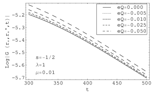
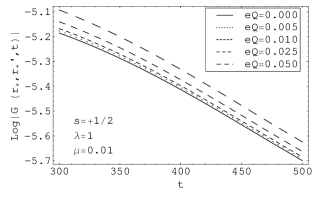
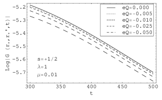
Figure 1: Graphs of $\ln|G^{C}(r_{*},r_{*}^{\prime};t)|$ versus $t$ for different $seQ$. These figures show that the dumping exponent depends on the product of the spin weight and the charges of the black hole and Dirac fields, and $seQ<0$ speeds up the perturbation decay but $seQ>0$ slows it down.

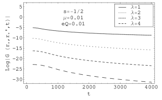
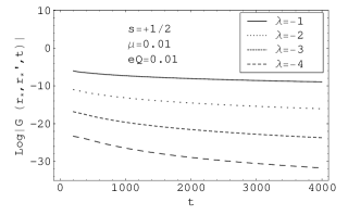
Figure 2: Graphs of $\ln|G^{C}(r_{*},r_{*}^{\prime};t)|$ versus $t$ for different $\lambda$ with $s=\pm 1/2$, $\mu=0.01$ and $eQ=0.01$, showing that the dumping exponent depends on the multiple number of the wave mode, and the larger the magnitude of multiple number, the more quickly the perturbation decays.

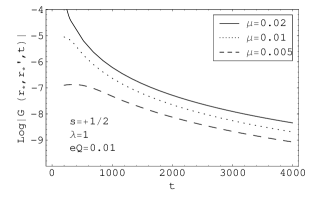
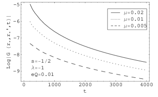
Figure 3: Graphs of $\ln|G^{C}(r_{*},r_{*}^{\prime};t)|$ versus $t$ for different mass $\mu$. The result obtain from these figures is that the dumping exponent depends on the mass of the Dirac fields, and the smaller the mass $\mu$, the faster the perturbation decays.

In the above discussion we have used the approximation of  $a\ll 1$, which only holds when  $\mu t\ll 1/(\mu M)^{2}$. Therefore, the power-law tail found earlier is not the final one, and a change to a different pattern of decay is expected when $a$ is not negligibly small. Here we examine the asymptotic tail behavior at very late times such that $\mu t\gg 1/(\mu M)^{2}$. This asymptotic tail behavior is caused by a resonance backscattering due to spacetime curvature 14 . In this case, we have $a\simeq(M\mu^{2}+eQ\mu)/\varpi\gg 1$, namely, the backscattering off the spacetime curvature in asymptotically far regions is important. Using Eq. (13.5.13) of Ref. Abramowitz and Eq. (5), we obtain

$$F(\omega)\simeq\frac{\Gamma(1+2b)\Gamma(1-2b)r_{*}^{\prime}r_{*}}{2b}$$

$$[J_{2b}(\sqrt{\alpha r_{*}^{\prime}})J_{-2b}(\sqrt{\alpha r_{*}})-I_{2b}(\sqrt{\alpha r_{*}^{\prime}})I_{-2b}(\sqrt{\alpha r_{*}})]$$

$$+\frac{\Gamma(1+2b)^{2}\Gamma(-2b)r_{*}^{\prime}r_{*}}{2b\Gamma(2b)}\frac{\Gamma(\frac{1}{2}+b-a)}{2b\Gamma(\frac{1}{2}-b-a)}a^{-2b}$$

$$[J_{2b}(\sqrt{\alpha r_{*}^{\prime}})J_{2b}(\sqrt{\alpha r_{*}})+I_{2b}(\sqrt{\alpha r_{*}^{\prime}})I_{2b}(\sqrt{\alpha r_{*}})],$$ (8)

where $\alpha=8(M\mu^{2}+eQ\mu)$, and $I_{\pm(2b)}$ is the modified Bessel function.

We can study late-time behavior for the first term of Eq. (II) using numerical method. The result is presented by Fig. 4 which shows that asymptotically late-time tail arising from the first term is still $\sim t^{-1}$ although the factor $\Gamma(1+2b)\Gamma(1-2b)/2b$ is not a constant.

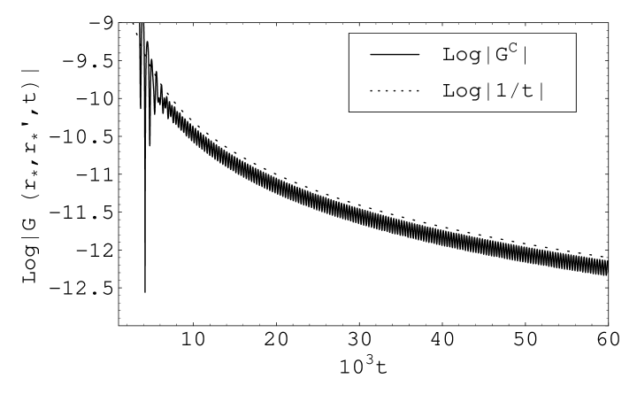
Figure 4: Graphs of $\ln|G^{C}(r_{*},r_{*}^{\prime};t)|$ versus $t$ with $M=100$, $\mu=0.01$, $s=-1/2$, $\lambda=1$, $Q=0.1M$ and $e=0.002$ for the first term (solid line). The dashed line is $\sim\log\left|1/t\right|$.

Now let us to find the behavior of the second term. Because of $\Gamma(1+2b)\Gamma(1-2b)/2b=-\Gamma(1+2b)^{2}\Gamma(-2b)/(2b\Gamma(2b))$ and the factor $\Gamma(1+2b)\Gamma(1-2b)/2b$ almost dose not affect the asymptotical behavior of the first term, we can define

$$C = \frac{\Gamma(1+2b)^{2}\Gamma(-2b)r_{*}^{\prime}r_{*}}{2b\Gamma(2b)}[J_{2b}(\sqrt{\alpha r_{*}^{\prime}})J_{2b}(\sqrt{\alpha r_{*}})$$

$$+I_{2b}(\sqrt{\alpha r_{*}^{\prime}})I_{2b}(\sqrt{\alpha r_{*}}),$$

which approximates to a constant. Then, in the limit $a\gg 1$, the contribution of the second term to the Green’s function can be expressed as

$$G^{C}(r_{*},r_{*}^{\prime};t)\sim\frac{C}{2\pi}\int_{-\mu}^{\mu}e^{i(2\pi a-\omega t)}e^{i\phi}d\omega,$$ (9)

where the phase $\phi$ is determined by $e^{i\phi}=\frac{1+(-1)^{2b}e^{-2i\pi a}}{1+(-1)^{2b}e^{2i\pi a}},$ and it remains in the range $0\leq\phi\leq 2\pi$, even if $a$ becomes very large. We use saddle-point integration to evaluate Eq. (9) and find

$$G^{C}(r_{*},r_{*}^{\prime};t)\sim\frac{C\mu}{2\sqrt{3}}\left(2\pi\right)^{\frac{5}{6}}(M\mu+2eQ)^{\frac{1}{3}}(\mu t)^{-\frac{5}{6}}$$

$$sin\{\mu t-[2\pi(M\mu+2eQ)]^{\frac{2}{3}}(\mu t)^{\frac{1}{3}}-\phi(\omega_{0})-\frac{\pi}{4}\},$$ (10)

which is the asymptotic behavior of the Green’s function at very late times. Eq. (10) shows that the decay rate of the asymptotic tail is $t^{-5/6}$ and the oscillation of the tail has the period $2\pi/\mu$ which is modulated by two types of long-term phase shifts, a monotonously increasing phase shift $[2\pi(M\mu+2eQ)]^{\frac{2}{3}}(\mu t)^{\frac{1}{3}}$ and a period phase shift $\phi(\omega_{0})$.

To confirm the analytical prediction, we present the numerical result of the second term in Fig. 5 and find that the decay rate of the asymptotic tail is still $t^{-5/6}$.

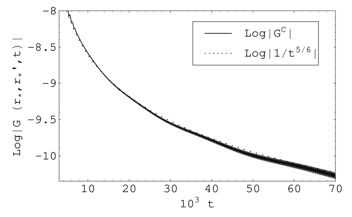
Figure 5: Graphs of $\ln|G^{C}(r_{*},r_{*}^{\prime};t)|$ versus $t$ with $M=100$, $\mu=0.01$, $s=-1/2$, $\lambda=1$, $Q=0.1M$ and $e=0.002$ for the second term (solid line). The dashed line is $\sim\log\left|t^{-5/6}\right|$.

III summary

The intermediate late-time tail and the asymptotic tail behavior of the charged massive Dirac fields in the background of the RN black hole are studied. The results of the intermediate late-time tail are presented by figures because we can not obtain analytically Green’s function $G^{C}(r_{*},r_{*}^{\prime};t)$ because the parameter $b$ in the integrand of the Green’s function depends on the integral variable $\omega$. We learn from the figures that the intermediate late-time behavior is dominated by an inverse power-law decaying tail without any oscillation, which is different from the oscillatory decaying tails of the scalar fields. It is interesting to note that the dumping exponent depends not only on the multiple number of the wave mode but also on the mass of the Dirac fields and the product $seQ$. We also find that the decay rate of the asymptotically late-time tail is $t^{-5/6}$ and the oscillation of the tail has the period $2\pi/\mu$ which is modulated by two types of long-term phase shifts.

References

• (1) V. P. Frolov, and I. D. Novikov, Black hole physics: basic concepts and new developments (Kluwer Academic, Dordrecht, 1998).
• (2) E. Poisson and W. Israel, Phys. Rev. D 41, 1796 (1990).
• (3) L. M. Burko, Phys. Rev. Lett. 79, 4958 (1997); ibid. 90, 121101 (2003); ibid. 90, 249902 (2003).
• (4) R. H. Price, Phys. Rev. D 5, 2419 (1972).
• (5) L. Barack and A. Ori, Phys. Rev. Lett. 82, 4388 (1999).
• (6) S. Hod, Phys. Rev. Lett. 84, 10 (2000).
• (7) S. Hod, Phys. Rev. D 58, 104022 (1998).
• (8) A. A. Starobinskii and I. D. Novikov (unpublished).
• (9) S. Hod and T. Piran, Phys. Rev. D 58, 044018 (1998).
• (10) Jiliang Jing, Phys. Rev. D 70, 065004 (2004).
• (11) H. Koyama and A. Tomimatsu, Phys. Rev. D 63, 064032 (2001); ibid. D 64, 044014 (2001).
• (12) S. Hod and T. Piran, Phys. Rev. D 58, 024017 (1998).
• (13) S. Hod and T. Piran, Phys. Rev. D 58, 024019 (1998).
• (14) J. Karkowski, Z. Swierczynski, and E. Malec, gr-qc/0303101.
• (15) Qiyuan Pan and Jiliang Jing, Chin. Phys. Lett. 21(10), 1873 (2004).
• (16) N. Andersson, Phys. Rev. D 55, 468 (1997).
• (17) L. M. Burko and A. Ori, Phys. Rev. D 56, 7820 (1997).
• (18) L. M. Burko and G. Khanna, Phys. Rev. D 70, 044018 (2004).
• (19) E. W. Allen, E. Buckmiller, L. M. Burko, and R. H. Price, Phys. Rev. D 70, 044038 (2004).
• (20) C. Gundlach, R. H. Price, and J. Pullin, Phys. Rev. D 49, 890 (1994).
• (21) M. A. Scheel, A. L. Erickcek, L. M. Burko, L. E. Kidder, H. P. Pfeiffer, and S. A. Teukolsky, Phys. Rev. D 69, 104006 (2004).
• (22) E. S. C. Ching, P. T. Leung, W. M. Suen, and K. Young, Phys. Rev. D 52, 2118 (1995).
• (23) R. Ruffini and J. A. Wheeler, Phys. Today 24(1), 30 (1971).
• (24) C. W. Misner, K. S. Thorne, and J. A. Wheeler, Gravitation (Freeman, San Francisco, 1973).
• (25) D. N. Page, Phys. Rev. D 14, 1509 (1976).
• (26) E. Newman and R. Penrose, J. Math. Phys. (N. Y.) 3, 566 (1962).
• (27) M. Abramowitz and I. A. Stegun,  $Handbook\ \ of\ \ Mathematical\ \ Functions$ (Dover, New York, 1970).
• (28) E. W. Leaver, Phys. Rev. D 34, 384 (1986).